Effect of winding edge currents

Abstract

We discuss persistent currents for particles with internal degrees of freedom. The currents arise because of winding properties essential for the chaotic motion of the particles in a confined geometry. The currents do not change the particle concentrations or thermodynamics, similar to the skipping orbits in a magnetic field.

1 Introduction

Windings of random walk trajectories are of considerable interest in various fields of condensed matter physics, from polymers and DNA to superconductors and Bose-Einstein condensates (see e.g. [1, 2, 3] and references therein). In this paper, we consider the influence of winding on the internal degrees of freedom of particles dynamics.

Note that winding dependent degrees of freedom are not exotic. The most obvious of these is, of course, the spin, which is of particular interest in view of the recent spintronic surge of activity. Because of the spin-orbit interaction, the spin is directly related to the winding of particle trajectories. Accordingly, our analysis is intimately related to the so-called spin Hall effect in electron transport [4, 5, 6, 7, 8, 9, 10] as well as to other types of spin transport, like, for example, photon (light) propagation in disordered media (since photons also have non-zero spin).

Other degrees of freedom, both classical and quantum, can also be winding dependent, as e.g. geometric phases (the Berry phase). Thus, the results of the present work are applicable not only to spin transport but also to any situation that can be reduced to random trajectories in a confined geometry with the dependence of certain characteristics on winding properties.

The paper is organized as follows. Section 2 presents the concept of winding and the corresponding terminology. Section 3 deals with the spin degree of freedom as directly dependent on a winding angle. Section 4 contains numerical simulations in the case of diffusion in a rectangular 2d domain with periodic boundary conditions in the longitudinal direction and hard walls in the transverse direction. Section 5 proposes a simple theoretical model of classical random walks with so-called “soft walls”, where the geometric constraints are described by an external confining potential in the transverse direction. Section 6 contains a brief discussion of the results.

2 Winding of curved trajectories

Let us introduce the winding angle $\boldsymbol{\theta}$ as the vector sum of all the turnings of a particle trajectory $\boldsymbol{x}(t)$. The angle is called the total curvature in the literature (see e.g. [11, 12]). It is given by the integral of the differential curvature over a natural parameter (the local time of the trajectory). The differential curvature $\boldsymbol{\kappa}$ of the trajectory is defined as

$$\boldsymbol{\kappa}=|\boldsymbol{\dot{x}}|^{-3}\boldsymbol{\dot{x}}\times\boldsymbol{\ddot{x}},$$

where the symbol “$\,\dot{\;}\,$”  denotes differentiation with respect to $t$ and the symbol $\times$ denotes the vector product. Correspondingly, $\boldsymbol{\theta}$ has the form [13]

$$\boldsymbol{\theta}=\int^{t}_{0}\boldsymbol{\kappa}(t)|\boldsymbol{\dot{x}}(t)|dt=\int_{0}^{t}\frac{\boldsymbol{v}\times\boldsymbol{\dot{v}}}{v^{2}}dt,\ \boldsymbol{v}\equiv\boldsymbol{\dot{x}}.$$ (1)

Note that the total curvature of a closed planar trajectory, equal to the ”winding number” or ”turning number” multiplied by $2\pi$, is a homotopy invariant.

It is worth mentioning that the term “winding angle” is also used in polymer physics (see e.g. [3]) where, however, it rather refers to

$$\boldsymbol{\vartheta}=\int^{t}_{0}\frac{\boldsymbol{x}\times\boldsymbol{\dot{x}}}{x^{2}}dt.$$

Thus, $\boldsymbol{\vartheta}$ is the winding angle of the radius vector of the trajectory in configuration space, whereas $\boldsymbol{\theta}$ yields an analogous quantity but in velocity space.

The distribution of $\boldsymbol{\vartheta}$’s for Brownian trajectories has been studied for a long time (see e.g. [2, 3, 14]), while that of $\boldsymbol{\theta}$’s has not been analyzed so far. On the other hand, it seems that $\boldsymbol{\theta}$ is a more appropriate quantity for certain problems, for example those including spin (spin Hall effect, etc), as we will argue below.

We consider for simplicity the 2d case. Generalizations to 3d and tensors are fairly simple, but the resulting formulas are more involved and less intuitive. In the planar case the winding angle vector $\boldsymbol{\theta}$ is normal to the plane, hence it suffices to consider $\theta$, the unique non-zero component of $\boldsymbol{\theta}$.

The transport of the winding angle is described by the average current density

$$\boldsymbol{j}(\boldsymbol{x})=\langle\theta\boldsymbol{v}\delta(\boldsymbol{x}-\boldsymbol{x}(t))\rangle,$$ (2)

where the symbol $\langle\dots\rangle$ denotes averaging over a set of Brownian trajectories, or, in the discrete case, of random walks.

In the case of an infinite plane (or a plane with periodic boundary conditions) and of equilibrium, the particle density does not depend on the coordinates and the average $\langle\theta\rangle$ vanishes identically as well as the average of the winding current density (2). If, however, a confined planar geometry is considered, then $\langle\theta\rangle$ will still be vanishing but, as we will show below, this will not be the case for the winding current, because of the geometrical constraints. Namely, due to the mere existence of boundaries, there will exist trajectories whose contribution to the winding will not be canceled by that of other trajectories. As a result, there will necessarily appear an anti-parallel edge current with $\theta>0$ and $\theta<0$ and $\boldsymbol{j}$ will not identically vanish anymore. These surviving edge currents can be viewed as analogs of spin edge currents in the spin Hall effect [15].

3 Spin-orbit interaction and winding

Before considering the winding currents, it is useful to discuss briefly an important example of spin-orbit interaction where the spin degree of freedom depends on the winding angle $\theta$.

It seems known that in electronic transport in the presence of charged impurities the electron spin depends on the winding of their trajectories. This dependence manifests itself, for instance, as the so called skew scattering in the “extrinsic” spin Hall effect [7, 8]. However, in the literature on the subject, the concept of trajectory winding is mostly implicit.

Recall that in electronic transport impurities interact with electrons and thus the scattering angle, hence the deviation of the electron trajectory from a ballistic straight line, depends, in relativistic theory, on the spin. More generally, it is known that if, for any reason (not necessarily related to electrons scattering on charged impurities) the trajectory of a relativistic particle is not a straight line, the curving of the trajectory changes the spin degree of freedom of the particle. This purely kinematic relativistic effect is due to the successive non-parallel Lorentz transformations (boosts) that lead to the so-called Wigner rotation of the spin, or the Thomas-Wigner precession.

The variation of the precession angle of a classical rotating moment resulting from an infinitesimal turning of the velocity has been obtained by Thomas [16, 17, 18]

$$d\boldsymbol{\varphi}\approx\frac{1}{2c^{2}}\boldsymbol{v}\times d\boldsymbol{v}\ ,$$ (3)

where $\boldsymbol{\varphi}$ is a vector of the precession angle, $\boldsymbol{v}$ is the velocity, $d\boldsymbol{v}$ its variation, and $c$ is the speed of light.

Eq. (3) gives the leading relativistic approximation for the precession angle. It is worth mentioning that the exact relativistic expression is still a matter of controversy (see the recent articles [19, 20, 21]). Note also that the Dirac equation allows for a more precise study of this effect. However the classical result (3) of Thomas is sufficiently accurate to describe well the spin-orbit splitting in atoms [22]. It has played an important role in the genesis of the quantum theory of radiation (see e.g [18]).

Comparing (1) and (3), we find a simple relation between the moment precession angle and the winding angle of the trajectory

$$d\boldsymbol{\varphi}\approx\frac{v^{2}}{c^{2}}d\boldsymbol{\theta}\ ,$$ (4)

where $d\boldsymbol{\theta}$ is the trajectory turning angle. Note that, in many cases, the precession angle during the observation time is essentially equal to the winding angle multiplied by a small parameter $v^{2}/c^{2}$ (e.g. the case of fermions at temperatures below Fermi temperature, or any particles in the case of elastic scattering).

Let us now argue that the spatial curvature of a trajectory is equivalent to the action of a magnetic field on a spin degree of freedom. Indeed, it is known that an homogeneous magnetic field in the rest frame of a classical spin results in its Larmor precession [23]

$$\dot{\boldsymbol{s}}=\frac{ge}{2mc}\boldsymbol{s}\times\boldsymbol{H}\ ,$$

where $\boldsymbol{s}$ is the spin in angular momentum units, $\boldsymbol{H}$ is the magnetic field, $g$ is the gyro-magnetic factor, and $m$ is the mass. Thus, an effective magnetic field with a Larmor frequency equal to the frequency $\dot{\boldsymbol{\varphi}}$ of Thomas-Wigner precession ($\dot{\boldsymbol{s}}=\boldsymbol{s}\times\dot{\boldsymbol{\varphi}}$) has the form

$$\boldsymbol{H}_{eff}=\frac{2mc}{ge}\dot{\boldsymbol{\varphi}}\approx\frac{m}{egc}\boldsymbol{v}\times\boldsymbol{\dot{v}}\equiv\frac{2mv^{2}}{egc}\boldsymbol{\dot{\theta}}\ .$$ (5)

The spin-field interaction energy is then

$$E=\frac{ge}{2mc}\boldsymbol{s}\cdot\boldsymbol{H_{eff}}=\frac{\boldsymbol{s}\cdot(\boldsymbol{v}\times\boldsymbol{\dot{v}})}{2c^{2}}\equiv\frac{v^{2}}{c^{2}}\ \boldsymbol{s}\cdot\dot{\boldsymbol{\theta}}\ .$$

Hence, the direction and the magnitude of the effective magnetic field are intimately related to the winding angle.

Returning to random walks of electrons in solids (which can result from electrons scattering on charged impurities, see e.g. [24]), we note that in this case it follows from (5) that the effective magnetic field of the Lorentz transformation of the impurity electric field can be included in the Wigner-Thomas precession and vice versa, thus forming a complete spin-orbit interaction.

We also note that, leaving aside electrons in solids, the above discussion can refer in general to the diffusion of any particles with non-zero spin or magnetic moment in disordered media, for example spin 1 photons whose motion in a medium with random refractive index can be described as a diffusion process [24, 25, 26]), as well as in foams, metamaterials, dense plasma, etc…(see e.g. [27] and references therein).

4 Numerical simulations

Let us now turn to numerical simulations which do support the existence of winding edge currents. We consider the strip of width $L_{1}$ along the horizontal axis and of length $L_{2}$ along the vertical axis on a planar square lattice of period 1. In the longitudinal direction periodic boundary conditions are imposed at $x_{2}=0,L_{2}$. In the transverse direction reflecting (hard) walls enclose the strip in a finite width $x_{1}=0,L_{1}$.

We consider $N_{p}$ independent particles whose trajectories are random walks on the lattice. The diffusion time step $\tau$ is assumed to be unity and random hoppings are allowed only to the nearest neighbor sites. Let

$$\boldsymbol{x}(k,i)=\sum_{m=0}^{k}\Delta\boldsymbol{x}(m,i)$$

and $\theta(k,i)$ be respectively the position and the winding angle of the $i$th particle after $k$ jumps. It is clear that each next turn (left or right) increases or decreases $\theta(k,i)$ by $\pi/2$. We assume, for the sake of definiteness, that a backward scattering does not change the winding angle of the trajectory.

The time averaged winding current $\boldsymbol{j}(\boldsymbol{x})$ at a point $\boldsymbol{x}$ of the lattice is after $N$ steps (i.e. during the observation time $t=N$)

$$\boldsymbol{j}(\boldsymbol{x})=\frac{1}{N}\sum_{i}\sum_{k=0}^{N}\theta(k,i)\boldsymbol{v}(k,i)\delta_{\boldsymbol{x},\boldsymbol{x}(k,i)}\ ,$$ (6)

where $\delta_{\boldsymbol{x},\boldsymbol{x^{\prime}}}$ is the Kronecker delta.

We analyzed a wide range of parameters $L_{1}$, $L_{2}$, $N$, and $N_{p}$. Typical results are shown in Fig.1 for $N_{p}=4000$, $N=500000$, and strip sizes $L_{1}=L_{2}=100$. To display the 2d vector field $\boldsymbol{j}$, we use a 2d palette as in Fig.1(b). The palette center corresponds to zero vector field and its vertical and horizontal edges correspond to the range of the components $j_{1}$ and $j_{2}$ of $\boldsymbol{j}(\boldsymbol{x})$, respectively. The palette is divided in four sectors of different colors with a radial variation of the color intensity. This allows to distinguish the approximate direction and magnitude of the current.

The numerical simulations for $\boldsymbol{j}(\boldsymbol{x})$ are shown in Fig.1(a).

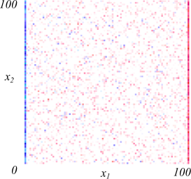
(a) $\boldsymbol{j}(\boldsymbol{x})$

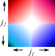
(b) 2d palette

(c) $L_{2}^{-1}\int^{L_{2}}_{0}dx_{2}j_{2}(\boldsymbol{x_{2}})$

Figure 1: 1(a) – the winding current $\boldsymbol{j}$. 1(b) – the 2d palette. 1(c) – the winding current component $j_{2}$ averaged over $x_{2}$ as a function of $x_{1}$.

In the bulk of the sample only small-scale fluctuations of the winding current can be seen. However, things differ strongly from the bulk in the narrow neighborhoods of the walls: winding currents do exist along the edges. They materialize as almost continuous and narrow lines on the left and right edges of the sample (blue and red, according to the direction). The non vanishing longitudinal component of the winding current, averaged over $x_{2}$, is displayed in Fig.1(c). It is concentrated within one lattice site from the edges and directed downward near the left edge and upward near the right edge.

Fig.2 displays the absolute value of the current density $|\boldsymbol{j}(\boldsymbol{x})|$ and how it concentrates on the edges with an increase of the simulation time $N$.

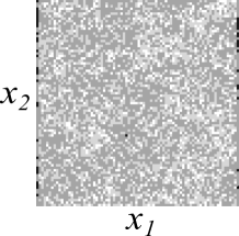
(a) $N=5000$

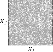
(b) $N=10000$

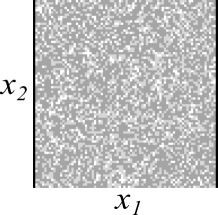
(c) $N=100000$

Figure 2: The modulus $|\boldsymbol{j}(\boldsymbol{x})|$ for different values of $N$ with $N_{p}=3000$. The darker the dot, the bigger the modulus of $\boldsymbol{j}$.

Since the system is in equilibrium, i.e., external fields are absent and the particles are distributed uniformly, winding currents can only originate from the confining boundaries and the chaotic kinetic energy of the random walk trajectories. Thus, these currents are by nature persistent.

5 A simple solvable model

Let us consider a simple model where the effect of winding currents is explicit. It consists of planar continuous Brownian trajectories described by an Ornstein-Uhlenbeck process in a potential $U$ applied along the $x_{1}$ axis and infinitely growing as $|x_{1}|\to\infty$. The potential plays the role of the “soft walls” confining the Brownian particles, and thereby encodes the geometric constraints. As in the previous section, periodic boundary conditions at $x_{2}=0,L_{2}$ are assumed in the longitudinal direction.

The stochastic (Langevin) equations of motion are

$$\dot{x_{i}} = v_{i}$$ (7)

$$\dot{v_{i}} = -\frac{1}{m}\frac{\partial U}{\partial x_{i}}-\beta v_{i}+\xi_{i}$$

where $\boldsymbol{x}=(x_{1},x_{2})$ is the coordinate of the particle, $\boldsymbol{v}=(v_{1},v_{2})$ is its velocity, $m$ is the mass of the particle, $\beta$ is the viscosity and $\boldsymbol{\xi}=(\xi_{1},\xi_{2})$ is the random force assumed to be the Gaussian white noise, i.e.

$$\langle\xi_{i}(t)\rangle=0,\quad\langle\xi_{i}(t^{\prime})\xi_{j}(t^{\prime\prime})\rangle=D\delta_{ij}\delta(t^{\prime}-t^{\prime\prime}).$$ (8)

Since we are interested in the winding of trajectories of the above random process, we consider the joint probability density of the coordinate, velocity and winding angle $\theta$

$$p(t,\boldsymbol{x},\boldsymbol{v},\theta)=\langle\delta(\boldsymbol{x}-\boldsymbol{x}(t))\delta(\boldsymbol{v}-\boldsymbol{v}(t))\delta(\theta-\theta(t))\rangle\ .$$ (9)

The $\theta$ integration of (9) yields the density $P(t,\boldsymbol{x},\boldsymbol{v})$ satisfying the usual Kramers equation [28] (Fokker-Planck equation with external potential)

$$\frac{\partial}{\partial t}P=-v_{i}\frac{\partial}{\partial x_{i}}P+\frac{1}{m}\frac{\partial U}{\partial x_{i}}\frac{\partial}{\partial v_{i}}P+\beta\frac{\partial}{\partial v_{i}}v_{i}P+\frac{D}{2}\frac{\partial^{2}}{\partial v_{i}^{2}}P\ .$$ (10)

where $D$ is defined in (8) and the standard summation convention over repeated indices is understood.

It is easy to check that the probability density $P$ in (10) converges as $t\to\infty$ to a stationary Maxwell-Boltzmann distribution in $x_{1}$ and $\boldsymbol{v}$ with a $L_{2}^{-1}$ normalization factor in the longitudinal direction $x_{2}$ (see (15)). Note that one could also use reflecting boundary conditions or a weak confining potential in this direction.

The Fokker-Planck equation for $p(t,\boldsymbol{x},\boldsymbol{v},\theta)$ can be obtained as follows. Let us denote

$$\mathfrak{\Delta}=\delta(\boldsymbol{x}-\boldsymbol{x}(t))\delta(\boldsymbol{v}-\boldsymbol{v}(t))\delta(\theta-\theta(t)),$$

then $p=\langle\mathfrak{\Delta}\rangle$ and

$$\frac{\partial}{\partial t}p=-\frac{\partial}{\partial x_{i}}\langle\dot{x_{i}}\mathfrak{\Delta}\rangle-\frac{\partial}{\partial v_{i}}\langle\dot{v_{i}}\mathfrak{\Delta}\rangle-\frac{\partial}{\partial\theta}\langle\frac{\epsilon_{ij}v_{i}\dot{v_{j}}}{v^{2}}\mathfrak{\Delta}\rangle\ .$$

Then eq. (7) implies

$$\frac{\partial}{\partial t}p+v_{i}\frac{\partial}{\partial x_{i}}p=\frac{\partial}{\partial v_{i}}\Big{(}\frac{1}{m}\frac{\partial U}{\partial x_{i}}+\beta v_{i}\Big{)}p+\\ \frac{1}{mv^{2}}\epsilon_{ij}v_{i}\frac{\partial U}{\partial x_{j}}\frac{\partial}{\partial\theta}p-\frac{1}{v^{2}}\Big{[}\frac{\partial}{\partial v_{i}}\delta_{ij}+\epsilon_{ij}v_{i}\frac{\partial}{\partial\theta}\Big{]}\langle\xi_{j}\mathfrak{\Delta}\rangle\ .$$ (11)

To deal with the correlation functions $\langle\xi_{j}\mathfrak{\Delta}\rangle$, we use the Furutsu-Novikov formula (see e.g. [29], Chapter 10 and [30], Chapter 5) valid for any functional $R_{t}[\xi]$ of the $\delta$-correlated Gaussian random functions $\xi_{1}$ and $\xi_{2}$

$$\langle\xi_{j}(t)R_{t}[\xi]\rangle=\frac{D}{2}\Big{\langle}\frac{\delta}{\delta\xi_{j}(t)}R_{t}[\xi]\Big{\rangle}\ .$$

We obtain after integration by parts

$$\langle\xi_{j}(t)\mathfrak{\Delta}\rangle=-\frac{D}{2}\frac{\partial}{\partial x_{k}}\Big{\langle}\frac{\delta x_{k}(t)}{\delta\xi_{j}(t)}\mathfrak{\Delta}\Big{\rangle}-\frac{D}{2}\frac{\partial}{\partial v_{k}}\Big{\langle}\frac{\delta v_{k}(t)}{\delta\xi_{j}(t)}\mathfrak{\Delta}\Big{\rangle}-\frac{D}{2}\frac{\partial}{\partial\theta}\Big{\langle}\frac{\delta\theta(t)}{\delta\xi_{j}(t)}\mathfrak{\Delta}\Big{\rangle}\ .$$ (12)

To find the variational derivatives of $x_{k}$ and $v_{k}$ with respect to $\xi_{j}$, we apply the operation $\delta/\delta\xi(\tau)$ to the integrated Langevin equations, then use the principle of causality and take the limit $\tau\rightarrow t$. This yields

$$\frac{\delta x_{k}(t)}{\delta\xi_{j}(\tau)}=\int\limits_{\tau}^{t}\frac{\delta v_{k}(t_{1})}{\delta\xi_{j}(\tau)}dt_{1}\xrightarrow{\tau\rightarrow t}0\ ,$$

and

$$\frac{\delta v_{k}(t)}{\delta\xi_{j}(\tau)}=\delta_{kj}-\beta\int\limits_{\tau}^{t}\frac{\delta v_{k}(t_{1})}{\delta\xi_{j}(\tau)}dt_{1}-\frac{1}{m}\int\limits_{\tau}^{t}\frac{\partial^{2}U}{\partial x_{k}\partial x_{i}}(\boldsymbol{x}(t_{1}))\frac{\delta x_{i}(t_{1})}{\delta\xi_{j}(\tau)}dt_{1}\xrightarrow{\tau\rightarrow t}\delta_{kj}\ .$$

The variational derivative of $\theta$ in (12) is calculated using (1)

$$\frac{\delta\theta(t)}{\delta\xi_{j}(\tau)}=\frac{\delta}{\delta\xi_{j}(\tau)}\epsilon_{ik}\int\limits_{0}^{t}dt_{1}\frac{v_{i}(t_{1})\Big{(}-\beta v_{k}(t_{1})-\displaystyle{\frac{1}{m}\frac{\partial U}{\partial x_{k}}(\boldsymbol{x}(t_{1}))}+\xi_{k}(t_{1})\Big{)}}{v^{2}(t_{1})}\$$

and finally

$$\frac{\delta\theta(t)}{\delta\xi_{j}(\tau)}=\epsilon_{ik}\delta_{jk}\frac{v_{i}(\tau)}{v^{2}(\tau)}-\frac{\epsilon_{ik}}{m}\int\limits_{\tau}^{t}dt_{1}\{...\}\xrightarrow{\tau\rightarrow t}-\epsilon_{ji}\frac{v_{i}(\tau)}{v^{2}(\tau)}\ .$$

Thus, the correlation functions $\langle\xi_{j}\mathfrak{\Delta}\rangle$ are expressed via the partial derivatives of $p$

$$\langle\xi_{j}(t)\mathfrak{\Delta}\rangle=-\frac{D}{2}\frac{\partial}{\partial v_{j}}p+\frac{D}{2}\epsilon_{ji}\frac{v_{i}}{v^{2}}\frac{\partial}{\partial\theta}p\ .$$

We assume for the sake simplicity that the diffusion coefficient $D$ does not depend on the velocity and we take into account the relation $\epsilon_{ij}\epsilon_{jk}=-\delta_{ik}$. We obtain the Fokker-Plank equation

$$\frac{\partial}{\partial t}p + v_{i}\frac{\partial}{\partial x_{i}}p=\frac{\partial}{\partial v_{i}}\Big{(}\frac{1}{m}\frac{\partial U}{\partial x_{i}}+\beta v_{i}\Big{)}p+\frac{D}{2}\frac{\partial^{2}}{\partial v_{i}^{2}}p$$

$$+ \frac{1}{m}\epsilon_{ij}\frac{v_{i}}{v^{2}}\frac{\partial U}{\partial x_{j}}\frac{\partial}{\partial\theta}p+D\epsilon_{ij}\frac{v_{i}}{v^{2}}\frac{\partial^{2}}{\partial v_{j}\partial\theta}p+\frac{D}{2v^{2}}\frac{\partial^{2}}{\partial\theta^{2}}p\ .$$

In the case at hand where the potential $U$ depends only on the transverse coordinate $x_{1}$ (modeling the soft walls of a deep valley) the Fokker-Planck equation becomes

$$\frac{\partial}{\partial t}p + v_{i}\frac{\partial}{\partial x_{i}}p-\frac{\partial}{\partial v_{1}}\frac{1}{m}U^{\prime}(x_{1})p-\beta\frac{\partial}{\partial v_{i}}v_{i}p-\frac{D}{2}\frac{\partial^{2}}{\partial v_{i}^{2}}p$$

$$=-\frac{1}{m}\frac{v_{2}}{v^{2}}U^{\prime}(x_{1})\frac{\partial}{\partial\theta}p+D\frac{v_{1}}{v^{2}}\frac{\partial^{2}}{\partial v_{2}\partial\theta}p-D\frac{v_{2}}{v^{2}}\frac{\partial^{2}}{\partial v_{1}\partial\theta}p+\frac{D}{2}\frac{1}{v^{2}}\frac{\partial^{2}}{\partial\theta^{2}}p\ .$$

Eq. (5) differs from the Kramers equation by the terms on the right-hand side. The physical meanings of the first and fourth terms are the most interesting. It is already clear here and will be even more clear below that the former is the current in the $x_{2}$ direction and the latter is responsible for the diffusive spreading of $\theta$.

We also note that after integration over $\theta$ (5) coincides with the Kramers equation (10).

Eq. (5) allows us to study the transfer of arbitrary $\theta$-dependent quantities as well as non-equilibrium situations corresponding to arbitrary initial conditions. In the particular case of the winding current (2), which is linear in $\theta$, the steady-state current can be found without actually solving the equation.

Indeed, it is clear that the transverse component $j_{1}$ of the mean current density $\boldsymbol{j}$ vanishes. To find the average longitudinal component $j_{2}$ let us multiply (5) by $\theta v_{2}$ and integrate over $\boldsymbol{v}$ and $\theta$. We obtain after integration by parts

$$\frac{\partial j_{2}}{\partial t}=-\beta j_{2}+\frac{1}{m}U^{\prime}(x_{1})\int d\boldsymbol{v}\frac{v_{2}^{2}}{v^{2}}P(t,\boldsymbol{x},\boldsymbol{v})\ .$$ (14)

The probability density $P(t,\boldsymbol{x},\boldsymbol{v})$ approaches for large time the stationary distribution

$$P_{st}=\frac{\beta}{\pi DZL_{2}}\exp\left(-\frac{\beta}{D}v^{2}-\frac{2\beta}{mD}U(x_{1})\right),$$ (15)

where

$$Z=\int_{-\infty}^{+\infty}e^{-\frac{2\beta}{mD}U(x_{1})}dx_{1}$$

is a normalization constant. It follows then from (14) and (15) that for $t>>\beta^{-1}$ the current $j_{2}$ relaxes to its stationary form

$$j_{2}(x_{1})=\frac{1}{2m\beta L_{2}}U^{\prime}(x_{1})P_{B}(x_{1})$$ (16)

where

$$P_{B}(x_{1})\equiv\frac{1}{Z}e^{-\frac{2\beta}{mD}U(x_{1})}$$

is the steady state (Boltzmann) probability distribution in the transverse direction.

We obtain finally for the local average density of winding current per unit length in the longitudinal direction

$$J_{2}(x_{1})=\frac{n}{2m\beta}U^{\prime}(x_{1})P_{B}(x_{1})\ ,$$ (17)

where $n=N_{p}/L_{2}$ is the number of particles per unit length in the longitudinal direction.

The average winding current density (17) is proportional to the gradient of the potential and to the local density of diffusing particles, which is determined by the temperature and the height of the potential at a given point $x_{1}$. One can easily see that the currents are antiparallel on opposite walls. The gradient of the potential and the Boltzmann distribution also determine the currents width. Particular examples of currents profiles are shown in Figure 3 for an harmonic potential $U(x_{1})=x_{1}^{2}$ and a trapezoidal potential $U(x_{1})=\eta(-1-x_{1})|x_{1}+1|+\eta(x_{1}-1)|x_{1}-1|$, where $\eta(x)$ is the Heaviside step function [ $\eta(x)=1$ for $x>0$, and $\eta(x)=0$ for $x\leq 0$ ].

   

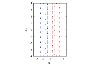
(a) $U(x_{1})=x_{1}^{2}$

   

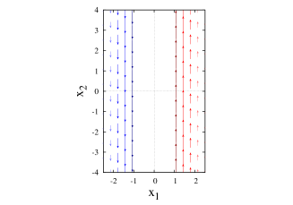
(b) $U(x_{1})=\eta(-1-x_{1})|x_{1}+1|+\eta(x_{1}-1)|x_{1}-1|$

Figure 3: The winding current density in the harmonic and trapezoidal potentials and the profile $J_{2}(x_{1})$ in arbitrary dimensionless units. On the profile charts, the left y-axis is $J_{2}$ and the right y-axis is $U$.

Note that formula (16) can be interpreted (up to a small relativistic factor) as describing the diffusion of magnetic moments in an effective magnetic field $\boldsymbol{H}\propto[\boldsymbol{v}\times\nabla U]$, thereby corresponding to the setting of the spin Hall effect in the potential $U$, as already mentioned above. We recall that in our approach there is no interaction, and no magnetic (or any other type) moments. We are only dealing with distributions of trajectories winding, hence the above effect can be viewed as purely dynamical (“winding Hall effect”).

Assume finally without loss of generality that $U(0)=0$. Then the spatial average of $J_{2}$ in (17) over $(0,\infty)$ (or $(-\infty,0)$) is

$$\int_{0}^{\infty}J_{2}(x_{1})dx_{1}=\int_{-\infty}^{0}J_{2}(x_{1})dx_{1}=\frac{nD}{4Z\beta^{2}}.$$ (18)

This can be viewed as a manifestation of the weak dependence of our results on the concrete form of the confining potential (considering that $n/Z$ is the effective planar density of particles).

6 Conclusion

We demonstrated that random walks or continuous Brownian motions in a confined planar geometry generate dissipationless persistent currents of degrees of freedom associated with the winding of their trajectories. This is a purely edge effect where the currents are formed in a close neighborhood of the boundaries. In the case of the “soft walls”, where the geometric confinement is provided by an infinitely growing transverse potential, the channel width of the current is determined by the gradient of the potential and the thermal energy of the particles. In the case of reflecting boundaries (“hard-walls”), the channel width is just a single diffusion step, according to the numerical simulations.

In the microscopic world, the spin and geometric phase are examples of degrees of freedom which depend on the winding. Note that it is commonly believed that in the spin Hall effect the dissipationless edge currents arise in the conditions of the quantum “intrinsic” regime, where dissipation and chaos are absent because of quantization. Since, however, the above “extrinsic” spin Hall effect corresponds to an ordinary diffusion, thus to a sufficiently high dissipation, one would think that persistent spin currents should not occur. However, as we have shown, this is not the case simply because of the chaotic kinetic energy of the random trajectories of the particles.

Similar effects may occur in purely mechanical systems where relativistic or quantum phenomena are absent. For example, the torque of a compass arrow in a moving car is also a degree of freedom which ”feels” the curvature of the car trajectory. Thus, the effect studied here can be of interest beyond the scope of phenomena associated with the spin Hall effect.

In the case of the Ornstein-Uhlenbeck model with soft walls we have obtained an analytical expression for the persistent current of the winding via the Boltzmann distribution in an arbitrary transverse confining potential. The kinetic equation takes into account the winding of particles and, in principle, allows to explore the joint probability distributions in the single-particle phase space of the degrees of freedom with an arbitrary dependence on the winding.

7 Acknowledgement

This work was supported by the Ukrainian Branch of the French-Russian Poncelet Laboratory and the Grant 23/12-N of the National Academy of sciences of Ukraine. Stéphane Ouvry would like to thank the B. Verkin Institute for Low temperatures and Engineering for hospitality during the initial stages of the work.

LIST OF FIFGURES

Figure 1. (a) – the winding current $\boldsymbol{j}$. (b) – the 2d palette. (c) – the winding current component $j_{2}$ averaged over $x_{2}$ as a function of $x_{1}$.

Figure 2. The modulus $|\boldsymbol{j}(\boldsymbol{x})|$ for different values of $N$ with $N_{p}=3000$. The darker the dot, the bigger the modulus of $\boldsymbol{j}$.

Figure 3. The winding current density in the harmonic and trapezoidal potentials and the profile $J_{2}(x_{1})$ in arbitrary dimensionless units. On the profile charts, the left y-axis is $J_{2}$ and the right y-axis is $U$.

References

- [1] D. M. Ceperley, Rev. Mod. Phys. 67, 279 (1995).
- [2] J. Desbois, and S. Ouvry, J. Stat. Mech. P05024 (2011) and P05005 (2012).
- [3] A. Grosberg, and H Frisch, J. Phys. A: Math. Gen. 36 (2003) 8955.
- [4] M. I. Dyakonov and V. I. Perel, Sov. Phys. JETP Lett. 13, 467469 (1971).
- [5] J. E. Hirsch, Phys. Rev. Lett. 83, 18341837 (1999).
- [6] S. Zhang, Phys. Rev. Lett. 85, 393396 (2000).
- [7] H.-A. Engel, B. I. Halperin, and E. I. Rashba, Phys. Rev. Lett. 95, 166605 (2005).
- [8] W.-K. Tse and S. Das Sarma, Phys. Rev. Lett. 96, 056601 (2006).
- [9] N. P. Stern, D. W. Steuerman, S. Mack, A. C. Gossard, and D. D. Awschalom, Nature Physics 4, 843 (2008)
- [10] T. Jungwirth, J. Wunderlich, and K. Olejnik, Nature Materials 11, 382390 (2012).
- [11] J. W. Milnor, The Annals of Mathematics, 52(2), 248 (1950).
- [12] John M. Sullivan, in Discrete Differential Geometry, Oberwolfach Seminars 38, (Birkhäuser, 2008) pp. 137-161; arXiv:math/0606007 (2007).
- [13] W. Kühnel, Differential Geometry: Curves - Surfaces - Manifolds, (Amer Mathematical Society, 2006).
- [14] F. Spitzer, Trans. Amer. Math. Soc. 87 (1958) 187
- [15] Y. Zhou and F.-C. Zhang, Nature Physics 8, 448449 (2012).
- [16] L. H. Thomas, Nature 117, 514 (1926).
- [17] J. D. Jackson, Classical Electrodynamics, (Wiley Inc., 1998) p. 808.
- [18] S.-I. Tomonaga, and T. Oka, The Story of Spin, (University of Chicago Press, 1997)
- [19] G. B. Malykin, Physics-Uspekhi 49, 837 (2006).
- [20] V. I. Ritus, Physics-Uspekhi 50, 95 (2007).
- [21] Y. Y. Zanimonskiy and Yu. P. Stepanovsky, Kharkov Uiversity Bulletin 899, 23 (2010).
- [22] J. Kessler, Polarized Electrons, (Springer, 1985) p. 299.
- [23] V. Bargmann, L. Michel, and V. L. Telegdi, Phys.Rev.Lett. 2, 435 (1959).
- [24] E. Akkermans, and G. Montambaux, Mesoscopic Physics of Electrons and Photons (Cambridge University Press, 2007).
- [25] J. R. Lorenzo Principles Of Diffuse Light Propagation, (World Scientific, 2012).
- [26] P. Sheng Introduction to Wave Scattering, Localization and Mesoscopic Phenomena, (Springer, 2006).
- [27] M. Storzer, P. Gross, C. M. Aegerter, and G. Maret, Phys. Rev. Lett. 96, 063904 (2006).
- [28] N. G. Van Kampen, Stochastic Processes in Physics and Chemistry, (Elsevier, 2007) p. 464.
- [29] I. M. Lifshits, S. A. Gredeskul, and L. A. Pastur, Introduction to the Theory of Disordered Systems (Wiley Inc., 1988) p. 357.
- [30] V. I. Klyatskin, Dynamics of Stochastic Systems, Elsevier, Amsterdam, 2005, p.212