On asymptotics of ICA estimators and their performance indices

Abstract

Independent component analysis (ICA) has become a popular multivariate analysis and signal processing technique with diverse applications. This paper is targeted at discussing theoretical large sample properties of ICA unmixing matrix functionals. We provide a formal definition of unmixing matrix functional and consider two popular estimators in detail: the family based on two scatter matrices with the independence property (e.g., FOBI estimator) and the family of deflation-based fastICA estimators. The limiting behavior of the corresponding estimates is discussed and the asymptotic normality of the deflation-based fastICA estimate is proven under general assumptions. Furthermore, properties of several performance indices commonly used for comparison of different unmixing matrix estimates are discussed and a new performance index is proposed. The proposed index fullfills three desirable features which promote its use in practice and distinguish it from others. Namely, the index possesses an easy interpretation, is fast to compute and its asymptotic properties can be inferred from asymptotics of the unmixing matrix estimate. We illustrate the derived asymptotical results and the use of the proposed index with a small simulation study.

Keywords: Independent Component Analysis; Performance Indices; FastICA; FOBI; Asymptotic Normality.

1 Introduction

In the independent component (IC) model we assume that the components of the observed $p$-variate random vector $x=(x_{1},...,x_{p})^{T}$ are linear combinations of the components of a latent $p$-vector $z=(z_{1},...,z_{p})^{T}$ such that $z_{1},...,z_{p}$ are mutually independent. Then

$$x=\Omega z$$ (1)

where $\Omega$ is a full-rank $p\times p$ mixing matrix. The model is semiparametric as we do not make any assumptions on the marginal distributions of $z_{1},...,z_{p}$. In order to be able to identify a mixing matrix one has to assume that at most one of the components $z_{1},...,z_{p}$ is normally distributed, Hyvärinen et al. (2001). Still after this assumption, the parameter matrix $\Omega$ is not uniquely defined: Let $\mathcal{C}$ be the set of $p\times p$ matrices with exactly one non-zero element in each row and in each column. If $C\in\mathcal{C}$ then also $z^{*}=Cz$ has independent components and the model can be rewritten as $x=\Omega^{*}z^{*}$ where $\Omega^{*}=\Omega C^{-1}$.

There are several possible, but not always satisfactory, solutions to this identifiability problem. One then fixes $C$ by fixing either $z^{*}=Cz$ or $\Omega^{*}=\Omega C^{-1}$ in some way. First, the random vector $z^{*}=Cz$ can be fixed by requiring, for example, that the components of $z^{*}$ satisfy (i) $Var(z^{*}_{i})=1$, $i=1,...,p$, (ii) $\beta_{1}(z^{*}_{i})>0$, $i=1,...,p$, and (iii) $\beta_{2}(z^{*}_{1})>...>\beta_{2}(z^{*}_{p})$ where $\beta_{1}$ and $\beta_{2}$ are classical moment-based skewness and kurtosis measures, respectively. The above idea was extended in Ilmonen et al. (2010a); Nordhausen et al. (2011a) by fixing the random vector $Cz$ using two different location vectors and two different scatter matrices with the so called independence property. In these approaches, some indeterminacy still remains for random vectors with identical or symmetrical marginal distributions, for example. Second, the transformation matrix $\Omega^{*}=\Omega C^{-1}$ can be fixed by requiring, for example, that $||\Omega C^{-1}-I_{p}||$ is minimized. Ilmonen and Paindaveine (2011) used a unique representation $\Omega C^{-1}$ such that all the diagonal elements of $\Omega C^{-1}$ are one. In this paper we accept the ambiguity in the model (1), and try to define our concepts and analysis tools so that they are independent of the model specification, that is, of the specific choices of $z$ and $\Omega$.

In the independent component analysis (ICA) the aim is to find an estimate for an unmixing matrix $\Gamma$ such that $\Gamma x$ has independent components. Again, if $\Gamma$ is a mixing matrix then so is $C\Gamma$ for all possible matrices $C\in\mathcal{C}$. Thus $\Gamma=\Omega^{-1}$ in the model (1) is just one possible unmixing matrix and the ICA problem reduces to estimating an unmixing matrix $\Omega^{-1}$ only up to the order, signs and scales of the rows of $\Omega^{-1}$. In the signal processing and computer science communities ICA procedures are usually seen as algorithms rather than estimates with their statistical properties. The most popular algorithms, if formulated with random variables, then often proceed as follows.

1. In the model (1), one can assume without loss of generality that $Cov(z)=I_{p}$. Then, after whitening, we get the random vector

   $$y=Cov(x)^{-1/2}(x-E(x))=V(z-E(z))$$

   with some orthogonal matrix $V$.

2. Using $y$, find a orthogonal matrix $U=(u_{1},...,u_{p})^{T}$ with the rows $u_{i}$, $i=1,...,p$, chosen to maximize (or minimize) a criterion function, say $\sum_{i=1}^{p}|E[G(u_{i}^{T}y)]|$. The optimization may be conducted one by one or simultaneously. The function $G$ (measure of non-gaussianity, negentropy, kurtosis measure, log-likelihood function, etc.) is chosen so that the solution is $U=V^{T}$ up to possible sign changes and permutations of the rows.

3. The final ICA solution is then $\Gamma=UCov(x)^{-1/2}$.

The fastICA algorithms described in Hyvärinen and Oja (1997) for example works in this way. The rows of $U$ are then found either one after another (deflation-based fastICA) or simultaneously (symmetric fastICA). The sample versions are naturally obtained by replacing the expectations by corresponding sample averages. For detailed descriptions of the fastICA procedures and several other estimates and algorithms, see Cichocki and Amari (2006) and Hyvärinen et al. (2001). For other type of estimates, see Chen and Bickel (2005) and Chen and Bickel (2006).

Due to the vast amount of different ICA estimates and algorithms, asymptotic as well as finite sample criteria are needed for their comparisons. While results on asymptotic statistical properties (convergence, asymptotic normality, etc.) are usually missing in the literature, several finite-sample performance indices have been proposed for the comparisons in simulation studies. Let $\hat{\Gamma}$ be an unmixing matrix estimate based on the random sample $X=(x_{1},...,x_{n})^{T}$ from the distribution in model (1). First, one can compare the “true” sources $z_{i}$ (which are of course known in the simulations) and the estimated sources $\hat{z_{i}}=\hat{\Gamma}x_{i}$, $i=1,...,n$. Second, one can measure the closeness of the “true” unmixing matrix $\Omega^{-1}$ (used in the simulations) and the estimated unmixing matrix $\hat{\Gamma}$. In both cases the problem is that $\hat{\Gamma}$ is typically not an estimate for $\Omega^{-1}$. However, for any reasonable estimate $\hat{\Gamma}$, either (i) there exists a $C\in\mathcal{C}$ such that $\hat{\Gamma}$ is a consistent estimate of $\Omega C^{-1}$, or (ii) there exists a (possibly unknown or unspecified) matrix $\hat{C}\in\mathcal{C}$ such that $\hat{C}\hat{\Gamma}$ is a consistent estimate of $\Omega^{-1}$. Therefore, for a good estimate, the gain matrix $\hat{G}=\hat{\Gamma}\Omega$ tends to be close to some matrix $C\in\mathcal{C}$. In this paper we discuss performance indices that are based on the use of $\hat{G}=\hat{\Gamma}\Omega$. A new index is proposed that finds the shortest distance (using Frobenius norm) between the identity matrix and the set of matrices equivalent to the gain matrix $\hat{\Gamma}\Omega$.

We organize the paper as follows. First, in Section 2, we give a formal (mathematical) definition of the IC functional which is independent of the model formulation. We consider two families of IC functionals, (i) the family based on two scatter matrices with independence property, and (ii) the family of deflation-based fastICA functionals. We review limiting behavior of the corresponding estimates and we prove the asymptotic normality of the deflation-based fastICA under certain general assumptions. Previous attempts to prove the asymptotic normality of the deflation-based fastICA that have been presented in the literature contain severe faults. In Section 3 we consider the use of the gain matrix in the comparison of different IC estimates. Several approaches are discussed in detail. In Section 4 a new index for the comparison is introduced. The computation of the new index is shown to be straightforward and easy. We also consider the limiting behavior of the index as the sample size approaches infinity; the asymptotic properties of the index are in a natural way determined by the asymptotic properties of the estimate $\hat{\Gamma}$. The finite sample vs. asymptotic behavior of the index for several different ICA estimates with known asymptotics is illustrated in a small simulation study. Most proofs of the theorems are placed in the Appendix.

2 IC functionals

In this section we give a formal (mathematical) definition of an independent component (IC) functional. The definition is independent of the model formulation, that is, of the choice of $\Omega$ and $z$. As an example we consider the family of IC functionals based on two scatter matrices with independence property, and the family of deflation-based fastICA functionals.

2.1 Formal definition

Let $\mathcal{G}$ be the set of all full-rank $p\times p$ matrices. Then naturally all unmixing matrices $\Gamma\in\mathcal{G}$. Let $P$ denote a permutation matrix (obtained from $I_{p}$ by permuting its rows or columns), $J$ a sign-change matrix (a diagonal matrix with diagonal elements $\pm 1$), $D$ a rescaling matrix (a diagonal matrix with positive diagonal elements). For the definition of an IC functional we need the subset

$$\mathcal{C} = \left\{C\in\mathcal{G}:C=PJD\ \ \mbox{for some $P$, $J$, and $D$}\right\}.$$

If $C\in\mathcal{C}$, each row and each column of $C$ has exactly one nonzero element. Then $\mathcal{C}$ gives a group of affine transformations (with respect to matrix multiplication) as it satisfies (i) if $C_{1},C_{2}\in\mathcal{C}$ then $C_{1}C_{2}\in\mathcal{C}$, (ii) $I_{p}\in\mathcal{C}$, (iii) if $C\in\mathcal{C}$ then there exists $C^{-1}\in\mathcal{C}$ such that $CC^{-1}=C^{-1}C=I_{p}$. The group is not commutative (Abelian) as $C_{1}C_{2}=C_{2}C_{1}$ may not be true.

We say that two matrices $\Gamma_{1}$ and $\Gamma_{2}$ in $\mathcal{G}$ are equivalent if $\Gamma_{1}=C\Gamma_{2}$ for some $C\in\mathcal{C}$. We then write $\Gamma_{1}\sim\Gamma_{2}$ and give the following definition.

Definition 2.1.

Let $F_{x}$ denote the cdf of $x$ The functional $\Gamma(F_{x})\in\mathcal{G}$ is an IC functional in the IC model (1) if (i) $\Gamma(F_{x})\Omega\sim I_{p}$ and if (ii) it is affine equivariant in the sense that $\Gamma(F_{Ax})=\Gamma(F_{x})A^{-1}$ for all nonsingular $p\times p$ matrices $A$.

Remark 2.1.

The first condition says that $\Gamma(F_{x})$ and $\Omega^{-1}$ are equivalent matrices and that there exists $C=C(F_{x},\Omega)\in\mathcal{C}$ such that the “adjusted” IC functional $C\Gamma(F_{x})=\Omega^{-1}$. Note that, if the second condition (ii) is replaced by a weaker condition (iii) $\Gamma(F_{Ax})\sim\Gamma(F_{x})A^{-1}$ for all nonsingular matrices $A$, then one can often find a new functional

$$\Gamma^{*}(F_{x})=C(F_{x})\Gamma(F_{x})$$

with $C(F_{x})\in\mathcal{C}$ satisfying condition (ii). If the fourth moments exist, functional $C=C(F_{x})$ may be defined by requiring, for example, that $Var((\Gamma^{*}x)_{i})=1$, $i=1,...,p$, $\beta_{1}((\Gamma^{*}x)_{i})>0$, $i=1,...,p$, and $\beta_{2}((\Gamma^{*}x)_{1})>...>\beta_{2}((\Gamma^{*}x)_{p})$ where $\beta_{1}$ and $\beta_{2}$ are classical moment-based skewness and kurtosis measures, respectively. Then $\Gamma^{*}(F_{Ax})=\Gamma^{*}(F_{x})A^{-1}$ for all nonsingular $p\times p$ matrices $A$. Other criteria for constructing $C(F_{x})$ can be easily found.

Remark 2.2.

In practice, the IC functional is often seen rather as a set of vectors $\{\gamma_{1},...,\gamma_{p}\}$ than as a matrix $\Gamma=(\gamma_{1},...,\gamma_{p})^{T}$. If $P_{i}=||\gamma_{i}||^{-2}\gamma_{i}\gamma_{i}^{T}$ is the projection matrix to the subspace spanned by $\gamma_{i}$, $i=1,...,p$, then the functional can also be defined as a set of projection matrices $\{P_{1},...,P_{p}\}$.

Note that, for an IC functional $\Gamma$ in model (1) $\Gamma(F_{x})\Omega C\sim I_{p}$ for all $C\in C$. Therefore the definition of the IC functional does not depend on the specific formulation of the model (the choices of $\Omega$ and $z$). Also, $\Gamma(F_{x})x=\Gamma(F_{z})z$ where $\Gamma(F_{z})$ is in $\mathcal{C}$. If we choose $z^{*}=\Gamma(F_{z})z$ and $\Omega^{*}=\Omega\Gamma(F_{z})^{-1}$, then $\Gamma(F_{x})\Omega^{*}=I_{p}$. This formulation of the model is then most natural (canonical) for functional $\Gamma(F_{x})$.

2.2 Functionals based on two scatter matrices

A scatter functional $S(F_{x})$ is a $p\times p$ -matrix-valued functional which is positive definite and affine equivariant in the sense that

$$S(F_{Ax+b})=AS(F_{x})A^{T}$$

for all nonsingular $p\times p$ matrices $A$ and for all $p$-vectors $b$. A scatter functional $S$ is said to possess the independence property if $S(F_{x})$ is a diagonal matrix for all $x$ with independent components. Naturally, the usual covariance matrix

$$S_{1}(F_{x})=E\left((x-E(x))(x-E(x))^{T}\right)$$

is a scatter matrix with the independence property. Another scatter matrix with the independence property is the matrix based on fourth moments, namely,

$$S_{2}(F_{x})=\frac{1}{p+2}E\left((x-E(x))(x-E(x))^{T}S_{1}(F_{x})^{-1}(x-E(x))(x-E(x))^{T}\right).$$

For any scatter matrix $S(F_{x})$, its symmetrized version

$$S_{sym}(F_{x})=S(F_{x_{1}-x_{2}}),$$

where $x_{1}$ and $x_{2}$ are independent copies of $x$, has the independence property, Oja et al (2006); Tyler et al. (2009). For symmetrized M-estimators and S-estimators, see Roelandt et al. (2009); Sirkiä et al. (2007).

The IC functional $\Gamma(F_{x})$ based on the scatter matrix functionals $S_{1}(F_{x})$ and $S_{2}(F_{x})$ is defined as a solution of the equations

$$\Gamma S_{1}\Gamma^{T}=I_{p}\ \ \mbox{and}\ \ \Gamma S_{2}\Gamma^{T}=\Lambda$$

where $\Lambda=\Lambda(F_{x})$ is a diagonal matrix with diagonal elements $\lambda_{1}\geq...\geq\lambda_{p}>0$. One of the first solutions for the ICA problem, the FOBI functional, Cardoso (1989), is obtained if the scatter functionals $S_{1}$ and $S_{2}$ are the scatter matrices based on the second and fourth moments, respectively. The use of two scatter matrices in ICA has been studied in Nordhausen et al. (2008); Oja et al (2006) (real data) and in Ollila et al. (2008b); Ilmonen (2012) (complex data).

Assume now (wlog) that $\Omega=I_{p}$ and that $S_{1}(F_{x})=I_{p}$ and $S_{2}(F_{x})=\Lambda$ where $\lambda_{1}>...>\lambda_{p}>0$. Assume also that both $S_{1}$ and $S_{2}$ have the independence property. Write $\hat{S_{1}}=S_{1}(F_{n})$ and $\hat{S_{2}}=S_{2}(F_{n})$ (values of the functionals at the empirical cdf $F_{n}$). We then have the following result, Ilmonen et al. (2010a).

Theorem 2.1.

Assume that

$$\sqrt{n}(\hat{S}_{1}-I_{p})=O_{p}(1)\ \ \mbox{and}\ \ \sqrt{n}(\hat{S}_{2}-\Lambda)=O_{p}(1),$$

with $\lambda_{1}>...>\lambda_{p}>0$, and the estimates $\hat{\Gamma}$ and $\hat{\Lambda}$ are given by

$$\hat{\Gamma}\hat{S}_{1}\hat{\Gamma}^{T}=I_{p}\ \ \mbox{and}\ \ \hat{\Gamma}\hat{S}_{2}\hat{\Gamma}^{T}=\hat{\Lambda}.$$

Then, there exists a sequence of estimators such that $\hat{\Gamma}\to_{P}I_{p}$,

$$\sqrt{n}\mbox{diag}(\hat{\Gamma}-I_{p}) = -\frac{1}{2}\sqrt{n}\mbox{diag}(\hat{S}_{1}-I_{p})+o_{p}(1)\ \ \mbox{and}$$

$$\sqrt{n}\ \mathrm{off}(\hat{\Gamma}-I_{p}) = \sqrt{n}\ H\odot\left((\hat{S}_{2}-\Lambda)-(\hat{S}_{1}-I_{p})\Lambda\right)+o_{p}(1),$$

where $H$ is a $p\times p$ matrix with elements

$$H_{ij}=0,\ \mbox{if}\ i=j,\ \ \mbox{and}\ \ H_{ij}=(\lambda_{i}-\lambda_{j})^{-1},\ \mbox{if}\ i\neq j.$$

Above $\mathrm{off}(\Gamma)=\Gamma-\mathrm{diag}(\Gamma),$ where $\mathrm{diag}(\Gamma)$ is a diagonal matrix with the same diagonal elements as $\Gamma$, and $\odot$ denotes the Hadamard (entrywise) product. Ilmonen et al. (2010a) considered the limiting distribution of the FOBI estimate (with limiting covariance matrix) in more detail. It is interesting to note that the asymptotic behavior of the diagonal elements of $\hat{\Gamma}$ does not depend on $\hat{S}_{2}$ at all.

Approaches such as JADE, Cardoso and Souloumiac (1993), or the matrix-pencil approach, Yeredor (2009), (approximately) jointly diagonalize two or more data matrices (not necessarily scatter matrices). The asymptotic properties of these estimates are typically however still unknown.

2.3 Deflation-based FastICA functionals

Our second example on families of IC functionals is given by the deflation-based fastICA algorithm. FastICA is one of the most popular and widespread ICA algorithms. Detailed examination of fastICA functionals are provided for example in Hyvärinen and Oja (1997) and Ollila (2010). In Ollila (2010), the asymptotic covariance structure of the row vectors of deflation-based fastICA estimate $\hat{\Gamma}$ is given in closed form. No rigorous proof of the asymptotic normality of the fastICA estimate has been presented in the literature so far; see for example Shimizu et al. (2006). In this section we discuss the conditions needed for the asymptotic normality of the deflation-based fastICA estimate.

Assume that $x=\Omega z$ as in model (1) with finite first and second moments $E(x)=\mu$ and $Cov(x)=\Sigma$. In this approach the first row of $\Gamma$ is obtained when a criterion function $|E(G(\gamma^{T}(x-\mu)))|$ is maximized under the constraint $\gamma^{T}\Sigma\gamma=1$. If we wish to find more than one source then, after finding $\gamma_{1},...,\gamma_{k-1}$, the $k$th source maximizes $|E(G(\gamma^{T}(x-\mu)))|$ under the constraint

$$\gamma_{k}^{T}\Sigma\gamma_{k}=1\ \ \mbox{and}\ \ \gamma_{j}^{T}\Sigma\gamma_{k}=0,\ \ j=1,...,k-1.$$

If $G$ satisfies the condition

$$|E(G(\alpha_{1}z_{1}+\alpha_{2}z_{2}))|\leq\max(|E(G(z_{1}))|,|E(G(z_{2}))|)$$

for all independent $z_{1}$ and $z_{2}$ such that $E(z_{1})=E(z_{2})=0$ and $E(z_{1}^{2})=E(z_{2}^{2})=1$ and for all $\alpha_{1}$ and $\alpha_{2}$ such that $\alpha_{1}^{2}+\alpha_{2}^{2}=1$, then the independent components are found using the above strategy. It is easy to check that the condition is true for the classical kurtosis measure $G(z)=z^{4}-3$, for example (Bugrien, 2005).

Write $T(F)$ for the mean vector (functional) and $S(F)$ for the covariance matrix (functional). The $k$th fastICA functional $\gamma_{k}(F)$ then optimizes the Lagrangian function

$$|E[G(\gamma_{k}^{T}(x-T(F)))]|-\frac{\lambda_{kk}}{2}(\gamma_{k}^{T}S(F)\gamma_{k}-1)-\sum_{j=1}^{k-1}\lambda_{jk}\gamma_{j}^{T}S(F)\gamma_{k},$$

where $\lambda_{1k},...,\lambda_{kk}$ are the Lagrangian multipliers. If $g=G^{\prime}$ then one can easily show that (under general assumptions) the functional $\Gamma=(\gamma_{1},...,\gamma_{p})^{T}$ satisfies the $p$ estimating equations

$$E[g(\gamma_{k}^{T}(x-T(F))(x-T(F)))]=S(F)\sum_{j=1}^{k}\gamma_{j}\gamma_{j}^{T}E[g(\gamma_{k}^{T}(x-T(F))(x-T(F)))],$$

$k=1,...,p$. If $z=\Gamma x$ has independent components then $\Gamma$ solves the above estimating equations. Note, however, that the estimating equations do not fix the order of sources $\gamma_{1},...,\gamma_{p}$ anymore.

Remark 2.3.

As mentioned before, the ICA procedures are often seen as algorithms rather than estimates with statistical properties. The popular choices of $g$ for practical calculations are pow3: $g(z)=z^{3}$, tanh: $g(z)=tanh(z)$, and gauss: $g(z)=ze^{-z^{2}/2}$, for example. If $E(x)=0$ then the fastICA algorithm for $\gamma_{k}$ uses the iteration steps

1. $\gamma_{k}\leftarrow\Sigma^{-1}E[g(\gamma_{k}^{T}x)x]-E[g^{\prime}(\gamma_{k}^{T}x)]\gamma_{k}$

2. $\gamma_{k}\leftarrow\gamma_{k}-\sum_{j=1}^{k}(\gamma_{k}^{T}\Sigma\gamma_{j})\gamma_{j}$

3. $\gamma_{k}\leftarrow\gamma_{k}/\sqrt{\gamma_{k}^{T}\Sigma\gamma_{k}}$

The sample version is naturally obtained if the expected values are replaced by the averages in the above formula. It is important to note that it is not known in which order the components are found in the above algorithm. The order depends strongly on the initial value in the iteration.

We next consider the limiting behavior of the sample statistic $\hat{\Gamma}$ based on a random sample $x_{1},...,x_{n}$. We assume that $E(x_{i})=0$ and $Cov(x_{i})=I_{p}$ and that the true value is $\Gamma=I_{p}=(e_{1},...,e_{k})^{T}$. Write $\bar{x}$ and $\hat{S}$ for the sample mean vector and sample covariance matrix, respectively. If the fourth moments exist then $\sqrt{n}\mbox{vec}(\bar{x},\hat{S}-I_{p})$ have a limiting multivariate normal distribution (CLT). Write $\hat{\Gamma}=(\hat{\gamma}_{1},...,\hat{\gamma}_{p})^{T}$ for the fastICA estimate of $\Gamma$. Write also

$$\mu_{k}=E[g(e_{k}^{T}x_{i})],\ \ \lambda_{k}=E[g(e_{k}^{T}x_{i})e_{k}^{T}x_{i}]$$

and

$$\tau_{k}=E[g^{\prime}(e_{k}^{T}x_{i})e_{k}^{T}x_{i}],\ \ \delta_{k}=E[g^{\prime}(e_{k}^{T}x_{i})],$$

$k=1,...,p$. We need later the assumption that $\lambda_{k}\neq\delta_{k}$, $k=1,...,p-1$. (If $g(z)=z^{3}$, for example, this assumption rules out the normal distribution.) For sample statistics

$$T_{k}=\frac{1}{n}\sum_{i=1}^{n}(g(e_{k}^{T}x_{i})-\mu_{k})x_{i}\ \ \mbox{and}\ \ \hat{T}_{k}=\frac{1}{n}\sum_{i=1}^{n}g(\hat{\gamma}_{k}^{T}(x_{i}-\bar{x}))(x_{i}-\bar{x})$$

we need the assumption that, using the Taylor expansion,

$$\sqrt{n}(\hat{T}_{k}-\lambda_{k}e_{k})=\sqrt{n}T_{k}-\tau_{k}e_{k}e_{k}^{T}\sqrt{n}\bar{x}+\Delta_{k}\sqrt{n}(\hat{\gamma}_{k}-e_{k})+o_{P}(1)$$ (2)

where $\Delta_{k}=E[g^{\prime}(e_{k}^{T}x_{i})x_{i}x_{i}^{T}]$, $k=1,...,p$. Again, if $g(z)=z^{3}$ and the sixth moments exist, then (2) is true and $\sqrt{n}(\hat{T}_{k}-\lambda_{k}e_{k})$ has a limiting multinormal distribution. The estimating equations for the fastICA solution $\hat{\Gamma}=(\hat{\gamma}_{1},...,\hat{\gamma}_{p})^{T}$ are then given by

$$\hat{T}_{k}=\hat{S}[\hat{\gamma}_{1}\hat{\gamma}_{1}^{T}+...+\hat{\gamma}_{k}\hat{\gamma}_{k}^{T}]\hat{T}_{k},\ \ \ k=1,...,p.$$ (3)

If (2) is true and $U_{k}=\sum_{j=1}^{k}e_{j}e_{j}^{T}$ then

$$(I_{p}-U_{k})\sqrt{n}(\hat{T}_{k}-\lambda_{k}e_{k})=\lambda_{k}[\sqrt{n}(\hat{S}-I_{p})e_{k} + \sum_{j=1}^{k}e_{j}e_{k}^{T}\sqrt{n}(\hat{\gamma}_{j}-e_{j})$$

$$+ \sqrt{n}(\hat{\gamma}_{k}-e_{k})]+o_{P}(1)$$

and we get the following result.

Theorem 2.2.

Let $x_{1},...,x_{n}$ be a random sample from the model (1) with $\Omega=I_{p}$, $E(x_{i})=0$, and $Cov(x_{i})=I_{p}$. Let $\hat{\Gamma}=(\hat{\gamma}_{1},...,\hat{\gamma}_{p})^{T}$ be the solution for estimating equations in (3), and the estimate satisfies $\hat{\Gamma}\to_{P}I_{p}$. Then, under the general assumptions given above,

$$\sqrt{n}\hat{\gamma}_{kl} = \frac{1}{\lambda_{k}-\delta_{k}}\left[e_{l}^{T}\sqrt{n}T_{k}-\lambda_{k}\sqrt{n}\hat{S}_{kl}\right]+o_{P}(1),\ \ \ \ \mbox{for $l>k$}$$

$$\sqrt{n}(\hat{\gamma}_{kk}-1) = -\frac{1}{2}\sqrt{n}(\hat{S}_{kk}-1)+o_{P}(1),\ \ \ \ \mbox{and}$$

$$\sqrt{n}\hat{\gamma}_{kl} = \sqrt{n}\hat{\gamma}_{lk}-\sqrt{n}\hat{S}_{kl}+o_{P}(1)\ \ \ \ \mbox{ for $l<k$}$$

Remark 2.4.

Theorem 2.2 implies that, if $\sqrt{n}(T_{k}-\lambda_{k}e_{k})$, $k=1,...,p$, and $\sqrt{n}\mbox{vec}(\hat{S}-I_{p})$ have a joint limiting multivariate normal distribution then also the limiting distribution of $\sqrt{n}\mbox{vec}(\hat{\Gamma}-I_{p})$ is multivariate normal. Interestingly enough, the limiting distribution of the estimated sources $\hat{\gamma}_{1},...,\hat{\gamma}_{p}$ depends on the order in which they are found. The limiting behavior of the diagonal elements of $\hat{\Gamma}$ does not depend on the choice of the function $g(z)$. The initial value for $\hat{\Gamma}$ in the fastICA algorithm fixes the asymptotic order of the sources. For more details, see Nordhausen et al. (2011d).

3 On Performance Indices

Let $X=(x_{1},...,x_{n})^{T}$ be a random sample from the model (1) with some choice of $\Omega$ and $z$. An estimate of the population quantity $\Gamma(F_{x})$ is obtained if the functional is applied to the sample cdf $F_{n}$. We then write $\hat{\Gamma}$ or $\Gamma(F_{n})$ or $\Gamma(X)$. The gain matrix $\hat{G}=\hat{\Gamma}\Omega$ is then generally used to compare the performances of different estimates. For any reasonable estimate, $\hat{G}\to_{P}C$ for some $C=C(F_{z})\in\mathcal{C}$. How can one then compare matrices $\hat{G}$ converging to a different population value $C$ that depend on functional $\Gamma$ and the specific choice of $\Omega$ and $z$ in the model (1)?

3.1 Canonical parametrization

For a comparison of different estimates $\hat{\Gamma}$ choose, separately for each IC functional $\Gamma$, the corresponding canonical parametrization

$$x=\Omega^{*}z^{*}=(\Omega\Gamma(F_{z})^{-1})(\Gamma(F_{z})z).$$

Note that $\Omega\Gamma(F_{z})^{-1}$ does not depend on the model formulation (the original choices of $\Omega$ and $z$) at all and that $\Gamma(F_{x})\Omega\Gamma(F_{z})^{-1}=I_{p}$. A correctly adjusted gain matrix

$$\hat{G}=\hat{\Gamma}\Gamma(F_{x})^{-1}=\hat{\Gamma}\Omega\Gamma(F_{z})^{-1}$$

can then be used for a fair comparison of different estimates $\hat{\Gamma}$ as in the model (1) $\hat{G}\to_{P}I_{p}$ for all $\Gamma$ . A natural performance index can then be defined as $D^{2}(\hat{G})$ where

$$D^{2}(G)=||G-I_{p}||^{2}.$$

If $\sqrt{n}vec(\hat{G}-I_{p})\to_{d}N_{p^{2}}(0,\Sigma_{\Gamma})$ (as is true with the estimates in Sections 2.2 and 2.3) then we get the following result.

Theorem 3.1.

Assume that, for the correctly adjusted gain matrix

$$\hat{G}=\hat{\Gamma}\Omega\Gamma(F_{z})^{-1},$$

it holds that $\sqrt{n}\ \mathrm{vec}(\hat{G}-I_{p})\to_{d}N_{p^{2}}(0,\Sigma_{\Gamma})$. Then the limiting distribution of $n\cdot D^{2}(\hat{G})$ is that of $\sum_{i=1}^{k}\delta_{i}\chi^{2}_{i}$ where $\chi^{2}_{1},....,\chi^{2}_{k}$ are independent chi squared variables with one degree of freedom, and $\delta_{1},...,\delta_{k}$ are the $k$ nonzero eigenvalues (including all algebraic multiplicities) of $\Sigma_{\Gamma}$.

3.2 Adjusted functional

It is often hoped that the independent components in $\Gamma(F_{x})x$ are standardized in a similar way and/or given in a certain order. To formalize this step, we then need the following auxiliary functional to standardize (rescale and reorder) the components.

Definition 3.1.

Let $F_{x}$ denote the cdf of $x$ The functional $C(F_{x})\in\mathcal{C}$ is a standardizing functional if it satisfies

$$C(F_{Ax})=C(F_{x})A^{-1},\ \ \mbox{for all $A\in\mathcal{C}$}$$

Remark 3.1.

If the fourth moments exist, functional $C=C(F_{x})$ may be defined by requiring, for example, that $Var((Cx)_{i})=1$, $i=1,...,p$, $\beta_{1}((Cx)_{i})>0$, $i=1,...,p$, and $\beta_{2}((Cx)_{1})>...>\beta_{2}((Cx)_{p})$ where $\beta_{1}$ and $\beta_{2}$ are, as before, classical moment-based skewness and kurtosis measures, respectively. Of course, the functional is not well defined if the components have the same distribution. Note, however, that the corresponding sample statistic is uniquely defined (with probability one). Other standardizing functionals can be easily found.

Definition 3.2.

Let $F_{x}$ denote the cdf of $x$, and $\Gamma(F_{x})$ an IC functional. Then the adjusted IC functional $\Gamma^{*}(F_{x})$ based on $C(F_{x})$ is

$$\Gamma^{*}(F_{x})=C(F_{\Gamma(F_{x})x})\Gamma(F_{x}).$$

Note that adjusted IC functionals are directly comparable as they all estimate the same population quantity. The estimate is

$$\hat{\Gamma}^{*}=C(X\Gamma(X)^{T})\Gamma(X)$$

and the gain matrix reduces to

$$\hat{G}=\hat{\Gamma}^{*}\Gamma^{*}(F_{x})^{-1}=C(X\Gamma(X)^{T})\Gamma(X)\Omega C(F_{z})^{-1}.$$

The standardizing functional $C(F)$ is thus needed to fix the scales, the signs, and the order of the estimated independent components. The rescaling part $D(F)$ of the functional $C(F)$ is a diagonal matrix with positive diagonal elements, and it is often determined by a scatter functional $S(F)$ so that

$$D(F_{x})=\left(\mbox{diag}(S(F_{x}))\right)^{-1/2}.$$

The rescaled IC functional is then $\Gamma^{*}(F_{x})=D(F_{\Gamma(F_{x})x})\Gamma(F_{x})$ with the sample version

$$\hat{\Gamma}^{*}=\hat{D}\hat{\Gamma}\ \ \mbox{ where $\hat{D}=\left(\mbox{diag}(\hat{\Gamma}\hat{S}\hat{\Gamma}^{T})\right)^{-1/2}$ }.$$

We next consider the effect of the rescaling functional.

Theorem 3.2.

Assume (w.l.o.g.) that $\Omega=I_{p}$ and $S(F_{z})=I_{p}$. Assume that $\sqrt{n}(\hat{S}-I_{p})=O_{P}(1)$ and $\sqrt{n}(\hat{\Gamma}-D^{-1})=O_{P}(1)$ for some diagonal matrix $D$ with positive diagonal elements. Write $\hat{\Gamma}^{*}=\hat{D}\hat{\Gamma}$ where $\hat{D}=\left(\mbox{diag}(\hat{\Gamma}\hat{S}\hat{\Gamma}^{T})\right)^{-1/2}$. Then

$$\sqrt{n}(\hat{\Gamma}^{*}-I_{p})=-\frac{\sqrt{n}}{2}\mbox{diag}(\hat{S}-I_{p})+\sqrt{n}\mbox{off}(D\hat{\Gamma}-I_{p})+o_{P}(1).$$

The gain matrix for the comparisons is thus

$$\hat{G}=\hat{\Gamma}^{*}\Omega D(F_{z})^{-1}$$

with the limiting distribution given by Theorem 3.2. As, for all the estimates $\hat{\Gamma}^{*}$, the limiting behavior of the diagonal elements of $\hat{G}$ is similar, one can use $||\mbox{off}(\hat{G})||^{2}$ in the comparisons. If $\sqrt{n}vec(\hat{G}-I_{p})\to_{d}N_{p^{2}}(0,\Sigma_{\Gamma^{*}})$ then we get the following result.

Theorem 3.3.

Assume that, for the gain matrix of the adjusted estimate

$$\hat{G}=\hat{\Gamma}^{*}\Omega D(F_{z})^{-1},$$

it holds that $\sqrt{n}\ \mathrm{vec}(\hat{G}-I_{p})\to_{d}N_{p^{2}}(0,\Sigma_{\Gamma^{*}})$. Then the limiting distribution of $n||\mbox{off}(\hat{G})||^{2}$ is that of $\sum_{i=1}^{k}\delta_{i}\chi^{2}_{i}$ where $\chi^{2}_{1},....,\chi^{2}_{k}$ are independent chi squared variables with one degree of freedom, and $\delta_{1},...,\delta_{k}$ are the $k$ nonzero eigenvalues (including all algebraic multiplicities) of

$$(I_{p^{2}}-D_{p,p})\Sigma_{\Gamma^{*}}(I_{p^{2}}-D_{p,p}),$$

with $D_{p,p}=\sum_{i=1}^{p}(e_{i}e_{i}^{T})\otimes(e_{i}e_{i}^{T})$.

3.3 Solution as a set $\{\hat{\gamma}_{1},...,\hat{\gamma}_{p}\}$

Note that the first two approaches above do not depend on how we fix $\Omega$ and $z$ in the model (1). In these two approaches it is assumed, however, that $\hat{\Gamma}\Omega$ is a root-$n$ consistent estimate of some $C\in\mathcal{C}$. Among other things, this means that the order, signs, and scales of the independent component functional are fixed in some way. In practice, the solution in the ICA problem is often seen rather as a set $\{\hat{\gamma}_{1},...,\hat{\gamma}_{p}\}$ than a matrix $\hat{\Gamma}=(\hat{\gamma}_{1},...,\hat{\gamma}_{p})^{T}$. The vectors $\hat{\gamma}_{j}$, $i=1,...,p$, span corresponding univariate linear subspaces; thus the order, signs and lengths of $\hat{\gamma}_{j}$ are not interesting. Finally, in the comparisons, one is usually only interested in the set of gain vectors $\{\hat{g}_{1},...,\hat{g}_{p}\}$ where $\hat{g}_{i}=\Omega^{T}\hat{\gamma}_{i}$, $i=1,...,p$, not in the gain matrix $\hat{G}=(g_{1},...,g_{p})^{T}$ itself.

A common way to standardize the lengths of the rows of the gain matrix is to transform $\hat{G}\to\hat{D}\hat{G}$ where $\hat{D}$ is a diagonal matrix with diagonal elements

$$\hat{D}_{ii}=\left\{\max_{j}|\hat{G}_{ij}|\right\}^{-1},\ \ i=1,...,p.$$ (4)

We then have the following result.

Theorem 3.4.

Assume that $\Omega=I_{p}$ and that $\sqrt{n}(\hat{G}-D^{-1})=O_{P}(1)$ where $D$ is a diagonal matrix with positive diagonal elements. Let $\hat{D}$ be a diagonal matrix given (4). Then

$$\sqrt{n}(\hat{D}\hat{G}-I_{p})=\sqrt{n}\mbox{off}\left(D\hat{G}-I_{p}\right)+o_{P}(1).$$

The inference-to-signal (ISR) ratio and inter-channel inference (ICI), Douglas (2007), uses this row-wise consideration and is given by

$$\sum_{i=1}^{p}\left(\sum_{j=1}^{p}\frac{\sum_{j=1}^{p}\hat{G}_{ij}^{2}}{\max_{j}\hat{G}_{ij}^{2}}-1\right).$$

This index is invariant under permutations and sign changes of the rows (and columns) of $\hat{G}$, and it is also naturally invariant under heterogeneous rescaling of the rows. It depends on the choice of $\Omega$ but no adjustment of $\hat{\Gamma}$ is needed. Theorem 3.4 can be used to find asymptotical properties of this criterion.

One of the most popular performance indices, the Amari index, Amari et al. (1996), is defined as

$$\frac{1}{p}\left[\sum_{i=1}^{p}\frac{\sum_{j=1}^{p}|\hat{G}_{ij}|}{\max_{j}|\hat{G}_{ij}|}+\sum_{j=1}^{p}\frac{\sum_{i=1}^{p}|\hat{G}_{ij}|}{\max_{i}|\hat{G}_{ij}|}\right]-2.$$

The index is invariant under permutations and sign changes of the rows and columns of $\hat{G}$. However, heterogeneous rescaling of the rows (or columns) on $\hat{G}$ changes its value. Therefore, the rows of $\hat{\Gamma}$ should be rescaled in a suitable way and use $\hat{G}=\hat{D}\hat{\Gamma}\Omega$. (A general practice in the signal processing community is that $\Omega$ and $z$ are chosen so that $Cov(z)=I_{p}$ and that the sample covariance matrix of $\hat{\Gamma}x_{1},...,\hat{\Gamma}x_{n}$ is $I_{p}$ as well.) However, as the index is based on the $L_{1}$ norm, its limiting distribution is quite complicated. The intersymbol interference (ISI), Moreau and Macchi (1994), is similar to the Amari index in that it is also based on similar row-wise and column-wise considerations and that similar adjusting is needed for $\hat{\Gamma}$.

Chen and Bickel (2006) for example use an invariant criterion by computing the norm $||\hat{\Gamma}\Omega-I_{p}||$, after suitable rescaling, sign changing, and permutation of the rows of $\hat{\Gamma}$ and columns of $\Omega$.

4 A new index for the comparison

4.1 Minimum distance index

Let $A$ be a $p\times p$ matrix. The shortest squared distance between the set $\{CA\ :\ C\in\mathcal{C}\}$ of equivalent matrices (to $A$) and $I_{p}$ is given by

$$D^{2}(A)=\frac{1}{p-1}\inf_{C\in\mathcal{C}}\|CA-I_{p}\|^{2}$$

where $\|\cdot\|$ is the matrix (Frobenius) norm.

Remark 4.1.

Note that $D^{2}(A)=D^{2}(CA)$ for all $C\in\mathcal{C}$.

Theorem 4.1.

Let $A$ be any $p\times p$ matrix having at least one nonzero element in each row. The shortest squared distance $D^{2}(A)$ fulfils the following four conditions:

1. $1\geq D^{2}(A)\geq 0$,

2. $D^{2}(A)=0$ if and only if $A\sim I_{p}$,

3. $D^{2}(A)=1$ if and only if $A\sim 1_{p}a^{T}$ for some $p$-vector $a$, and

4. the function $c\to D^{2}(I_{p}+c\ \mathrm{off}(A))$ is increasing in $c\in[0,1]$ for all matrices $A$ such that $A_{ij}^{2}\leq 1$, $i\neq j$.

Let $X=(x_{1},...,x_{n})^{T}$ be a random sample from a distribution $F_{x}$ where $x$ obeys the IC model (1) with unknown mixing matrix $\Omega$. Let $\Gamma(F)$ be an IC functional. Then clearly $D^{2}(\Gamma(F_{x})\Omega)=0$. If $F_{n}$ is the empirical cumulative distribution function based on $X$ then

$$\hat{\Gamma}=\hat{\Gamma}(X)=\Gamma(F_{n})$$

is the unmixing matrix estimate based on the functional $\Gamma(F_{x})$.

The shortest distance between the identity matrix and the set of matrices $\{C\hat{\Gamma}\Omega:C\in\mathcal{C}\}$ equivalent to the gain matrix $\hat{G}=\hat{\Gamma}\Omega$ is as given in the following definition.

Definition 4.1.

The minimum distance index for $\hat{\Gamma}$ is

$$\hat{D}=D(\hat{\Gamma}\Omega)=\frac{1}{\sqrt{p-1}}\inf_{C\in\mathcal{C}}\|C\hat{\Gamma}\Omega-I_{p}\|.$$

It follows directly from Theorem 4.1, that $1\geq\hat{D}\geq 0$, and $\hat{D}=0$ if and only if $\hat{\Gamma}\sim{\Omega}^{-1}$. The worst case with $\hat{D}=1$ is obtained if all the row vectors of $\hat{\Gamma}\Omega$ point to the same direction. Thus the value of the minimum distance index is easy to interpret. Note that $D(\hat{\Gamma}\Omega)=D(C\hat{\Gamma}\Omega)$ for all $C\in\mathcal{C}$. Also,

$$D(\Gamma(XA^{T})A\Omega)=D(\Gamma(X)\Omega).$$

Note also the nice and natural local behavior described in Theorem 4.1, condition 4.

Theis et al. (2004) proposed an index called the generalized crosstalking error which is defined as the shortest distance $||\Omega-\hat{\Gamma}^{-1}C||$ between the mixing matrix $\Omega$ and its adjusted estimate $\hat{\Gamma}^{-1}C$, $C\in\mathcal{C}$. The generalized crosstalking error is then defined as

$$E(\Omega,\hat{\Gamma})=\inf_{C\in\mathcal{C}}\|\Omega-\hat{\Gamma}^{-1}C\|$$

where $\|\cdot\|$ denotes a matrix norm. Clearly, $E(\Omega,\hat{\Gamma})=E(\Omega,C\hat{\Gamma})$ for all $C\in\mathcal{C}$ but $E(A\Omega,\Gamma(XA^{T}))=E(\Omega,\Gamma(X))$ is not necessarily true. If the Frobenius norm is used, the new index may be seen as a standardized version of the generalized crosstalking error as

$$\hat{D}=\inf_{C\in\mathcal{C}}\|C^{-1}\hat{\Gamma}\left(\Omega-\hat{\Gamma}^{-1}C\right)\|.$$

Note that, unlike the minimum distance index, the values of the Amari index for $\hat{\Gamma}\Omega$ and $D\hat{\Gamma}\Omega$ (with a diagonal matrix $D$) may differ. The Amari index thus silently assumes that the rows of $\hat{\Gamma}$ are prestandardized in a specific way. The minimum distance index is compared to other indices in more detail in Nordhausen et al. (2011b).

4.2 Computation

At first glance the index $\hat{D}=D(\hat{\Gamma}\Omega)$ seems difficult to compute in practice as the minimization is over all choices $C\in\mathcal{C}$. However, the minimization can be done by two easy steps.

Lemma 4.1.

Let $\mathcal{P}$ denote the set of all $p\times p$ permutation matrices. Let $\hat{G}=\hat{\Gamma}\Omega$, and let $\tilde{G}_{ij}={\hat{G}_{ij}^{2}}/{\sum_{k=1}^{p}\hat{G}_{ik}^{2}}$, $i,j=1,...,p$. Now the minimum distance index can be written as

$$\hat{D}=D(\hat{G})=\frac{1}{\sqrt{p-1}}\left(p-\max_{P\in\mathcal{P}}\left(\mbox{tr}(P\tilde{G})\right)\right)^{1/2}.$$

The maximization problem

$$\max_{P}\left(\mbox{tr}(P\tilde{G})\right)$$

over all permutation matrices $P$ can be expressed as a linear programming problem where the constraints are that all rows and all columns must add up to 1. In a personal communication Ravi Varadhan pointed out that it can be seen also as a linear sum assignment problem (LSAP). That LSAP, which is a special case of linear programming, is equivalent to finding a minimizing permutation matrix as is stated for example in (Dantzig and Thapa, 1997, Chapter 8.5). The cost matrix $\Delta$ of the LSAP in this case is given by $\Delta_{ij}=\sum_{k=1}^{p}(I_{jk}-\tilde{G}_{ik})^{2}$, $i,j,=1,...,p$, and many solvers exist for the computation. We used the Hungarian method (see e.g. Papadimitriou and Steiglitz (1982)) to find the maximizer $\hat{P}$, and in turn compute $\hat{D}$ itself.

The ease of computations is demonstrated in Table 1 where we give the computation time of thousand indices for randomly generated $p\times p$ matrices in different dimensions. The computations were performed on an Intel Core 2 Duo T9600, 2.80 GHz, 4GB Ram using MATLAB 7.10.0 on Windows 7.

$p$	3	5	10	25	50	100
Time	0.19	0.29	0.64	3.13	12.62	57.54

Table 1: Computation time in seconds for 1000 indices for different dimensions $p$.

An R-implementation of the index is available in the R-package JADE, Nordhausen et al. (2011c).

4.3 Asymptotic behavior

Let the model be written as $x=\Omega z,$ where now $z$ is standardized such that $\Gamma(F_{z})=I_{p}$. Then $\Gamma(F_{x})=\Omega^{-1}$, and without any loss of generality we can assume that $\Gamma(F_{x})=\Omega=I_{p}.$ We then have the following.

Theorem 4.2.

Assume that the model is fixed such that $\Gamma(F_{x})=\Omega=I_{p}$ and that $\sqrt{n}\ \mathrm{vec}(\hat{\Gamma}-I_{p})\to_{d}N_{p^{2}}(0,\Sigma)$. Then

$$n\hat{D}^{2}=\frac{n}{p-1}\|\mathrm{off}(\hat{\Gamma})\|^{2}+o_{P}(1)$$

and the limiting distribution of $n\hat{D}^{2}$ is that of $(p-1)^{-1}\sum_{i=1}^{k}\delta_{i}\chi^{2}_{i}$ where $\chi^{2}_{1},....,\chi^{2}_{k}$ are independent chi squared variables with one degree of freedom, and $\delta_{1},...,\delta_{k}$ are the $k$ nonzero eigenvalues (including all algebraic multiplicities) of

$$ASCOV(\sqrt{n}\ \mbox{vec}(\mathrm{off}(\hat{\mathrm{\Gamma}})))=(I_{p^{2}}-D_{p,p})\Sigma(I_{p^{2}}-D_{p,p}),$$

with $D_{p,p}=\sum_{i=1}^{p}(e_{i}e_{i}^{T})\otimes(e_{i}e_{i}^{T})$.

Note that, for the theorem, we fix the model in a specific way (canonical formulation, $\Gamma(F_{z})=I_{p}$) to find the limiting distribution. Then, for all choices of of $\Omega$ and $z$,

$$n\hat{D}^{2}=\frac{n}{p-1}||\mbox{off}(\hat{\Gamma}\Gamma(F_{z})^{-1})||^{2}+o_{P}(1)$$

where $\hat{\Gamma}$ is as in Theorem 4.2. Note also that the mean of the limiting distribution of $n(p-1)(\hat{D}^{2})$ is equal to $tr\left(ASCOV(\sqrt{n}\ \mbox{vec}(\mathrm{off}(\hat{\Gamma})))\right),$ which is a regular global measure of the asymptotic accuracy of the estimate $\hat{\Gamma}$ in a model where it is estimating the identity matrix. Furthermore, to calculate this limiting value, it is enough to know the asymptotic variances of elements of $\hat{\Gamma}$ only. Recall that the variances of diagonal elements are not used.

It is also important to note that similar asymptotical results for the Amari index cannot be found since (i) it is not invariant in the sense that the values for $\hat{\Gamma}\Omega$ and $D\hat{\Gamma}\Omega$ may differ, and (ii) it is based on the use of $L_{1}$ norms.

Remark 4.2.

The new performance index presented in this paper is based on

$$\inf_{C\in\mathcal{C}}\|C\hat{\Gamma}\Omega-I_{p}\|.$$

This formulation can be seen as a method that fixes the mixing matrix $\Omega$ and transforms $\hat{\Gamma}$ to optimally adjusted $\hat{C}\hat{\Gamma}$. The index is not invariant under the transformations $\Omega\to\Omega C^{-1}$. One could alternatively base the index on

$$\inf_{C\in\mathcal{C}}\|\hat{\Gamma}\Omega C-I_{p}\|.$$

This alternative formulation can be seen as a method that fixes the unmixing matrix estimate $\hat{\Gamma}$ and transforms $\Omega$ to optimally adjusted (random) $\Omega\hat{C}^{-1}$. Asymptotical behavior of this index is similar to that of the minimum distance index $\hat{D}$ but it is not invariant under transformations $\hat{\Gamma}\to C\hat{\Gamma}$. It seems more natural to us to fix $\Omega$ and $z$ and allow transformations to $\hat{\Gamma}$.

Remark 4.3.

Still another interesting possibility is to define the criterion index as

$$\inf_{C_{1},C_{2}\in\mathcal{C}}\|C_{1}\hat{\Gamma}\Omega C_{2}^{-1}-I_{p}\|.$$

This index is naturally invariant under both $\hat{\Gamma}\to C_{1}\hat{\Gamma}$ and $\Omega\to\Omega C_{2}^{-1}$ and is fully model independent. Unfortunately, it does not seem to work in practice. In the bivariate case, for example, it is easy to see that, for all choices of $g_{11}\neq 0$, $g_{22}\neq 0$ and $g_{21}$, the gain matrices

$$\hat{\Gamma}\Omega=\left(\begin{array}[]{cc}g_{11}&0\\ g_{21}&g_{22}\end{array}\right)$$

all give the optimal index value zero.

4.4 A simulation study

The finite-sample behavior of the new index $\hat{D}$ is now considered for three estimates, namely, (i) the FOBI estimate, and (ii) the deflation based fastICA with $g(z)=z^{3}$ (pow3), and (iii) the deflation based fastICA with $g(z)=tanh(z)$ (tanh). The asymptotic normality of the FOBI estimate is proven in Ilmonen et al. (2010a). See Ilmonen et al. (2010a) also for the limiting covariance matrix of the FOBI estimate. The asymptotic covariance matrix of the deflation based fastICA estimate is given in Ollila (2010). Asymptotic normality was proven in this paper. If the parametric marginal distibutions were known, it is possible to find the maximum likelihood estimate (MLE) of the unmixing matrix; Ollila et al. (2008a) found its limiting covariance matrix. As a general reference value we can then compute the Cramer-Rao type lower bound for $tr\left(ASCOV(\sqrt{n}\ \mbox{vec}(\mathrm{off}(\hat{\Gamma})))\right)$.

The simulation setup consists of three ($p=3$) independent components with Laplace, logistic and $beta(3,3)$ distributions. They were all standardized to have expected value 0 and variance 1. In the simulations, the mixing matrix $\Omega$ was the identity matrix $I_{3}$. The sample sizes were $n=5000$, $10000$, $25000$, $50000$, $75000$, $100000$ with $10000$ repetitions, and for each repetition the value of $\hat{D}$ was computed for all the estimates. As shown for the fastICA estimates in Section 2.3, the limiting distribution of the estimated sources $\hat{\gamma}_{1},...,\hat{\gamma}_{p}$ depends on the order in which the algorithm finds them. In practice, the order can be controlled with the initial value of the algorithm. Using the identity matrix as initial value, for example, finds the sources in the order they are given above, and a permuted identity matrix as a starting value finds the sources in a similarly permuted order. To illustrate this property in our simulations, we extracted the sources in two different orders, (a) $beta(3,3)$, logistic and Laplace, and (b) Laplace, logistic and $beta(3,3)$. The estimates are then denoted by pow3(a), pow3(b), tanh(a), and tanh(b), respectively.

Using the results in Ilmonen et al. (2010a), one can calculate the limiting variances of the components of $\sqrt{n}(\hat{\Gamma}_{FOBI}-I)$. As a matrix form, the variances then are

$$V_{FOBI}=\left(\begin{array}[]{ccc}1.25&26.71&5.07\\ 24.38&0.80&8.78\\ 4.43&8.51&0.33\end{array}\right)$$

where $(V_{FOBI})_{ij}$ is the limiting variance of $\sqrt{n}(\hat{\Gamma}_{FOBI}-I)_{ij}$, $i,j=1,2,3$. Then

$$tr\left(ASCOV(\sqrt{n}\ \mbox{vec}(\mathrm{off}(\hat{\Gamma}_{FOBI})))\right) = 24.38+4.43+26.71$$

$$+ 8.51+5.07+8.78$$

$$= 77.88.$$

Similarly, using results in Ollila (2010),

$$V_{pow3(a)}=\left(\begin{array}[]{ccc}0.33&5.45&5.45\\ 4.45&0.80&16.43\\ 4.45&15.43&1.25\end{array}\right)\ \ \mbox{and}\ \ V_{pow3(b)}=\left(\begin{array}[]{ccc}1.25&7.00&7.00\\ 6.00&0.80&16.43\\ 6.00&15.43&0.33\end{array}\right)$$

and then

$$tr\left(ASCOV(\sqrt{n}\ \mbox{vec}(\mathrm{off}(\hat{\Gamma}_{pow3(a)})))\right)=51.66,$$

and

$$tr\left(ASCOV(\sqrt{n}\ \mbox{vec}(\mathrm{off}(\hat{\Gamma}_{pow3(b)})))\right)=57.86.$$

Finally,

$$V_{tanh(a)}=\left(\begin{array}[]{ccc}0.33&7.75&7.75\\ 6.75&0.80&11.37\\ 6.75&10.37&1.25\end{array}\right),V_{tanh(b)}=\left(\begin{array}[]{ccc}1.25&3.01&3.01\\ 2.01&0.80&11.37\\ 2.01&10.37&0.33\end{array}\right)$$

which gives

$$tr\left(ASCOV(\sqrt{n}\ \mbox{vec}(\mathrm{off}(\hat{\Gamma}_{tanh(a)})))\right)=50.74$$

and

$$tr\left(ASCOV(\sqrt{n}\ \mbox{vec}(\mathrm{off}(\hat{\Gamma}_{tanh(b)})))\right)=31.78.$$

There are quite big differences in the asymptotic behavior of the fastICA estimates only depending on the order in which the sources are found. Note also that the variances of the diagonal elements of $\hat{\Gamma}$ are equal for all the estimates studied here. They are simply the limiting variances of the sample variances of the standardized independent components divided by $4$ as, in all the cases, the regular covariance matrix is used to whiten the data. The variances of the diagonal elements of $\hat{\Gamma}$ are then not used in the comparison.

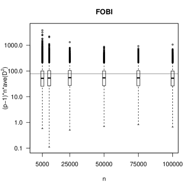
Figure 1: Boxplots for $n(p-1)\hat{D}^{2}$ based on the FOBI estimate for different sample sizes $n$ and 10000 repetitions on log scale. The three independent components have Laplace, logistic and $beta(3,3)$ distributions. The horizontal line gives the limiting mean value.

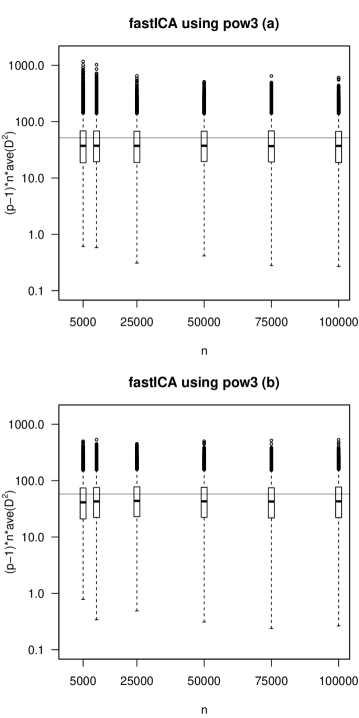
Figure 2: Boxplots for $n(p-1)\hat{D}^{2}$ based on the fastICA estimates pow3(a) and pow3(b) for different sample sizes $n$ and 10000 repetitions on log scale. The three independent components have Laplace, logistic and $beta(3,3)$ distributions. The horizontal line gives the limiting mean value.

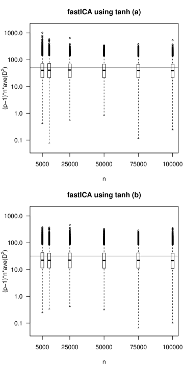
Figure 3: Boxplots for $n(p-1)\hat{D}^{2}$ based on the fastICA estimates tanh(a) and tanh(b) for different sample sizes $n$ and 10000 repetitions on log scale. The three independent components have Laplace, logistic and $beta(3,3)$ distributions. The horizontal line gives the limiting mean value.

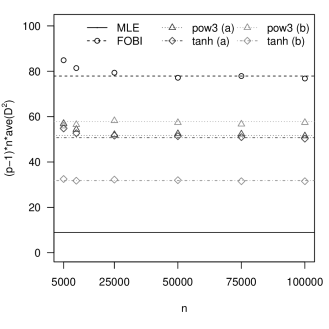
Figure 4: The estimated mean values of $n(p-1)\hat{D}^{2}$ for the estimates FOBI, pow3(a), pow3(b), tanh(a) and tanh(b). The dashed horizontal lines give the corresponding limiting mean values. The solid horizontal line is the limiting mean for the MLE (with known marginal distributions).

Boxplots in Figures 1, 2 and 3 illustrate the finite-sample behavior of the index for different estimates. The horizontal lines give the limiting mean values on a log scale. The FOBI estimate is known to converge in distribution to a multivariate normal distribution, but the convergence is very slow. The distributional convergence of $n(p-1)\hat{D}^{2}$ is then also slow as is seen from Figure 1. What is interesting, is that the speed of convergence of the distribution (not only the covariance structure) of the fastICA estimate seems to depend on the order of the found sources, see Figure 2 and Figure 3. The distributional convergence of $n(p-1)\hat{D}^{2}$ for tanh(b) seems to be faster than that for tanh(a), see Figure 3. The same is true for pow3(b) and pow3(a) as well, see Figure 2. The estimated means of $n(p-1)\hat{D}^{2}$ for different estimates $\hat{\Gamma}$ are compared in Figure 4 again with asymptotic horizontal lines. The performance of the FOBI estimate is clearly worst. The MLE with the assumption that the marginal distributions are known provides the Cramer-Rao lower bound for the limiting mean, see Ollila et al. (2008a). The order in which the sources are found seems to have a huge effect on the performance of the fastICA estimate. If the sources are found in the order $beta(3,3)$, logistic, and Laplace, there is no big difference between choices pow3: $g(z)=z^{3}$ and tanh: $g(z)=tanh(z)$. If the order is Laplace, logistic, and $beta(3,3),$ the estimate tanh perform very well while the estimate pow3 gets worse.

5 Summary

Independent component analysis (ICA) has gained increasing interest in various fields of applications in recent years. As far as we know, this paper provides the first rigorous (mathematical) definition of the IC functional. The functional is defined in a general semiparametric IC model and is independent from the parametrization of the model.

The deflation-based FastICA algorithm is one of the most popular ICA algorithms. Several superficial attempts to find the limiting distribution and limiting covariance matrix of the FastICA mixing matrix estimate can be found in the literature (see e.g. Tichavsky et al. (2005), Shimizu et al. (2006), Reyhani et al. (2012)). The correct limiting covariance matrix was found however quite recently in Ollila (2010). In this paper we provide the assumptions needed for the limiting multivariate normality.

For several popular ICA procedures, the statistical properties are still unknown, and their performances are compared using different performance criteria in simulation studies. In this paper we discuss several criteria in detail and suggest a new performance index with an easy interpretation. The asymptotic behavior of the new index depends in a natural way on the eigenvalues of the limiting covariance matrix of an unmixing matrix estimate. This is illustrated in a small simulation study with some deflation-based FastICA estimates and with FOBI estimate. We did not use other ICA procedures in our study as, for other estimates proposed in the literature, the limiting properties are still unknown and/or their implementations cannot deal with the sample sizes of our study. Note also that the new index can also be computed using the correlation matrix between the estimated and true sources. In that case the index has a nice connection to the mean-squared error as discussed in Nordhausen et al. (2011b).

The theory presented in this paper has also important practical implications. For example, Nordhausen et al. (2011d) introduces a new reloaded deflation-based FastICA algorithm that, using a preliminary estimate and the results here, extracts the sources in an optimal order to minimize the trace of the limiting covariance matrix.

Appendix

The Proof of Theorem 3.1

Assume that $\sqrt{n}\ \mathrm{vec}(\hat{G}-I_{p})\to_{d}N_{p^{2}}(0,\Sigma_{\Gamma})$. Now it follows directly from (Tan, 1977, Theorem 3.1) that the limiting distribution of $n\cdot D^{2}(\hat{G})$ is that of $\sum_{i=1}^{k}\delta_{i}\chi^{2}_{i}$ where $\chi^{2}_{1},....,\chi^{2}_{k}$ are independent chi squared variables with one degree of freedom, and $\delta_{1},...,\delta_{k}$ are the $k$ nonzero eigenvalues (including all algebraic multiplicities) of $\Sigma_{\Gamma}$.

The Proof of Theorem 3.2

For simplicity, we consider the elements $\hat{\Gamma}^{*}_{11}$ and $\hat{\Gamma}^{*}_{12}$ only. The proofs for other elements are similar. First note that

$$\sqrt{n}\left((\hat{\Gamma}\hat{S}\hat{\Gamma}^{\prime})_{11}-D_{11}^{-2}\right) = \sqrt{n}\left(\sum_{i=1}^{p}\sum_{j=1}^{p}\hat{\Gamma}_{1i}\hat{S}_{ij}\hat{\Gamma}_{1j}-D_{11}^{-2}\right)$$

$$= \sqrt{n}\left(2(\hat{\Gamma}_{11}-D_{11}^{-1})D_{11}^{-1}+(\hat{S}_{11}-1)D_{11}^{-2}\right)+o_{P}(1).$$

But then

$$\sqrt{n}\left((\hat{\Gamma}\hat{S}\hat{\Gamma}^{\prime})_{11}^{-1/2}-D_{11}\right)=-\sqrt{n}\left(D_{11}^{2}(\hat{\Gamma}_{11}-D_{11}^{-1})+\frac{D_{11}}{2}(\hat{S}_{11}-1)\right)+o_{P}(1)$$

and

$$\sqrt{n}(\hat{\Gamma}_{11}^{*}-1) = \sqrt{n}\left((\hat{\Gamma}\hat{S}\hat{\Gamma}^{\prime})_{11}^{-1/2}\hat{\Gamma}_{11}-1\right)$$

$$= \sqrt{n}\left(((\hat{\Gamma}\hat{S}\hat{\Gamma}^{\prime})_{11}^{-1/2}-D_{11})D_{11}^{-1}+D_{11}(\hat{\Gamma}_{11}-D_{11}^{-1})\right)$$

$$+o_{P}(1)$$

$$= -\frac{\sqrt{n}}{2}(\hat{S}_{11}-1)+o_{P}(1).$$

Finally,

$$\sqrt{n}\hat{\Gamma}_{12}^{*}=\sqrt{n}\left((\hat{\Gamma}\hat{S}\hat{\Gamma}^{\prime})_{11}^{-1/2}\hat{\Gamma}_{12}\right)=\sqrt{n}D_{11}^{-1}\hat{\Gamma}_{12}+o_{P}(1).$$

The Proof of Theorem 3.3

Assume that $\sqrt{n}\ \mathrm{vec}(\hat{G}-I_{p})\to_{d}N_{p^{2}}(0,\Sigma_{\Gamma^{*}})$, and let $D_{p,p}=\sum_{i=1}^{p}(e_{i}e_{i}^{T})\otimes(e_{i}e_{i}^{T})$. Now $\mathrm{vec}(\mbox{off}(\hat{G}))=(I_{p^{2}}-D_{p,p})\mathrm{vec}(\hat{G}-I_{p})$ and thus $\sqrt{n}\ \mathrm{vec}(\mbox{off}(\hat{G}))\to_{d}N_{p^{2}}(0,(I_{p^{2}}-D_{p,p})\Sigma_{\Gamma^{*}}(I_{p^{2}}-D_{p,p})).$ Now it follows from (Tan, 1977, Theorem 3.1) that the limiting distribution of $n||\mbox{off}(\hat{G})||^{2}$ is that of $\sum_{i=1}^{k}\delta_{i}\chi^{2}_{i}$ where $\chi^{2}_{1},....,\chi^{2}_{k}$ are independent chi squared variables with one degree of freedom, and $\delta_{1},...,\delta_{k}$ are the $k$ nonzero eigenvalues (including all algebraic multiplicities) of

$$(I_{p^{2}}-D_{p,p})\Sigma_{\Gamma^{*}}(I_{p^{2}}-D_{p,p}).$$

The Proof of Theorem 3.4

The proof follows from the fact that $\sqrt{n}(\hat{D}_{ii}\hat{G}_{ii}-1)=o_{P}(1)$. Then also $\sqrt{n}\hat{D}_{ii}\hat{G}_{ij}=\sqrt{n}D_{ii}\hat{G}_{ij}+o_{P}(1)$ for all $i\neq j$.

The Proof of Lemma 4.1

Let $A=(a_{ij})$ be a $p\times p$ matrix having at least one nonzero element in each row and let $\tilde{A}=(\tilde{a}_{ij})=\frac{a_{ij}^{2}}{\sum_{k=1}^{p}a_{ik}^{2}}.$ Let $\mathcal{L}$ denote the set of all nonsingular $p\times p$ diagonal matrices and let $L=(l_{ij})\in\mathcal{L}.$ Now

$$\|LA-I_{p}\|^{2}=\sum_{i=1}^{p}\sum_{j=1}^{p}l_{ii}^{2}a_{ij}^{2}-2\sum_{i=1}^{p}l_{ii}a_{ii}+p$$

and

$$\frac{\partial}{\partial l_{ii}}\|LA-I_{p}\|^{2}=2(l_{ii}\sum_{j=1}^{p}a_{ij}^{2}-a_{ii}).$$

The derivatives are zero with choices

$$l_{ii}=\frac{a_{ii}}{\sum_{j=1}^{p}a_{ij}^{2}}$$

and the value of $\|LA-I_{p}\|^{2}$ is then

$$p-\sum_{i=1}^{p}\frac{a_{ii}^{2}}{\sum_{j=1}^{p}a_{ij}^{2}}.$$

Let $\mathcal{P}$ denote the set of all $p\times p$ permutation matrices. Now it follows that if $\hat{G}=\hat{\Gamma}\Omega$, and $\tilde{G}_{ij}={\hat{G}_{ij}^{2}}/{\sum_{k=1}^{p}\hat{G}_{ik}^{2}}$, $i,j=1,...,p$, then the minimum distance index can be written as

$$\hat{D}=D(\hat{G})=\frac{1}{\sqrt{p-1}}\left(p-\max_{P\in\mathcal{P}}\left(\mbox{tr}(P\tilde{G})\right)\right)^{1/2}.$$

The Proof of Theorem 4.1

Let $A=(a_{ij})$ be a $p\times p$ matrix having at least one nonzero element in each row. Let $\tilde{A}=(\tilde{a}_{ij})$ with $\tilde{a}_{ij}=\frac{a_{ij}^{2}}{\sum_{k=1}^{p}a_{ik}^{2}}.$ Let $\mathcal{P}$ denote the set of all $p\times p$ permutation matrices. Now the shortest squared distance $D^{2}(A)=\frac{1}{p-1}(p-\max_{P\in\mathcal{P}}(\mbox{tr}(P\tilde{A}))).$ (See the proof of Lemma 4.1.) Consider now $\mbox{tr}(P\tilde{A}),$ where $\tilde{a}_{ij}\geq 0,$ for all $i,j$ and $\sum_{j=1}^{p}\tilde{a}_{ij}=1.$ Now clearly the maximum value of $\max_{P\in\mathcal{P}}\mbox{tr}(P\tilde{A})$ is $p$ and it is attained if and only if $\tilde{A}$ is a permutation matrix. Since $\tilde{A}$ is a permutation matrix if and only if $A\sim I_{p},$ we have now proven that $D^{2}(A)\geq 0$ for all $A$ and that $D^{2}(A)=0$ if and only if $A\sim I_{p}$.

For the minimum value of $\max_{P\in\mathcal{P}}\mbox{tr}(P\tilde{A})$ note that

$$\max_{P\in\mathcal{P}}\mbox{tr}(P\tilde{A})\geq\frac{1}{p!}\sum_{P\in\mathcal{P}}\mbox{tr}(P\tilde{A})=\frac{1}{p}\sum_{i=1}^{p}\sum_{j=1}^{p}\tilde{a}_{ij}=1.$$

If $\max_{P\in\mathcal{P}}\mbox{tr}(P\tilde{A})=1,$ then $\mbox{tr}(P\tilde{A})=1$ for all permutation matrices $P.$ Since all row sums of $\tilde{A}$ are one, if rows $i_{1}\neq i_{2}$ of $\tilde{A}$ are different, there have to exist indices $j_{1}\neq j_{2}$ such that $\tilde{a}_{i_{1}j_{1}}>\tilde{a}_{i_{2}j_{1}},$ and that $\tilde{a}_{i_{1}j_{2}}<\tilde{a}_{i_{2}j_{2}}.$ Let now $P_{1}$ and $P_{2}$ denote permutation matrices which are identical in all rows $i\not\in\{i_{1},i_{2}\}$ and in all columns $j\not\in\{j_{1},j_{2}\},$ and let the elements $i_{1}j_{1}$ and $i_{2}j_{2}$ of $P_{1}$ be equal to one, and let the elements $i_{1}j_{2}$ and $i_{2}j_{1}$ of $P_{2}$ be equal to one. Then $\mbox{tr}(P_{1}\tilde{A})>\mbox{tr}(P_{2}\tilde{A})$ contradicting the fact that $\mbox{tr}(P\tilde{A})$ is identical for all permutation matrices $P.$ Hence $A\sim 1_{p}a^{T}$ for some $p$-vector $a$. We have now proven that $1\geq D^{2}(A)$ for all $A$ and that $D^{2}(A)=1$ if and only if $A\sim 1_{p}a^{T}$ for some $p$-vector $a$.

Assume now that $a_{ij}\leq 1,i\neq j$ and let $B=I_{p}+c\ \mathrm{off}(A),$ where $c\in[0,1]$ and let $\tilde{B}=(\tilde{b}_{ij})=\frac{b_{ij}^{2}}{\sum_{k=1}^{p}b_{ik}^{2}}$. Then $\max_{P}\mbox{tr}(P\tilde{B})=\sum_{i=1}^{p}\frac{1}{c^{2}\sum_{j=1,j\neq i}^{p}a_{ij}^{2}+1}.$ Now clearly $\max_{P}\mbox{tr}(P\tilde{B})$ decreases when $c$ increases. This proves that the function $c\to D^{2}(I_{p}+c\ \mathrm{off}(A))$ is increasing in $c\in[0,1]$ for all matrices $A$ such that $A_{ij}^{2}\leq 1$, $i\neq j$.

The Proof of Theorem 4.2

Let $\Gamma(F_{x})=\Omega=C(F_{x})=I_{p}$ and let $\sqrt{n}\ \mathrm{vec}(\hat{\Gamma}-I_{p})\to_{d}N_{p^{2}}(0,\Sigma)$. Let $\mathcal{P}$ denote the set of all $p\times p$ permutation matrices and let $\mathcal{L}$ denote the set of all nonsingular $p\times p$ diagonal matrices.

We have

$$\hat{D}=\frac{1}{\sqrt{p-1}}\inf_{C\in\mathcal{C}}\|C\hat{\Gamma}-I_{p}\|=\frac{1}{\sqrt{p-1}}\min_{P\in\mathcal{P}}(\inf_{L\in\mathcal{L}}\|LP\hat{\Gamma}-I_{p}\|).$$

Let

$$\hat{P}_{m}=\mathrm{argmin}_{P\in\mathcal{P}}(\inf_{L\in\mathcal{L}}\|LP\hat{\Gamma}-I_{p}\|),\ \hat{L}_{m}=\mathrm{arginf}_{L\in\mathcal{L}}\|L\hat{P}_{m}\hat{\Gamma}-I_{p}\|,$$

$$P_{m}=\mathrm{argmin}_{P\in\mathcal{P}}(\inf_{L\in\mathcal{L}}\|LP\Gamma-I_{p}\|),\ L_{m}=\mathrm{arginf}_{L\in\mathcal{L}}\|LP_{m}\Gamma-I_{p}\|$$

and for all $P\in\mathcal{P}$ let $\hat{L}_{P}=\mathrm{arginf}_{L\in\mathcal{L}}\|LP\hat{\Gamma}-I_{p}\|$ and $L_{P}=\mathrm{arginf}_{L\in\mathcal{L}}\|LP\Gamma-I_{p}\|.$ Now for all $P\in\mathcal{P},$ $(\hat{L}_{P})_{ii}=\hat{B}_{ii}/\sum_{j=1}^{p}\hat{B}_{ij}^{2},$ where $\hat{B}_{ij}=(\hat{B}_{P})_{ij}=(P\hat{\Gamma})_{ij}$ and $(L_{P})_{ii}=B_{ii}/\sum_{j=1}^{p}B_{ij}^{2},$ where $B_{ij}=(B_{P})_{ij}=(P\Gamma)_{ij},$ (see the proof of Lemma 4.1). Let $P\in\mathcal{P}.$ Since $(\hat{\Gamma}-\Gamma)\stackrel{{\scriptstyle P}}{{\rightarrow}}\bar{0},$ it now follows from the continuous mapping theorem that also $(P\hat{\Gamma}-P\Gamma)\stackrel{{\scriptstyle P}}{{\rightarrow}}\bar{0}$ and thus $(\hat{L}_{P}-L_{P})\stackrel{{\scriptstyle P}}{{\rightarrow}}\bar{0}.$ Since $(\hat{L}_{P}-L_{P})\stackrel{{\scriptstyle P}}{{\rightarrow}}\bar{0}$ holds for all $P\in\mathcal{P},$ it follows that $(\hat{P}_{m}-P_{m})\stackrel{{\scriptstyle P}}{{\rightarrow}}\bar{0}$ and $(\hat{L}_{m}-L_{m})\stackrel{{\scriptstyle P}}{{\rightarrow}}\bar{0}$ as well.

Clearly

$$P_{m}=L_{m}=I_{p}.$$

Since $P_{m}$ and $\hat{P}_{m}$ are discrete, we now have, by using Slutsky’s theorem, that

$$\sqrt{n}\ \mathrm{vec}(\hat{L}_{m}\hat{P}_{m}\hat{\Gamma}-I_{p})=\sqrt{n}\ \mathrm{vec}(\hat{L}_{m}-I_{p})+\sqrt{n}\ \mathrm{vec}(\hat{\Gamma}-I_{p})+o_{P}(1).$$

Consider now

$$\sqrt{n}\ \mathrm{vec}(\hat{L}_{m}-I_{p}).$$

Let $\hat{A}=(\hat{a}_{ij})=\hat{P}_{m}\hat{\Gamma}$ and define diagonal matrices $\hat{D}_{a}=(\hat{D}_{a})_{ii}=\hat{a}_{ii},$ $\hat{D}_{b}=(\hat{D}_{b})_{ii}=\frac{1}{\sum_{j=1}^{p}\hat{a}_{ij}^{2}}.$ Now

$$\sqrt{n}(\hat{L}_{m}-I_{p})=\sqrt{n}(\hat{D}_{a}-I_{p})\hat{D}_{b}+\sqrt{n}(\hat{D}_{b}-I_{p})$$

and it follows from the convergency of $\hat{P}_{m}$ and $\hat{\Gamma}$ that $(\hat{D}_{a}-I_{p})\stackrel{{\scriptstyle P}}{{\rightarrow}}\bar{0}$ and $(\hat{D}_{b}-I_{p})\stackrel{{\scriptstyle P}}{{\rightarrow}}\bar{0}.$

Consider now the $ii$ element of the matrix $\sqrt{n}(\hat{D}_{b}-I_{p}).$ We have $\sqrt{n}(\frac{1}{\sum_{j=1}^{p}\hat{a}_{ij}^{2}}-1)=\sqrt{n}\frac{1-\sum_{j=1}^{p}\hat{a}_{ij}^{2}}{\sum_{j=1}^{p}\hat{a}_{ij}^{2}}.$ It now follows from our assumptions and discreteness of $\hat{P}_{m}$ and $P_{m}$ that each $\sqrt{n}\hat{a}_{ij},\ i\neq j$ converges to normal distribution with zero mean. Now each $n\hat{a}_{ij}^{2},\ i\neq j$ converges in distribution to a $\chi^{2}$ variable and thus each $\sqrt{n}\hat{a}_{ij}^{2},\ i\neq j$ converges in probability to zero and $(\sqrt{n}\frac{1-\sum_{j=1}^{p}\hat{a}_{ij}^{2}}{\sum_{j=1}^{p}\hat{a}_{ij}^{2}}-\sqrt{n}\frac{1-\hat{a}_{ii}^{2}}{\sum_{j=1}^{p}\hat{a}_{ij}^{2}})$ $=(\sqrt{n}\frac{1-\sum_{j=1}^{p}\hat{a}_{ij}^{2}}{\sum_{j=1}^{p}\hat{a}_{ij}^{2}}-(\frac{1+\hat{a}_{ii}}{-\sum_{j=1}^{p}\hat{a}_{ij}^{2}}(\sqrt{n}(\hat{a}_{ii}-1))))$ converges in probability to zero as well. Now since $\frac{1+\hat{a}_{ii}}{-\sum_{j=1}^{p}\hat{a}_{ij}^{2}}=-2+o_{P}(1),$ it follows from Slutsky’s theorem that

$$\sqrt{n}\ \mathrm{vec}(\hat{L}_{m}-I_{p})=-\sqrt{n}\ \mathrm{vec}(\hat{D}_{a}-I_{p})+o_{P}(1).$$

Since $(\hat{\Gamma}-I_{p})=(\hat{P}_{m}\hat{\Gamma}-I_{p})+((\hat{P}_{m}-I_{p})\hat{\Gamma})$, we now have by Slutsky’s theorem and discreteness of $\hat{P}_{m}$ that

$$\sqrt{n}\mathrm{diag}(\hat{\Gamma}-I_{p})=\sqrt{n}\mathrm{diag}(\hat{P}_{m}\hat{\Gamma}-I_{p})+o_{P}(1).$$

Since

$$\sqrt{n}(\hat{D}_{a}-I_{p})=\sqrt{n}\mathrm{diag}(\hat{P}_{m}\hat{\Gamma}-I_{p}),$$

we conclude, using Slutsky’s theorem again, that

$$\sqrt{n}\ \mathrm{vec}(\hat{L}_{m}\hat{P}_{m}\hat{\Gamma}-I_{p})\stackrel{{\scriptstyle d}}{{\rightarrow}}N(\bar{0},\Sigma_{2}),$$

where

$$\Sigma_{2}=ASCOV(\sqrt{n}\ \mbox{vec}(\mathrm{off}(\hat{\mathrm{\Gamma}})))=(I_{p^{2}}-D_{p,p})\Sigma(I_{p^{2}}-D_{p,p})$$

with $D_{p,p}=\sum_{i=1}^{p}(e_{i}e_{i}^{T})\otimes(e_{i}e_{i}^{T})$. Thus

$$n\hat{D}^{2}=\frac{n}{p-1}\|\mathrm{off}(\hat{\Gamma})\|^{2}+o_{P}(1)$$

and it follows from (Tan, 1977, Theorem 3.1), that the limiting distribution of $n\hat{D}^{2}$ is that of $(p-1)^{-1}\sum_{i=1}^{k}\delta_{i}\chi^{2}_{i}$ where $\chi^{2}_{1},....,\chi^{2}_{k}$ are independent chi squared variables with one degree of freedom, and $\delta_{1},...,\delta_{k}$ are the $k$ nonzero eigenvalues (including all algebraic multiplicities) of $\Sigma_{2}.$

References

• Amari et al. (1996) Amari, S.Β I., Cichocki, A. and Yang H.Β H. (1996) A new learning algorithm for blind source separation. Advances in Neural Information Processing Systems 8, 757–763.
• Brys et al. (2006) Brys, G., Hubert, M. and Rousseeuw, P.J. (2006) A robustification of independent component analysis. Chemometrics 57(19), 364–375.
• Bugrien (2005) Bugrien, J. (2005) Robust approaches to clustering based on density estimation and projection. PhD thesis, University of Leeds.
• Cardoso and Souloumiac (1993) Cardoso, J.F., Souloumiac, A. (1993) Blind beamforming for non Gaussian signals. IEEE Proceedings-F 140, 362–370.
• Cardoso (1989) Cardoso, J.F. (1989) Source separation using higher moments. Proceedings of IEEE international conference on acustics, speech and signal processing, 2109–2112.
• Chen and Bickel (2005) Chen, A. and Bickel, P.J. (2005) Consistent independent component anlysis and prewithening. IEEE Transactions on Signal Processing 53, 3625–3631.
• Chen and Bickel (2006) Chen, A. and Bickel, P.J. (2006) Efficient independent component analysis. The Annals of Statistics 34, 2825–2855.
• Cichocki and Amari (2006) Cichocki, A. and Amari, S.Β I. (2006) Adaptive Blind Signal and Image Processing. John Wiley & Sons, Chichester.
• Dantzig and Thapa (1997) Dantzig, G.Β B. and Thapa, M.Β N. (1997) Linear Programming 1: Introduction. Springer, New York.
• Douglas (2007) Douglas, S.Β C. (2007) Fixed-point algorithms for the blind separation of arbitrary complex-valued non-gaussian signal mixtures. EURASIP Journal on Advances in Signal Processing 1, 83–83.
• HyvΓ€rinen and Oja (1997) HyvΓ€rinen, A. and Oja, E. (1997) A fast fixed-point algorithm for independent component analysis. Neural Computation 9, 1483–1492.
• HyvΓ€rinen et al. (2001) HyvΓ€rinen, A., Karhunen, J. and Oja, E. (2001) Independent Component Analysis. John Wiley & Sons, New York.
• Ilmonen (2012) Ilmonen, P. (2012) On asymptotical properties of the scatter matrix based estimates for complex valued independent component analysis. Submitted.
• Ilmonen et al. (2010a) Ilmonen, P., Nevalainen, J. and Oja, H. (2010a) Characteristics of multivariate distributions and the invariant coordinate system. Statistics and Probability Letters 80, 1844–1853.
• Ilmonen et al. (2010b) Ilmonen, P., Nordhausen, K., Oja, H. and Ollila, E. (2010b) A new performance index for ICA: properties, computation and asymptotic analysis, Latent Variable Analysis and Signal Processing (IEEE Proceedings of 9th International Conference on Latent Variable Analysis and Signal Separation), 229–236.
• Ilmonen et al. (2012) Ilmonen, P., Oja, H. and Serfling, R. (2012) On invariant coordinate system (ICS) functionals. International Statistical Review 80(1), 93–110.
• Ilmonen and Paindaveine (2011) Ilmonen, P., and Paindaveine, D. (2011) Semiparametrically efficient inference based on signed ranks in symmetric independent component models. The Annals of Statistics 39(5), 2448–2476.
• Moreau and Macchi (1994) Moreau, E. and Macchi, O. (1994) A one stage self-adaptive algorithm for source separation. IEEE International Conference on Acoustics, Speech and Signal Processing, Adelaide, Australia, 49–52.
• Nordhausen et al. (2008) Nordhausen, K., Oja, H. and Ollila, E. (2008) Robust independent component analysis based on two scatter matrices. Austrian Journal of Statistics 37, 91–100.
• Nordhausen et al. (2011a) Nordhausen, K., Oja, H. and Ollila, E. (2011a) Multivariate models and the first four moments. In Hunter, D.R., Richards, D.S.R. and Rosenberger, J.L. (editors) Nonparametric Statistics and Mixture Models: A Festschrift in Honor of Thomas P. Hettmansperger, 267–287, World Scientific, Singapore.
• Nordhausen et al. (2011b) Nordhausen, K., Ollila, E. and Oja, H. (2011b) On the performance indices of ICA and blind source separation. In proceedings of 2011 IEEE 12th International Workshop on Signal Processing Advances in Wireless Communications (SPAWC 2011), 171–175.
• Nordhausen et al. (2011c) Nordhausen, K., Cardoso, J.F., Oja, H. and Ollila, E. (2011c) JADE and ICA performance criteria. R package version 1.0-4.
• Nordhausen et al. (2011d) Nordhausen, K., Ilmonen, P., Mandal, A., Oja, H. and Ollila, E. (2011d) Deflation-based FastICA reloaded. In the Proceedings of 19th European Signal Processing Conference 2011 (EUSIPCO 2011), 1854–1858.
• Oja et al (2006) Oja, H., SirkiΓ€, S. and Eriksson, J. (2006) Scatter matrices and independent component analysis. Austrian Journal of Statistics 35, 175–189.
• Ollila (2010) Ollila, E. (2010) The deflation-based FastICA estimator: statistical analysis revisited. IEEE Transactions in Signal Processing 58, 1527–1541.
• Ollila et al. (2008a) Ollila, E., Kim, H.-J. and Koivunen, V. (2008a) Compact Cramer-Rao bound expression for independent component analysis. IEEE Transactions on Signal Processing 56, 1421–1428.
• Ollila et al. (2008b) Ollila, E., Oja, H. and Koivunen, V. (2008b) Complex-valued ICA based on a pair of generalized covariance matrices. Computational Statistics & Data Analysis 52, 3789–3805.
• Papadimitriou and Steiglitz (1982) Papadimitriou, C. and Steiglitz, K. (1982) Combinatorial Optimization: Algorithms and Complexity. Englewood Cliffs, Prentice Hall.
• Reyhani et al. (2012) Reyhani, N., Ylipaavalniemi, J., Vigario, R. and Erkki, O. (2012) Consistency and asymptotic normality of FastICA and bootstrap FastICA. Signal Processing 92, 1767–1778.
• Roelandt et al. (2009) Roelandt, E., Van Aelst, S. and Croux, C. (2009) Multivariate Generalized S-estimators. Journal of Multivariate Analysis 100, 876–887.
• Shimizu et al. (2006) Shimizu, S., HyvΓ€rinen, A., Kano, Y., Hoyer, P.Β O. and Kerminen, A.Β J. (2006) Testing significance of mixing and demixing coefficients in ICA. Proceedings of International Symposium on Independent Component Analysis and Blind Signal Separation (ICA2006), Charleston, SC, USA.
• SirkiΓ€ et al. (2007) SirkiΓ€, S., Taskinen, S., and Oja, H. (2007) Symmetrized M-estimators of scatter. Journal of Multivariate Analysis 98, 1611–1629.
• Tan (1977) Tan, W. Y. (1977) On the Distribution of Quadratic Forms in Normal Random Variables, The Canadian Journal of Statistics 5, 241–250.
• Theis et al. (2004) Theis, F.Β J., Lang, E.Β W. and Puntonet, C.Β G. (2004) A geometric algorithm for overcomplete linear ICA. Neurocomputing 56, 381–398.
• Tichavsky et al. (2005) Tichavsky, P., Koldovsky, Z. and Oja, E. (2005) Asymptotic performance of the fastica algorithm for independent component analysis and its iprovements, in proceedins of 2005 IEEE/SP 13th Workshop on Statistical Signal Processing, 1084–1089.
• Tyler et al. (2009) Tyler, D.Β E., Critchley, F., DΓΌmbgen, L. and Oja, H. (2009) Invariant coordinate selection. Journal of Royal Statistical Society, Series B 71, 549–592.
• Yeredor (2009) Yeredor, A. (2009) On Optimal Selection of Correlation Matrices for Matrix-Pencil-Based Separation. Lecture Notes in Computer Science (LNCS 5441): Independent Component analysis and Signal Separation, 8th International Conference on ICA, Paraty, Brazil, Springer-Verlag , Berlin Heidelberg.