Anomalous scaling of a passive vector field in $d$ dimensions: Higher-order structure functions

Abstract

The problem of anomalous scaling in the model of a transverse vector field $\theta_{i}(t,{\bf x})$ passively advected by the non-Gaussian, correlated in time turbulent velocity field governed by the Navier–Stokes equation, is studied by means of the field-theoretic renormalization group and operator product expansion. The anomalous exponents of the $2n$-th order structure function $S_{2n}(r)=\langle[\theta(t,{\bf x})-\theta(t,{\bf x}+{\bf r})]^{2n}\rangle$, where $\theta$ is the component of the vector field parallel to the separation ${\bf r}$, are determined by the critical dimensions of the family of composite fields (operators) of the form $(\partial\theta\partial\theta)^{2n}$, which mix heavily in renormalization. The daunting task of the calculation of the matrices of their critical dimensions (whose eigenvalues determine the anomalous exponents) simplifies drastically in the limit of high spatial dimension, $d\to\infty$. This allowed us to find the leading and correction anomalous exponents for the structure functions up to the order $S_{56}$. They reveal intriguing regularities, which suggest for the anomalous exponents simple “empiric” formulae that become practically exact for $n$ large enough. Along with the explicit results for smaller $n$, they provide the full description of the anomalous scaling in the model. Key words: passive vector field, turbulent advection, anomalous scaling, renormalization group, operator product expansion.

1 Introduction

In the past two decades, much attention has been attracted by turbulent advection of passive scalar fields; see the review paper [1] and references therein. Being of practical importance in itself, the problem of passive advection can be viewed as a starting point for studying intermittency and anomalous scaling in the fluid turbulence on the whole [2]. Most progress was achieved for the so-called Kraichnan’s rapid-change model, in which the advecting velocity field $v_{i}(x)$ with $x=\{t,{\bf x}\}$ is modelled by a Gaussian statistics with vanishing correlation time and prescribed correlation function $\langle vv\rangle\propto\delta(t-t^{\prime})k^{-d-\xi}$, where $k$ is the wave number, $d$ is the dimension of space and $\xi$ is an arbitrary exponent with the most realistic (Kolmogorov) value $\xi=4/3$. The structure functions of the advected scalar field $\theta(x)$ in the inertial range demonstrate anomalous scaling behaviour:

$$S_{2n}(r)=\big{\langle}[\theta(t,{\bf x})-\theta(t,{\bf x^{\prime}})]^{2n}\big{\rangle}\propto r^{n(2-\xi)}\,(r/L)^{\Delta_{n}},$$ (1.1)

that is, singular dependence on the separation $r=|{\bf r}|$ (where ${\bf r}={\bf x}-{\bf x^{\prime}}$) and on the integral turbulence scale $L$, characterized by an infinite set of the exponents $\Delta_{n}$. Within the framework of the so-called zero-mode approach, these exponents were calculated in the leading order of the expansions in $\xi$ [3] and $1/d$ [4]:

$$\Delta_{n}=-2n(n-1)\xi/(d+2)+O(\xi^{2})=-2n(n-1)\xi/d+O(1/d^{2}).$$ (1.2)

In [5] and subsequent papers, the field theoretic renormalization group (RG) and the operator product expansion (OPE) were applied to Kraichnan’s model; see [6] for a review and the references. In that approach, the anomalous scaling emerges as a consequence of the existence in the corresponding OPE of certain composite fields (“operators” in the quantum-field terminology) with negative dimensions, which are identified with the anomalous exponents $\Delta_{n}$. This allows one to construct a systematic perturbation expansion for the anomalous exponents and to calculate them up to the orders $\xi^{2}$ [5] and $\xi^{3}$ [7]. Besides the calculational efficiency, an important advantage of the RG+OPE approach is its relative universality: it can also be applied to the case of finite correlation time or non-Gaussian advecting fields. For passively advected vector fields, any calculation of the exponents for higher-order correlations calls for the RG techniques already in the $O(\xi)$ approximation.

In this paper, we study anomalous scaling of a passive vector quantity, advected by a non-Gaussian velocity field, governed by the stirred Navier–Stokes (NS) equation. For the rapid-change velocity ensemble, a similar model was introduced and thoroughly studied in [8]–[12]; effects of finite correlation time and weak anisotropy were studied in [13]. Before explaining our motivations, which follow the same lines as those of refs. [8, 10, 11], let us discuss the definition of the model.

We confine ourselves with the case of transverse (divergence-free) passive $\theta_{i}(x)$ and advecting $v_{i}(x)$ vector fields. Then the general advection-diffusion equation has the form

$$\nabla_{t}\theta_{i}-{\cal A}(\theta_{k}\partial_{k})v_{i}+\partial_{i}{\cal P}=\kappa_{0}\partial^{2}\theta_{i}+\eta_{i},\qquad\nabla_{t}\equiv\partial_{t}+(v_{k}\partial_{k}),$$ (1.3)

where $\nabla_{t}$ is the Lagrangian (Galilean covariant) derivative, ${\cal P}(x)$ is the pressure, $\kappa_{0}$ is the diffusivity, $\partial^{2}$ is the Laplace operator and $\eta_{i}(x)$ is a transverse Gaussian stirring force with zero mean and covariance

$$\langle\eta_{i}(x)\eta_{k}(x^{\prime})\rangle=\delta(t-t^{\prime})\,C_{ik}(r/L).$$ (1.4)

The parameter $L$ is an integral scale related to the stirring, and $C_{ik}$ is a dimensionless function, finite at $r=0$ and rapidly decaying for $r\to\infty$; its precise form is unimportant. Due to the transversality conditions $\partial_{i}\theta_{i}=\partial_{i}v_{i}=0$, the pressure can be expressed as the solution of the Poisson equation,

$$\partial^{2}{\cal P}=({\cal A}-1)\,\partial_{i}v_{k}\partial_{k}\theta_{i}.$$ (1.5)

Thus the pressure term makes the dynamics (1.3) consistent with the transversality. The amplitude factor ${\cal A}$ in front of the “stretching term” $(\theta_{k}\partial_{k})v_{i}$ is not fixed by the Galilean symmetry and thus can be arbitrary. Such general “${\cal A}$ model” was introduced and studied in refs. [14]. The most popular special case ${\cal A}=1$, where the pressure term disappears, corresponds to magnetohydrodynamic turbulence. It was studied earlier in numerous papers; see e.g. refs. [15] and references therein.

In earlier studies, the velocity field in (1.3) was described by the Kraichnan’s rapid-change model. In this paper, we employ the stochastic NS equation:

$$\nabla_{t}v_{i}=\nu_{0}\partial^{2}v_{i}-\partial_{i}{\wp}+f_{i},$$ (1.6)

where $\nabla_{t}$ is the same Lagrangian derivative, ${\wp}$ and $f_{i}$ are the pressure and the transverse random force per unit mass. We assume for $f$ a Gaussian distribution with zero mean and correlation function

$$\big{\langle}f_{i}(x)f_{j}(x^{\prime})\big{\rangle}=\frac{\delta(t-t^{\prime})}{(2\pi)^{d}}\,\int_{k\geq m}d{\bf k}\,P_{ij}({\bf k})\,d_{f}(k)\,\exp\big{[}{\rm i}{\bf k}\left({\bf x}-{\bf x}^{\prime}\right)\big{]},$$ (1.7)

where $P_{ij}({\bf k})=\delta_{ij}-k_{i}k_{j}/k^{2}$ is the transverse projector, $d_{f}(k)$ is some function of $k\equiv|{\bf k}|$ and model parameters. The momentum $m=1/L$, the reciprocal of the integral scale $L$ related to the velocity, provides IR regularization. For simplicity, we do not distinguish it from the integral scale related to the scalar noise in (1.4).

The standard RG formalism is applicable to the problem (1.6), (1.7) if the correlation function of the random force is chosen in the power form [16]

$$d_{f}(k)=D_{0}\,k^{4-d-y},$$ (1.8)

where $D_{0}>0$ is the positive amplitude factor and the exponent $0<y\leq 4$ plays the role of the RG expansion parameter. The most realistic value of the exponent is $y=4$: with an appropriate choice of the amplitude, the function (1.8) for $y\to 4$ turns to the delta function, $d_{f}(k)\propto\delta({\bf k})$, which corresponds to the injection of energy to the system owing to interaction with the largest turbulent eddies; for a more detailed justification see e.g. [17, 18].

In this paper we consider the model (1.3) without the stretching term, that is, ${\cal A}=0$. Being formally a special case of the general ${\cal A}$ model, it appears exceptional in a few respects and requires special attention [8]–[13].

The feature specific only of the ${\cal A}=0$ is the symmetry with respect to the shift $\theta\to\theta+{\rm const}$, because only derivatives of the field $\theta$ enter the equation (1.3). The quantities of interest are the structure functions (1.1), in which $\theta$ should be understood as the component of the vector field parallel to the separation, $\theta=\theta_{i}r_{i}/r$: in contrast to ordinary correlation functions, they are also invariant with respect to the shift. As a consequence, all the composite operators that enter the corresponding OPE, should also be invariant, that is, built only of the derivatives of $\theta$.

For the scalar problem, the operator that determines the leading term of the inertial-range asymptotic behaviour (1.1), is unique: it has the form $(\partial_{i}\theta\partial_{i}\theta)^{n}$, the $n$-th power of the local dissipation rate of the scalar field fluctuations, and its critical dimension gives the anomalous exponent $\Delta_{n}$ is (1.2); see [5]–[7] for the detailed discussion.

For the vector case one can construct many scalar operators of the form $(\partial\theta)^{2n}$ for a given $n$, and in order to find the corresponding set of exponents and to identify the leading contribution, one has to consider the renormalization of the whole family, which implies the mixing of individual operators [8, 10]. Renormalization of families of mixing composite fields and calculation of the corresponding matrices of critical dimensions (whose eigenvalues give the desired anomalous exponents) its rather cumbersome and labor-consuming task, which should be solved separately for different families (in the case at hand, for different $n$). Thus, at first sight, there is no hope to derive simple explicit expressions for the anomalous exponents, similar to (1.2) in the scalar case.

In this respect, the ${\cal A}=0$ case of the model (1.3) resembles the nonlinear stirred NS equation, where the inertial-range behavior of structure functions is believed to be related with the Galilean-invariant (and hence built of the velocity gradients) operators, which mix heavily in renormalization; see [17] and references therein. In that case, the full solution is not yet obtained even for the relatively simple case of the family that includes the square of the energy dissipation rate [19].

Thus the ${\cal A}=0$ vector model (1.3) is of special interest: it also involves the problem of mixing, but now the problem is not a hopeless one: the leading terms are determined by finite families of composite operators, namely, those of the form $(\partial\theta)^{2n}$ with all possible contractions of vector indices, and such families with a given $n$ are closed with respect to the renormalization [8, 10]. What is more, for low values of $d$ there are linear relations between the operators, which reduce drastically the number of independent monomials [12]. As a result, the leading anomalous exponents for $d=2$ were calculated to the order $O(\xi^{2})$ for all $n$, and for $d=3$ – to the order $O(\xi)$ for $n\leq 9$ [12]. Crucial simplifications also take place in the limit $d\to\infty$ [10]: like for the scalar Kraichnan’s model, the anomalous exponents decay as $O(1/d)$ for large $d$, so that the anomalous scaling disappears at $d=\infty$; cf. (1.2). In order to find the leading exponents (and the closest corrections) it is sufficient to consider some special subset of the whole family $(\partial\theta)^{2n}$, and the corresponding matrix of critical dimensions can be built by a simple algorithm [10]. This allowed us to find all the negative dimensions in the leading order of the double expansion in $\xi$ and $1/d$ for $n$ as large as $n=28$, which gives the anomalous exponents and the close corrections for the structure functions up to $S_{56}$ [11]. All those results, however, refer to the Gaussian velocity field.

For very large $n$ the calculations become too labor- and time consuming (mostly due to the diagonalization of the matrices), but they are not necessary: the large-$n$ results suggest some simple empiric explicit expressions for the leading, next-to-leading, etc, anomalous exponents, which become practically exact as $n$ increases. Along with the explicit answers for smaller $n$, this gives the complete description of the anomalous scaling in the vector model for all $n$ and large $d$ [11].

It should be emphasized that the study of the large-$d$ behaviour of the fluid turbulence is by no means of only academic interest. It is related to the old idea of the expansion in $1/d$, which has repeatedly been introduced in various contexts [20]–[25].

The problem is that the ordinary perturbation theory for the stirred (stochastic) NS equation (that is, the perturbation expansion in the nonlinearity) is in fact an expansion in the Reynolds number, a parameter which tends to infinity for the fully developed turbulence. A similar problem is well known in the theory of critical state, where it is solved by means of the RG techniques; see e.g. [18]. The RG allows one to rearrange (to sum up) the plain perturbation series and to replace them with the famous $\varepsilon$ expansion, where $\varepsilon=4-d$ is the deviation of the spatial dimension $d$ from its upper critical value $d=4$. The turbulence (or, better to say, the corresponding stochastic models), has no upper critical dimension, and the RG expansion parameter has completely different meaning. As already mentioned, in Kraichnan’s model its role is played by the exponent $\xi$, while in the RG approach to the stirred NS equation its analog is the exponent $y$ in the correlator of the stirring force; see section 2. The results of the RG analysis of this model are reliable and internally consistent for asymptotically small $\xi$ or $y$, while the possibility of their extrapolation to the physical finite values, and thus their relevance for the real fluid turbulence, is sometimes called in question; see the discussion and the references in [25, 26].

One can hope that in the limit $d\to\infty$ intermittency and anomalous scaling disappear or acquire a simple “calculable” form and the finite-dimensional turbulence can be studied within the expansion around this “solvable” limit [21]. Indeed, it was argued (on the basis of a certain SDE-motivated ansatz for dissipative terms) that the Kolmogorov theory becomes exact and the multiscaling indeed disappears for $d=\infty$ [22], as it also happens for the Obukhov–Kraichnan model [20]. What is more, for the latter it was possible to find the $O(1/d)$ contribution to the anomalous exponents [4]; see the last expression in (1.2). However, the systematic expansion in $1/d$ has not been yet constructed for that model, let alone the stochastic NS equation.

It was suggested in [24, 25] that new progress can be achieved by combining the large-$d$ limit with the RG approach and the expansion in $\varepsilon$. In particular, it was noticed [10, 24] that taking the limit $d\to\infty$ leads to serious simplifications in the RG calculations, especially for composite operators. In a very important paper [24], scaling dimensions of all the powers of the local energy dissipation rate for the NS problem were calculated for $d=\infty$ to first order in $y$, the problem that looks unfeasible for finite $d$; see the discussion in [19].

Thus the drastic simplifications that occur in our vector model with the turbulent mixing provided by the NS velocity field and the simple explicit results for the anomalous dimensions in the leading order of the double expansion in $y$ and $1/d$, give a new strong support to the idea of the large-$d$ expansion.

The plan of the paper is as follows. In sec. 2 we discuss the field theoretic formulation of our stochastic problem and its renormalization. We show that the corresponding RG equations have an IR attractive fixed point, which implies existence of IR scaling behaviour for various correlation functions. In sec. 3, inertial-range anomalous scaling of the structure functions is studied by means of the OPE and the role of the operators $(\partial\theta)^{2n}$ is clarified. In sec. 4 we discuss the renormalization of those operators and the simplifications that occur in the limit of large $d$. Examples are given of the matrices of critical dimensions for a few families of those operators. In sec. 5 the leading and correction anomalous exponents, determined by the eigenvalues of those matrices, are presented and the regularities that they reveal are discussed. These regularities suggest for the eigenvalues some simple “empiric” formulae that become practically exact for $n$ large enough. Along with the explicit results obtained for smaller $n$, they provide the full description of the anomalous scaling in the present model. Sec. 6 is reserved for a brief conclusion.

2 Field theoretic formulation, renormalization and RG equations

According to the general theorem (see e.g. [18]), the full-scale stochastic problem (1.3)–(1.8) for ${\cal A}=0$ is equivalent to the field theoretic model of the doubled set of fields $\Phi=\{v,v^{\prime},\theta,\theta^{\prime}\}$ with the action functional

$${\cal S}(\Phi)={\cal S}_{v}({\bf v}^{\prime},{\bf v})+\theta^{\prime}D_{\theta}\theta^{\prime}/2+\theta^{\prime}\left\{-\nabla_{t}+\kappa_{0}\partial^{2}\right\}\theta,$$ (2.1)

where $D_{\theta}$ is the correlation function (1.4) of the random noise $f$ in (1.3) and $S_{v}$ is the action for the problem (1.6)–(1.8):

$${\cal S}_{v}({\bf v}^{\prime},{\bf v})=v^{\prime}D_{v}v^{\prime}/2+v^{\prime}\left\{-\nabla_{t}+\nu_{0}\partial^{2}\right\}v,$$ (2.2)

where $D_{v}$ is the correlation function (1.7) of the random force $f_{i}$. All the integrations over $x=\{t,{\bf x}\}$ and summations over the vector indices are understood. The auxiliary vector fields $v^{\prime},\theta^{\prime}$ are also transverse, $\partial_{i}v_{i}^{\prime}=\partial_{i}\theta_{i}^{\prime}=0$, which allows to omit the pressure terms on the right-hand sides of expressions (2.1), (2.2), as becomes evident after the integration by parts. For example,

$$\int dt\int d{\bf x}\ v_{i}^{\prime}\partial_{i}{\wp}=-\int dt\int d{\bf x}\ {\wp}(\partial_{i}v_{i}^{\prime})=0.$$

Of course, this does not mean that the pressure contributions are unimportant: the fields $v^{\prime},\theta^{\prime}$ act as transverse projectors and select the transverse parts of the expressions to which they are contracted.

The role of the coupling constants is played by the two parameters $g_{0}\equiv D_{0}/\nu_{0}^{3}$ and $u_{0}=\kappa_{0}/\nu_{0}$, the analog of the inverse Prandtl number in the scalar case. By dimension,

$$g_{0}\propto\Lambda^{y}\quad{\rm and}\quad u_{0}\propto\Lambda^{0},$$ (2.3)

where $\Lambda$ is the characteristic ultraviolet (UV) momentum scale. Thus the model (2.1), (2.2) becomes logarithmic (both the coupling constants become dimensionless) at $y=0$, and the UV divergences manifest themselves as poles in $y$.

The renormalization and RG analysis of the model (2.1), (2.2) are similar to that of the scalar advection by the NS velocity field [27, 28], and here we discuss them only briefly. Dimensional analysis, augmented with symmetry considerations (Galilean invariance and the symmetry with respect to the shift $\theta\to\theta+{\rm const}$) shows that superficial UV divergences are present only in the 1-irreducible Green functions $\langle v^{\prime}v\rangle$ and $\langle\theta^{\prime}\theta\rangle$, and the corresponding counterterms have the forms $v^{\prime}\partial^{2}v$ and $\theta^{\prime}\partial^{2}\theta$. They can be reproduced by multiplicative renormalization of the parameters

$$\nu_{0}=\nu Z_{\nu},\quad\kappa_{0}=\kappa Z_{\kappa},\quad g_{0}=g\mu^{y}Z_{g},\quad Z_{g}=Z_{\nu}^{-3};$$ (2.4)

no renormalization of the fields $\Phi$ and the IR scale $m$ is needed. Here $\nu$, $g$, $\kappa$ are renormalized analogs of the bare parameters $\nu_{0}$, $g_{0}$, $\kappa_{0}$ and the reference scale $\mu$ is an additional parameter of the renormalized theory. The last relation in (2.4) follows from the absence of renormalization of the amplitude $D_{0}=g_{0}\nu_{0}^{3}=g\mu^{y}\nu^{3}$ in the first term of the action (2.2). The renormalization constants $Z_{i}=Z_{i}(g,u,d,y)$ absorb all the UV divergences, so that the Green functions are UV finite (that is, finite at $y=0$) when expressed in renormalized parameters.

The one-loop calculation gives:

$$Z_{\nu}=1-g\bar{S}_{d}\,\frac{(d-1)}{4(d+2)}\,\frac{1}{y}+O(g^{2}),$$

$$Z_{\kappa}=1-g\bar{S}_{d}\,\frac{(d^{2}-3)}{2d(d+2)}\,\frac{1}{yu(u+1)}+O(g^{2}),$$ (2.5)

where $\bar{S}_{d}=S_{d}/(2\pi)^{d}$ and $S_{d}\equiv 2\pi^{d/2}/\Gamma(d/2)$ is the surface area of the unit sphere in $d$-dimensional space. Of course, due to the passivity of the field $\theta$, the constant $Z_{\nu}$ is the same as in the model (2.2).

Since the model is multiplicatively renormalizable, the RG equations can be derived in the standard manner; see e.g. [18]. The RG equation for a certain renormalized Green function $G^{R}=\langle\Phi\dots\Phi\rangle$ has the form

$$\left\{{\cal D}_{\mu}-\gamma_{\nu}{\cal D}_{\nu}+\beta_{g}\partial_{g}+\beta_{u}\partial_{u}\right\}G^{R}=0.$$ (2.6)

Here ${\cal D}_{s}=s\partial_{s}$ for any variable $s$, $u=\kappa/\nu$ and the RG functions (the $\beta$ functions and the anomalous dimensions $\gamma$) are defined as

$$\gamma_{F}=\widetilde{\cal D}_{\mu}\ln Z_{F}$$ (2.7)

for any quantity $F$ and

$$\beta_{g}=\widetilde{\cal D}_{\mu}g=g[-y+3\gamma_{\nu}],\quad\beta_{u}=\widetilde{\cal D}_{\mu}u=u[\gamma_{\nu}-\gamma_{\kappa}],$$ (2.8)

where $\widetilde{\cal D}_{\mu}$ is the operation ${\cal D}_{\mu}$ at fixed bare parameters and the second relations in (2.8) follow from the definitions and the relations (2.4). It remains to note that the differential operator in (2.6) is nothing but $\widetilde{\cal D}_{\mu}$ expressed in renormalized variables.

From (2.5) one obtains the following explicit one-loop expressions for the anomalous dimensions:

$$\gamma_{\nu}=g\bar{S}_{d}\,\frac{(d-1)}{4(d+2)}+O(g^{2}),$$

$$\gamma_{\kappa}=g\bar{S}_{d}\,\frac{(d^{2}-3)}{2d(d+2)}\,\frac{1}{u(u+1)}+O(g^{2}).$$ (2.9)

It is well known that IR asymptotic behaviour of a multiplicatively renormalizable field theory is governed by IR attractive fixed points of the corresponding RG equations. Their coordinates are found from the requirement that all the $\beta$ functions vanish; in our case, $\beta_{g}=\beta_{u}=0$. From the explicit expressions (2.8), (2.9) for $\beta_{g}$ it follows that the model (2.2) has a nontrivial fixed point

$$g_{*}\bar{S}_{d}=y\,\frac{4(d+2)}{3(d-1)}+O(y^{2})$$ (2.10)

which is positive and IR attractive ($\partial_{g}\beta_{g}>0$) for $y>0$ (of course, this fact is well known, see e.g. [17, 18]). Then from the equation $\beta_{u}=0$ and the explicit expressions (2.8), (2.9) and (2.10) one obtains

$$u_{*}(u_{*}+1)=\frac{2(d^{2}-3)}{d(d-1)}+O(y).$$ (2.11)

We are interested in the positive root of the equation (2.11) which exists for $d^{2}>3$. It is easily checked that this fixed point is IR attractive ($\partial_{u}\beta_{g}=0$, $\partial_{u}\beta_{u}>0$).

Existence of an IR attractive fixed point in the physical range of parameters ($u_{*}>0$, $g_{*}>0$) means that the Green functions of the full model (2.1), (2.2) exhibit self-similar (scaling) behaviour in the IR asymptotic range. The corresponding critical dimensions $\Delta[F]=\Delta_{F}$ of the basic fields and parameters $F$ are found in the standard way (see e.g. [17, 18]) and especially [28] for the analogous scalar problem) and have the forms

$$\Delta[v^{n}]=n\Delta_{v}=n(1-y/3),\quad\Delta[v^{\prime}]=d-\Delta_{v},$$

$$\Delta[\theta^{n}]=n\Delta_{\theta}=n(-1+y/6),\quad\Delta[\theta^{\prime}]=d-\Delta_{\theta},$$

$$\Delta_{\omega}=2-y/3,\quad\Delta_{m}=1.$$ (2.12)

These results are exact due to the exact expressions $\gamma_{\nu}(g_{*},u_{*})=\gamma_{\kappa}(g_{*},u_{*})=y/3$ which follow from the relations (2.8) at the fixed point.

3 Inertial-range behaviour of the structure functions and the OPE

Solution of the RG equations gives the asymptotic expressions for the various Green functions in the IR range, that is, for $\Lambda r\gg 1$ and any fixed value of $mr$, where $\Lambda$ is the UV momentum scale from (2.3) and $m$ is the IR scale from the correlators (1.4) and (1.7). In particular, for the structure functions (1.1) one obtains:

$$S_{2n}(r)=D_{0}^{-n}\,r^{-2n\Delta_{\theta}}\,\xi_{n}(mr),$$ (3.1)

cf. [28] for the scalar case. The inertial range corresponds to the additional condition $mr\ll 1$. The asymptotic form of the scaling function $\xi(mr)$ for small $mr$ is determined by OPE and has the form

$$\xi_{n}(mr)=\sum_{F}C_{nF}\,(mr)^{\Delta_{F}},$$ (3.2)

where $\Delta_{F}$ are the critical dimensions of the relevant composite fields (composite operators) $F$ and $C_{nF}(mr)$ are coefficients regular in $(mr)^{2}$.

Obviously, the leading terms of the asymptotic behaviour of the function (3.2) for $mr\ll 1$ are determined by the operators with smallest dimensions $\Delta_{F}$. However, some additional considerations should be taken into account. The operators whose dimensions appear in (3.2) are those allowed by the symmetry of the model and by the symmetry of the quantity on left-hand side. In our model, these are scalar operators, invariant with respect to Galilean transformation and with respect to the shift $\theta\to\theta+{\rm const}$. The number of the fields $\theta$ in the operator $F$ cannot exceed their number on the left-hand side: this is a consequence of the linearity of the original stochastic equation in $\theta$. The operators which can be represented as total derivatives, $\partial F$, have vanishing mean values and do not contribute to (3.2). For more detailed discussion of all these points see e.g. [28].

In models of critical behaviour (like e.g. the $\phi^{4}$ model) the leading contribution to the OPE is given by the simplest operator $F=1$ with $\Delta_{F}=0$. The feature specific of the models of turbulence is the existence of the so-called “dangerous” operators with negative critical dimensions $\Delta_{F}<0$. They dominate the small-$mr$ asymptotic behaviour of the scaling functions and lead to singular dependence of the IR scale, that is, to the anomalous scaling [5, 6].

Like in the scalar [28] and rapid-change vector [10] cases, the most dangerous in our model are the simple operators $\theta$ whose dimensions are known exactly, see (2.12). But they are not invariant with respect to the shift and do not contribute to (3.2). Thus the leading terms for $mr\ll 1$ in (3.2) are given by the operators with minimal possible number of spatial derivatives, which guarantee the invariance with respect to that shift, that is, one derivative per each field. They have the forms $\partial\theta\dots\partial\theta$ with even number of factors $\partial\theta$ (otherwise it is impossible to get a scalar of the needed form; see below) and all possible contractions of the vector indices of the fields and derivatives. For a scalar field $\theta$ there is only one variant of the contraction: $(\partial_{i}\theta\partial_{i}\theta)^{n}$, and $\Delta_{n}$ in (1.2) is the critical dimension of this operator [5, 28].

For the vector field $\theta$ the number of possible contraction variants in the structure $(\partial\theta)^{2n}$ rapidly increases with $n$. All the operators with a given $n$ mix heavily in renormalization, so that the leading exponents $\Delta_{F}$ in (3.2) are not determined by an individual operator, but rather are the eigenvalues of the matrix of critical dimensions. The minimal eigenvalue gives the leading term of the small-$mr$ behaviour, and the others give the corrections which, for small $y$, can be very close to the leading term.

For $n=1$ the contraction variant is still unique: $\partial_{i}\theta_{j}\partial_{i}\theta_{j}$. Like in the scalar case [5], its dimension $\Delta_{n}=0$ is found exactly from a certain Schwinger equation, so that the function $S_{2}\propto r^{-2\Delta_{\theta}}$ reveals no anomalous scaling; cf. [10] for the rapid-change case. (The second variant $\partial_{i}\theta_{j}\partial_{j}\theta_{i}=\partial_{i}\partial_{j}(\theta_{j}\theta_{i})$ leads to a total derivative and thus gives no contribution to (3.2)). However, for $n=2$ there are already 7 variants [8, 10], and for $n=9$ as many as 47 246 [12].

Furthermore, there are some nontrivial linear relations between the operators with the same $n$, which reduce the number of independent monomials, especially for low values of $d$ (up to 6 for $n=2$ and general $d$ and up to 154 for $n=9$ and $d=3$), but give rise to a difficult problem of finding and exclusion of all the redundant operators; see [12] for a detailed analysis. In two dimensions, the transverse vector field is expressed in terms of a scalar field by means of the antisymmetric Levy–Civita tensor: $\theta_{i}=\epsilon_{ik}\partial_{k}\psi$. This allows one to diagonalize the matrix of critical dimensions of the operators $(\partial\theta)^{2n}$ for arbitrary $n$ and to derive the explicit results for the leading anomalous exponents to the order $\xi^{2}$ [12].

For a general $d$, the families with different $n$ should be studied separately. Surprisingly enough, the problem drastically simplifies for $d\to\infty$, which allows one to achieve very high values of $n$ and to obtain simple explicit results for leading and correction exponents [10, 11]. So far, all these results were confined with the Kraichnan’s velocity ensemble.

4 Critical dimensions of the operators $(\partial\theta)^{2n}$ for large $d$.

The analysis of the renormalization of the composite operators $(\partial\theta)^{2n}$ and the practical first-order (one-loop) calculation of the renormalization constants and critical dimensions in the model (2.1), (2.2) is very similar to the case of vector Kraichnan’s model, which is discussed in great details in ref. [10]; see especially sec. B and C and appendix B. The only relevant one-loop Feynman diagrams in the two models differ only in the scalar factor stemming from the integrals over the frequency; all the tensor factors (projectors, vertices etc.) are exactly the same. As a consequence, the expressions for the renormalization constants here can be obtained by the substitution $g\bar{S}_{d}/\varepsilon\to g\bar{S}_{d}/yu(u+1)$ in expressions like (6.19), (B15) and (B17) in [10], while the final fixed-point expressions for the critical dimensions are obtained by the replacement $\varepsilon\to y/3$ in expressions like (6.24), (6.25) or (B6c) ($\varepsilon=\xi$ in the notation of [10]).

For this reason, below we only briefly discuss the renormalization of the operators $(\partial\theta)^{2n}$ and the simplifications that occur for large $d$. Detailed justification given in ref. [10] for the rapid-change vector model literally applies to the present case.

The critical dimension $\Delta$ of an arbitrary scalar composite operator of the form $(\partial\theta)^{2n}$ in the first order of the expansion in $y$ has the form $\Delta=\Delta_{1}(d)y+O(y^{2})$ with a certain coefficient $\Delta_{1}(d)$ that depends on $d$. The first terms of its expansion in $1/d$ have the forms

$$\Delta_{1}(d)=2k+\Delta_{11}/d+O(1/d^{2}),$$

where $k$ is an integer number satisfying the inequalities $0\leq k\leq n$ and $\Delta_{11}$ is a numerical coefficient independent of $y$ and $d$. It turns out that in the first order in $1/d$ the subsets with different $k$ “decouples” from one another, so that their renormalization can be studied separately.

It is clear that for large $d$, dangerous operators with $\Delta_{11}<0$ can be present only in the subsets with $k=0$. They are formed by the operators $(\partial\theta)^{2n}$ of a very special type, namely, those in which all the fields are contracted only with the fields, and the derivatives are contracted only with derivatives. For a given $n$ all such operators are represented as the products

$$F=(\phi_{1})^{n_{1}}(\phi_{2})^{n_{2}}\dots(\phi_{q})^{n_{q}},$$ (4.1)

where $\sum_{k=1}^{q}kn_{k}=n$ and $\phi_{k}$ is a scalar operator that includes $2k$ factors $\partial\theta$ and cannot be reduced to a product of certain scalar factors. Such a basic factor can be written in the form

$$\phi_{k}=\partial^{l_{1}}\theta_{s_{k}}\partial^{l_{1}}\theta_{s_{1}}\partial^{l_{2}}\theta_{s_{1}}\partial^{l_{2}}\theta_{s_{2}}\partial^{l_{3}}\theta_{s_{2}}\partial^{l_{3}}\theta_{s_{3}}\cdots\partial^{l_{k}}\theta_{s_{k-1}}\partial^{l_{k}}\theta_{s_{k}}.$$ (4.2)

Let us give a few examples. For $n=2$ there are two operators of the type (4.1):

$$F=\{\phi_{1}^{2},\ \phi_{2}\},$$

for $n=3$ there are three operators:

$$F=\{\phi_{1}^{3},\ \phi_{1}\phi_{2},\ \phi_{3}\},$$

for $n=4$ there are five operators:

$$F=\{\phi_{1}^{4},\ \phi_{1}^{2}\phi_{2},\ \phi_{2}^{2},\ \phi_{1}\phi_{3},\ \phi_{4}\},$$

and for $n$ between 5 and 11 the number of relevant operators equals to 7, 11, 15, 22, 30, 42 and 56, respectively. These number are much smaller than the total numbers of the operators $(\partial\theta)^{2n}$ with a given $n$: for example, 2 rather than 6 for $n=2$ and 30 rather than 47 246 for $n=9$. However, for $n=28$ there are as many as 3718 operators of the type (4.1), so that the problem remains highly nontrivial even for $d\to\infty$. Let us give the whole set of the operators of the type (4.1) for $n=7$:

$$F=\{\phi_{1}^{7},\ \phi_{1}^{5}\phi_{2},\ \phi_{1}^{3}\phi_{2}^{2},\ \phi_{1}\phi_{2}^{3},\ \phi_{1}^{4}\phi_{3},\ \phi_{1}\phi_{3}^{2},\ \phi_{1}^{3}\phi_{4},\ \phi_{1}^{2}\phi_{5},$$

$$\phi_{1}\phi_{6},\ \phi_{1}^{2}\phi_{2}\phi_{3},\ \phi_{2}^{2}\phi_{3},\ \phi_{1}\phi_{2}\phi_{4},\ \phi_{2}\phi_{5},\ \phi_{3}\phi_{4},\ \phi_{7}\}$$ (4.3)

and for $n=8$:

$$F=\{\phi_{1}^{8},\ \phi_{1}^{6}\phi_{2},\ \phi_{1}^{4}\phi_{2}^{2},\ \phi_{1}^{2}\phi_{2}^{3},\ \phi_{2}^{4},\ \phi_{1}^{5}\phi_{3},\ \phi_{1}^{2}\phi_{3}^{2},$$

$$\phi_{2}\phi_{3}^{2},\ \phi_{1}^{3}\phi_{2}\phi_{3},\ \phi_{1}\phi_{2}^{2}\phi_{3},\ \phi_{4}^{2},\ \phi_{1}^{4}\phi_{4},\phi_{1}^{2}\phi_{2}\phi_{4},\ \phi_{2}^{2}\phi_{4},$$

$$\phi_{1}\phi_{3}\phi_{4},\ \phi_{1}^{3}\phi_{5},\ \phi_{1}\phi_{2}\phi_{5},\ \phi_{3}\phi_{5},\ \phi_{1}^{2}\phi_{6},\ \phi_{2}\phi_{6},\ \phi_{1}\phi_{7},\ \phi_{8}\}.$$ (4.4)

Renormalization of the families of operators of the type (4.1) with different $n$ can be studied separately: due to the linearity of the original problem (1.3), the operators $(\partial\theta)^{2n}$ do not admix in renormalization to the operators $(\partial\theta)^{2k}$ if $n>k$. The leading term of the double expansion in $y$ and $1/d$ for the matrix of critical dimensions of the family (4.1) with a certain given $n$ has the form

$$\Delta=-\frac{y}{3d}\,\widetilde{\Delta}+\dots,$$ (4.5)

where the ellipsis stands for the corrections in $y$ and $1/d$ and $\widetilde{\Delta}$ is a matrix with non-negative integer elements, which are determined by certain simple rules [10].

The diagonal element $\widetilde{\Delta}_{\alpha\alpha}$, corresponding to a certain operator $F_{\alpha}$ with a given $n$, is given by the expression

$$\widetilde{\Delta}_{\alpha\alpha}=n-n_{1}-\sum_{k=2}^{q}n_{k}k(k-1),$$ (4.6)

where $n_{k}$ is the number of factors $\phi_{k}$ that constitute the operator $F_{\alpha}$.

The non-diagonal elements are determined by the “fusion and decay processes” of the simple factors $\phi_{k}$. Let us choose in the operator $F_{\alpha}$ a pair of the simple factors $\phi_{k}$ and $\phi_{p}$ with certain $k$ and $p$ ($k=p$ is allowed) and replace them by a single factor $\phi_{k+p}$. Then the original operator $F_{\alpha}$ turns to some other $F_{\beta}$ with the same $n$. This “fusion process” $\phi_{k}\phi_{p}\to\phi_{k+p}$ gives to the matrix element $\widetilde{\Delta}_{\alpha\beta}$ a contribution of the form $4kp$ with the summation over all possible pairs of factors $\phi_{k}\phi_{p}$ entering into $F_{\alpha}$. For example, starting with the operator $F_{1}=\phi_{1}^{3}$ one can get the operator $F_{2}=\phi_{1}\phi_{2}$ by means of the fusion $\phi_{1}\phi_{1}\to\phi_{2}$ with $k=p=1$; this gives the matrix element $\widetilde{\Delta}_{12}=4kp\,C_{3}^{2}=12$, where the factor $C_{3}^{2}=3$ arises as the number of possibilities to choose the pair $\phi_{1}\phi_{1}$ from the three factors of the type $\phi_{1}$ in $F_{1}$.

Furthermore, let us choose in the operator $F_{\alpha}$ some simple factor $\phi_{k}$ and replace it with the factor $\phi_{k-p}\phi_{p}$ with a certain $1\leq p\leq(k-1)$. Then the new operator $F_{\beta}$ with the same $n$ results. This “decay process” $\phi_{k}\to\phi_{k-p}\phi_{p}$ gives to the matrix element $\widetilde{\Delta}_{\alpha\beta}$ a contribution of the form $2k$ per each factor $\phi_{k}$ entering into $F_{\alpha}$, if the factors $\phi_{k-p}$ and $\phi_{p}$ are different, that is, $p\neq k-p$, or $k$ per each factor $\phi_{k}$ if they are identical, that is, $p=k-p$.

Example: two possible decays in the operator $F_{1}=\phi_{4}$ ($k=4$) give rise to the operators $F_{2}=\phi_{2}^{2}$ ($k=p-k=2$) and $F_{3}=\phi_{1}\phi_{3}$ ($p=1$, $p-k=3$); the corresponding matrix elements equal to $\widetilde{\Delta}_{12}=k=4$ and $\widetilde{\Delta}_{13}=2k=8$. Another example: the decay $\phi_{2}\to\phi_{1}\phi_{1}$ in the operator $F_{1}=\phi_{2}^{3}$ gives rise to $F_{2}=\phi_{1}^{2}\phi_{2}^{2}$ with the matrix element $\widetilde{\Delta}_{12}=3k=6$; the factor 3 accounts for the presence of three monomials $\phi_{2}$ in the initial operator $F_{1}$.

If the operator $F_{\alpha}$ gives rise to another operator $F_{\beta}$ as a result of certain fusion $\phi_{k}\phi_{p}\to\phi_{k+p}$, then it is clear that $F_{\beta}$ gives rise to $F_{\alpha}$ as a result of the “inverse decay” $\phi_{k+p}\to\phi_{k}\phi_{p}$. Thus the matrix elements $\widetilde{\Delta}_{\alpha\beta}$ and $\widetilde{\Delta}_{\beta\alpha}$ can vanish only simultaneously (which happens very often); otherwise they both are not equal to zero (but, in general, are not equal to each other).

For $n=2$ and 3 the matrices $\widetilde{\Delta}$ have the forms:

$$\left(\matrix{0&4\cr 2&0\cr}\right),\quad\left(\matrix{0&12&0\cr 2&0&8\cr 0&6&3\cr}\right).$$ (4.7)

For the families of operators that mix in renormalization the exponents $\Delta_{F}$ in (3.2) are determined by the eigenvalues of the matrices $\widetilde{\Delta}$ with the subsequent substitution into (4.5). The eigenvalues of the matrices (4.7) for $n=2$ are $\pm 2\sqrt{2}$, while for $n=3$ they are equal to $1+10\cos\psi=9,673557$, $1-5\cos\psi-5\sqrt{3}\sin\psi=-7,64689$, $1-5\cos\psi+5\sqrt{3}\sin\psi=0,973333$, where we have denoted $\psi=(1/3){\rm arctg}\left(6\sqrt{434}\right)$. For higher $n$ the eigenvalues were found numerically.

The matrices $\widetilde{\Delta}$ for $n$ as high as 6 can be found in [10]. As two more examples, here we give the matrices for the case $n=7$:

$$\left(\matrix{0&84&0&0&0&0&0&0&0&0&0&0&0&0&0\cr 2&0&40&0&40&0&0&0&0&0&0&0&0&0&0\cr 0&4&0&12&0&0&16&0&0&48&0&0&0&0&0\cr 0&0&6&0&0&0&0&0&0&0&24&48&0&0&0\cr 0&6&0&0&3&0&48&0&0&24&0&0&0&0&0\cr 0&0&0&0&0&6&0&0&36&12&0&0&0&24&0\cr 0&0&4&0&8&0&8&48&0&0&0&12&0&0&0\cr 0&0&0&0&0&0&10&15&40&10&0&0&4&0&0\cr 0&0&0&0&0&6&0&12&24&0&0&12&0&0&24\cr 0&0&6&0&2&16&0&24&0&3&4&24&0&0&0\cr 0&0&0&6&0&0&0&0&0&4&3&0&48&16&0\cr 0&0&0&4&0&0&2&0&32&8&0&8&16&8&0\cr 0&0&0&0&0&0&0&2&0&0&10&10&15&0&40\cr 0&0&0&0&0&8&0&0&0&0&4&6&0&11&48\cr 0&0&0&0&0&0&0&0&14&0&0&0&14&14&35\cr}\right)$$

and for $n=8$:

$$\left(\matrix{0&112&0&0&0&0&0&0&0&0&0&0&0&0&0&0&0&0&0&0&0&0\cr 2&0&60&0&0&48&0&0&0&0&0&0&0&0&0&0&0&0&0&0&0&0\cr 0&4&0&24&0&0&0&0&64&0&0&16&0&0&0&0&0&0&0&0&0&0\cr 0&0&6&0&4&0&0&0&0&48&0&0&48&0&0&0&0&0&0&0&0&0\cr 0&0&0&8&0&0&0&0&0&0&0&0&0&96&0&0&0&0&0&0&0&0\cr 0&6&0&0&0&3&0&0&40&0&0&60&0&0&0&0&0&0&0&0&0&0\cr 0&0&0&0&0&0&6&4&12&0&0&0&0&0&48&0&0&0&36&0&0&0\cr 0&0&0&0&0&0&2&6&0&12&0&0&0&0&0&0&0&48&0&36&0&0\cr 0&0&6&0&0&2&24&0&3&12&0&0&36&0&0&24&0&0&0&0&0&0\cr 0&0&0&6&0&0&0&16&4&3&0&0&0&12&16&0&48&0&0&0&0&0\cr 0&0&0&0&0&0&0&0&0&0&16&0&0&8&16&0&0&0&0&0&0&64\cr 0&0&4&0&0&8&0&0&0&0&0&8&24&0&0&64&0&0&0&0&0&0\cr 0&0&0&4&0&0&0&0&8&0&0&2&8&4&16&0&32&0&32&0&0&0\cr 0&0&0&0&4&0&0&0&0&8&16&0&4&8&0&0&0&0&0&64&0&0\cr 0&0&0&0&0&0&8&0&0&4&12&0&6&0&11&0&0&16&0&0&48&0\cr 0&0&0&0&0&0&0&0&10&0&0&10&0&0&0&15&12&0&60&0&0&0\cr 0&0&0&0&0&0&0&0&0&10&0&0&10&0&0&2&15&8&0&20&40&0\cr 0&0&0&0&0&0&0&10&0&0&0&0&0&0&10&0&6&18&0&0&0&60\cr 0&0&0&0&0&0&6&0&0&0&0&0&12&0&0&12&0&0&24&4&48&0\cr 0&0&0&0&0&0&0&6&0&0&0&0&0&12&0&0&12&0&2&24&0&48\cr 0&0&0&0&0&0&0&0&0&0&0&0&0&0&14&0&14&0&14&0&35&28\cr 0&0&0&0&0&0&0&0&0&0&8&0&0&0&0&0&0&16&0&16&16&48\cr}\right)$$

In the both cases the operators are numbered according to their order in (4.3) and (4.4).

The algorithm described above for constructing the matrices $\widetilde{\Delta}$ was realized as a computer program; using it we have found all the matrices and their eigenvalues up to the family with $n=28$ (it involves 3718 relevant operators). The computations for larger $n$ become too time consuming (mostly for finding the eigenvalues) but they appear unnecessary: the eigenvalues demonstrate interesting regularities, which allows one to suggest for them some simple “empiric” formulae that become nearly exact for $n$ large enough.

5 Critical dimensions of the operators $(\partial\theta)^{2n}$ for large $n$.

The analysis of the matrices $\widetilde{\Delta}$ with $n\leq 28$ reveals the following properties.

All the matrices can be brought to diagonal form; all their eigenvalues are real and differ from zero. (One can check that the low-order matrices $\widetilde{\Delta}$ can be made symmetric by a proper normalization of the basis operators (4.1); this is likely true for all orders. However, the elements of the matrices become non-integer after that procedure.) Among the eigenvalues for a given $n$ there are always positive and negative ones. Starting from $n=3$, the number of positive eigenvalues exceeds the number of negative eigenvalues (roughly speaking, twice). The maximum (by modulus) positive and negative eigenvalues grow monotonously with $n$, and the maximal positive eigenvalue is always larger (by modulus) than the negative one (roughly speaking, twice for large $n$). Let us give a few examples.

For $n=28$ there are 3718 operators of the form (4.1), 2569 positive eigenvalues and 1149 negative ones. The maximal positive eigenvalue of the matrix $\widetilde{\Delta}$ equals to 1484.5, the minimal one is $-782.1$. For smaller values of $n$ the same five numbers are:

$$1575;\quad 1072;\quad 503;\quad 1080.5;\quad-574.12\quad{\rm for}\ n=24,$$

$$1958;\quad 1337;\quad 621;\quad 1175.5;\quad-623.11\quad{\rm for}\ n=25,$$

$$2436;\quad 1674;\quad 762;\quad 1274.5;\quad-674.11\quad{\rm for}\ n=26,$$

$$3010;\quad 2070;\quad 940;\quad 1377.5;\quad-727.11\quad{\rm for}\ n=27.$$ (5.1)

The relation (4.5) shows that dangerous operators with negative critical dimensions correspond to positive eigenvalues of the matrices $\widetilde{\Delta}$, which therefore are the most interesting ones. Furthermore, the maximal (for a given $n$) eigenvalue determines the leading term in the IR asymptotic behaviour of the structure function $S_{2n}$ in (3.1), (3.2), that is, the principal anomalous exponent. The other eigenvalues determine corrections to the leading term; they diverge for $mr\to 0$ if the corresponding eigenvalue is positive and decrease if it is negative.

The operators that possess definite critical dimensions (“scaling operators”) are certain linear combinations of the basis monomials (4.1). It turns out that the scaling operators corresponding to the maximal eigenvalues involve all the monomials from the family with the given $n$; all the coefficients are positive and become closer to each other as $n$ grows. (All the other scaling operators necessarily involve coefficients with different signs, because the eigenvectors of the matrix $\widetilde{\Delta}$ in its symmetric form must be orthogonal.) This “democracy of monomials” can be opposed to the two-dimensional case, where the principal eigenvalues correspond to the operators of a very special form: powers of the local dissipation rate $(\partial_{i}\theta_{k}\partial_{i}\theta_{k}-\partial_{i}\theta_{k}\partial_{k}\theta_{i})$; see [12].

Let us give all maximal positive eigenvalues $\lambda_{0}(n)$ of the matrices $\widetilde{\Delta}$ for all $n$ from 2 to 28:

$$2.828;\quad 9.67356;\quad 20.617;\quad 35.5888;\quad 54.5717;\quad 77.5602;$$

$$104.5518;\quad 135.55;\quad 170.54059;\quad 209.5366;\quad 252.5334;$$

$$299.53063;\quad 350.52832;\quad 405.53;\quad 464.5246;\quad 527.52308;$$

$$594.52175;\quad 665.52055;\quad 740.51949;\quad 819.51852;\quad 902.51765;$$

$$989.51686;\quad 1080.5;\quad 1175.5;\quad 1274.5;\quad 1377.5;\quad 1484.5.$$ (5.2)

The figure 1 shows that the eigenvalues $\lambda_{0}(n)$, plotted against the number $n$, are approximated nicely by a smooth curve (the upper solid line). Surprisingly enough, that curve is described very well by a simple analytic expression:

$$\lambda_{0}(n)=2n^{2}-3n+1/2+O(1/n),$$ (5.3)

where the $O(1/n)$ correction appears rather small already for $n$ not too large. Indeed, the inspection of the maximal eigenvalues $\lambda_{0}(n)$ given in (5.2) shows that the expression $2n^{2}-3n$ gives exactly (and with no exceptions) their integer parts, and the refined expression $2n^{2}-3n+1/2$ gives, starting from $n=5$, the first number after the decimal point (it is equal to 5 for all $n\geq 5$).

The next-to-maximal eigenvalues also form a smooth curve, the next ones form their own branch, etc. All the branches are described by simple explicit formulae, which rapidly become nearly exact as $n$ grows. Let us give them for a few branches closest to the leading one (5.3):

$$\lambda_{0}(n) = 2n^{2}-3n+1/2,$$

$$\lambda_{1}(n) = 2n^{2}-7n+7/2,$$

$$\lambda_{2,1}(n) = 2n^{2}-11n+40/3,$$

$$\lambda_{2,2}(n) = 2n^{2}-11n+23/3,$$

$$\lambda_{3,1}(n) = 2n^{2}-15n+187/6,$$

$$\lambda_{3,2}(n) = 2n^{2}-15n+135/6,$$

$$\lambda_{3,3}(n) = 2n^{2}-15n+83/6,$$

$$\lambda_{4,1}(n) = 2n^{2}-19n+57.1,$$

$$\lambda_{4,2}(n) = 2n^{2}-19n+44.3,$$ (5.4)

with corrections of order $O(1/n)$.

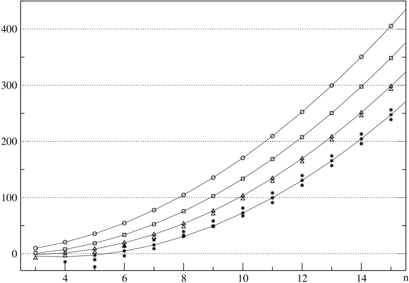
Figure 1: The eigenvalues of the matrices $\widetilde{\Delta}$. The circles correspond to the leading branch $\lambda_{0}$ from (5.3), the squares, triangles and asterisks correspond to the branches $\lambda_{1}$, $\lambda_{2*}$ and $\lambda_{3*}$ from (5.4).

It is interesting to note that, for $n=1$, the only eigenvalue $\lambda(1)=0$ (which is known exactly) belongs to neither curve. Probably this fact is related to the observation that the agreement between the formulae (5.3), (5.4) and the exact numerical values for the eigenvalues improves if the correction term is written in the form $O(1/(n-1))$.

In their turn, the expressions (5.3), (5.4) demonstrate interesting regularities: the leading (quadratic in $n$) term is the same for all the branches; the next-to leading term (linear in $n$) is negative with the odd coefficient growing with the step of 4. The branches can be grouped according the value of that coefficient, and the number of branches with a given value grows: there is one branch in the first two groups, two branches in the third group, three branches in the fourth group etc. It is also worth noting that if the constant (independent of $n$) terms in (5.3) are replaced with the closest integer numbers and the $O(1/n)$ corrections are neglected, the resulting expressions give exactly the integer parts for all the eigenvalues.

These regularities are also illustrated by figure 1, where all the positive eigenvalues of the matrices $\widetilde{\Delta}$ are shown with $n$ from 3 to 15; according to (4.5), they correspond to “dangerous” composite operators with negative critical dimensions. The solid lines correspond to representatives of the principal branches: $\lambda_{0}$ from (5.3) and $\lambda_{1}$, $\lambda_{2,1}$, $\lambda_{3,3}$ from (5.4). They are plotted according the formulae (5.3) and (5.4) neglecting the $O(1/n)$ corrections. The other branches from the groups $\lambda_{2,*}$ and $\lambda_{3,*}$ are not shown by solid lines in order to make the picture more graspable. The circles denote the maximal eigenvalues of the matrices $\widetilde{\Delta}$, and the squares denote the next-to-maximal ones; they lie exactly on the principal branches $\lambda_{0}$ and $\lambda_{1}$ from (5.3), (5.4). The eigenvalues that correspond to the two branches of the group $\lambda_{2,*}$ are denoted by triangles and the eigenvalues of the three branches of the next group $\lambda_{3,*}$ are denoted by asterisks.

The general formulae (5.3), (5.4) for negative eigenvalues do not work so well in comparison with positive ones. This fact is illustrated by the same figure 1, where some negative eigenvalues (with $n$ from 4 to 6) are also shown. It turns out, however, that the negative eigenvalues form their own pronounced branches; the principal one is described by the empiric formula

$$\lambda_{0}^{(-)}(n)=-n^{2}+2+O(1/n).$$ (5.5)

Comparison of expressions (5.3) and (5.5) shows that the ratio of the maximal positive and maximal (by modulus) negative eigenvalues of the matrix $\widetilde{\Delta}$ tends to 2 as $n$ grows, in agreement with the numerical values for $24\leq n\leq 28$ given in (5.2).

6 Conclusion

By means of the field theoretic renormalization group and operator product expansion we studied the problem of anomalous scaling of the transverse vector field passively advected by a turbulent velocity field. The dynamics of the vector field is governed by the stochastic equation (1.3), (1.4), while the velocity was described by the stirred NS equation (1.6), (1.7), (1.8). The anomalous scaling arises as a consequence of the existence in the OPE of the so-called “dangerous” composite fields (operators) with negative critical dimensions. The leading terms of the inertial-range asymptotic behaviour of the structure functions (3.1), (3.2) are determined by the matrices of critical dimensions of the families of composite fields of the form $(\partial\theta\partial\theta)^{2n}$. For $d\to\infty$, dangerous operators can be present only in the subsets of operators of the special form, (4.1), (4.2), and the corresponding matrices of critical dimensions can be constructed by means of a simple algorithm. This allowed us to calculate them in the leading order of the double expansion in $y$ and $1/d$ up to the order $n=28$. The eigenvalues of those matrices (that is, the critical dimensions of the corresponding families of operators) demonstrate intriguing pronounced regularities. This fact allows one to describe them by simple empiric formulae which become practically exact as $n$ grows. In particular, the leading term of the asymptotic behaviour of the structure function (3.1) in the inertial range has the form

$$S_{2n}({\bf r})\simeq D_{0}^{-n}\,r^{n(2-y/3)}\,(mr)^{\Delta_{n}},$$

$$\Delta_{n}=-(y/3d)\left(2n^{2}-3n+1/2+O(1/n)\right),$$ (6.1)

there are also explicit expressions for the correction exponents. Thus, the complete description of the anomalous scaling for our vector model is given for all $n$.

The regularities demonstrated by the critical dimensions of the sets of composite fields and their branches, discussed in the present paper, are so intriguing that we cannot but think that some unknown symmetry lies behind them. One may think that understanding the relation between the anomalous scaling, statistical conservation laws and operator product expansion will be useful here; see [29] for the scalar Kraichnan’s case. In this connection it is interesting to note that the critical dimensions of certain composite operators in quantum chromodynamics (QCD) and in the $N=4$ supersymmetric gauge theories also show interesting behaviour (also in the large-$n$ limit and in the one-loop approximation): in particular, for the QCD case the corresponding evolution equations appear equivalent to the integrable Heisenberg model [30].

The Kraichnan’s rapid-change model of passive scalar advection is sometimes referred to as “the Ising model of fluid turbulence.” In this connection, it is worth recalling that the original Ising (or, better to say, Lentz–Ising) model of magnetism, first introduced in 1920 [31], has still remained a source of inspiration for new physical and mathematical ideas and techniques like integrability, fermion–boson transformations, conformal invariance and discrete holomorphisity: for a recent discussion, see [32] and references therein.

One may think that, in spite of a great deal of work devoted to Kraichnan’s model and its descendants, the deep physical and mathematical contents that lie behind them are not completely disclosed. We believe that identifying the hypothetical symmetry of the passive vector problem that gives rise to the intriguing regularities discussed in the present paper will help to reach a deeper understanding of the anomalous scaling in the real fluid turbulence.

References

References

- [1] Falkovich G, Gawȩdzki K and Vergassola M 2001 Rev. Mod. Phys. 73 913
- [2] Frisch U 1995 Turbulence: The Legacy of A N Kolmogorov (Cambridge: Cambridge University Press)
-
[3]
Gawȩdzki K and Kupiainen A 1995 Phys. Rev. Lett. 75 3834
Bernard D, Gawȩdzki K and Kupiainen A 1996 Phys. Rev. E54 2564 -
[4]
Chertkov M, Falkovich G, Kolokolov I and Lebedev V 1995
Phys. Rev. E52 4924
Chertkov M and Falkovich G 1996 Phys. Rev. Lett. 76 2706 - [5] Adzhemyan L Ts, Antonov N V and Vasil’ev A N 1998 Phys. Rev. E58 1823
- [6] Antonov N V 2006 J. Phys. A: Math. Gen. 39 7825
- [7] Adzhemyan L Ts, Antonov N V, Barinov V A, Kabrits Yu S and Vasil’ev A N 2001 Phys. Rev. E63 025303(R), Phys. Rev. E64 019901(E), Phys. Rev. E 64 056306
- [8] Adzhemyan L Ts and Runov A V 2001 Vestnik SPbU, Ser. 4: Phys. Chem. 4 85
- [9] Arad I and Procaccia I 2001 Phys. Rev. E63 056302
- [10] Adzhemyan L Ts, Antonov N V and Runov A V 2001 Phys. Rev. E64 046310
- [11] Adzhemyan L Ts, Antonov N V, Gol’din P B and Kompaniets M V 2009 Vestnik SPbU, Ser. 4: Phys. Chem. 1 56
-
[12]
Novikov S V
2002 Vestnik SPbU, Ser. 4: Phys. Chem. 4 77;
2003 Theor. Math. Phys. 136 936;
2006 J. Phys. A: Math. Gen. 39 8133
Adzhemyan L Ts and Novikov S V 2006 Theor. Math. Phys. 146 393 - [13] Jurčišinova E, Jurčišin M, Remecký R and Scholtz M 2008 Phys. Particles Nuclei Lett. 5 219
-
[14]
Adzhemyan L Ts, Antonov N V, Mazzino A,
Muratore-Ginanneschi P and Runov A V 2001 Europhys. Lett. 55
801
Antonov N V, Hnatich M, Honkonen J and Jurčišin M 2003 Phys. Rev. E68 046306
Arponen H 2009 Phys. Rev. E79 056303
Antonov N V and Gulitskiy N M 2012 arXiv:1212.4141[cond-mat.stat-mech]; to be published in Theor. Math. Phys. -
[15]
Vergassola M 1996 Phys. Rev. E53 R3021
Rogachevskii I and Kleeorin N 1997 Phys. Rev E56 417
Lanotte A and Mazzino A 1999 Phys. Rev. E60 R3483
Arad I, Biferale L and Procaccia I 2000 Phys. Rev. E61 2654
Antonov N V, Lanotte A and Mazzino A 2000 Phys. Rev. E61 6586
Hnatich M, Jurčišin M, Mazzino A and Šprinc S Acta Phys. Slovaca 2002 52 559
Hnatich M, Honkonen J, Jurčišin M, Mazzino A and Šprinc S 2005 Phys. Rev. E71 066312
Jurčišinova E, Jurčišin M and Remecký R 2009 J. Phys. A: Math. Theor. 42 275501
Antonov N V and Gulitskiy N M 2012 Lecture Notes in Comp. Science 7125/2012 128
Antonov N V and Gulitskiy N M 2012 Phys. Rev. E85 065301(R)
Jurčišinova E and Jurčišin M 2012 J. Phys. A: Math. Theor. 45 485501 -
[16]
De Dominicis C and Martin P C 1979 Phys. Rev. A 19 419
Sulem P L, Fournier J D and Frisch U 1979 Lecture Notes in Physics 104 321
Fournier J D and Frisch U 1983 Phys. Rev. A 28 1000
Adzhemyan L Ts, Vasil’ev A N and Pis’mak Yu M 1983 Theor. Math. Phys. 57 1131 -
[17]
Adzhemyan L Ts, Antonov N V and Vasil’ev A N 1996
Uspekhi Fiz. Nauk 166 1257 [In Russian; English translation:
1996 Phys. Usp. 39 1193]
Adzhemyan L Ts, Antonov N V and Vasiliev A N 1999 The Field Theoretic Renormalization Group in Fully Developed Turbulence (Gordon & Breach, London) - [18] Vasil’ev A N 2004 The Field Theoretic Renormalization Group in Critical Behavior Theory and Stochastic Dynamics (Boca Raton: Chapman & Hall/CRC)
-
[19]
Adzhemyan L Ts, Antonov N V and Kim T L 1994
Theor. Math. Phys. 100 1086
Antonov N V, Borisenok S V and Girina V I 1996 Theor. Math. Phys. 106 75
Antonov N V and Vasil’ev A N 1997 Theor. Math. Phys. 110 97 - [20] Kraichnan R H 1974 J. Fluid. Mech. 64 737
- [21] Fournier J-D, Frisch U, Rose H A 1978 J. Phys. A: Math. Gen. 11 187
- [22] Yakhot V 1998 E-print LANL chao-dyn/9805027
- [23] Frisch H L, Schultz M 1994 Physica A: Stat. Theor. Phys. 211 37
- [24] Runov A V 1999 E-print LANL chao-dyn/9906026
- [25] Adzhemyan L Ts, Antonov N V, Gol’din P B, Kim T L and Kompaniets M V 2008 J. Phys. A: Math. Gen. 41 495002; 2009 Vestnik SPbU, Ser. 4: Phys. Chem. 4 238; 2009 Theor. Math. Phys. 158 391
- [26] Adzhemyan L Ts, Antonov N V, Kompaniets M V and Vasil’ev A N 2003 Int. J. Mod. Phys. B 17 2137
- [27] Adzhemyan L Ts, Vasil’ev A N and Hnatich M 1984 Theor. Math. Phys. 58 47
- [28] Adzhemyan L Ts, Antonov N V, Honkonen J and Kim T L 2005 Phys. Rev. E 71 016303
-
[29]
Kupiainen A and Muratore-Ginanneschi P 2007
J. Stat. Phys. 126 669
Mazzino A and Muratore-Ginanneschi P 2009 Phys. Rev. E80 025301
Muratore-Ginanneschi P 2012 Physica D241 276 -
[30]
Braun V M, Derkachov S E and Manashov A N 1998 Phys. Rev. Lett.
81 2020
Belitsky A V, Derkachov S E, Korchemsky G P and Manashov A N 2004 Phys. Lett. B594 385
Derkachov S E and Manashov A N 2010 J. Math. Sci. 168 837 -
[31]
Lentz W 1920 Z. Phys. 21 613
Ising E 1925 Z. Phys. 31 253
Brush S G 1967 Rev. Mod. Phys. 39 883 - [32] International Meeting “Conformal Invariance, Discrete Holomorphicity and Integrability” (Helsinki, 10–16 June 2012). Organizers Antti Kemppainen and Kalle Kytölä, Web page: https://wiki.helsinki.fi/display/mathphys/cidhi2012