Proportional Paths, Barodesy, and
Granular Solid Hydrodynamics

Abstract

Propotional paths as summed up by the Goldscheider Rule (gr) – stating that given a constant strain rate, the evolution of the stress maintains the ratios of its components – is a characteristics of elasto-plastic motion in granular media. Barodesy, a constitutive relation proposed recently by Kolymbas, is a model that, with gr as input, successfully accounts for data from soil mechanical experiments. Granular solid hydrodynamics (gsh), a theory derived from general principles of physics and two assumptions about the basic behavior of granular media, is constructed to qualitatively account for a wide range of observation – from elastic waves over elasto-plastic motion to rapid dense flow. In this paper, showing the close resemblance of results from Barodesy and gsh, we further validate gsh and provide an understanding for gr.

I Introduction

One focus of soil mechanical experiments is the stress evolution $\sigma_{ij}\left(t\right)$ for given strain rate $v_{ij}\equiv\frac{1}{2}(\nabla_{i}v_{j}+\nabla_{j}v_{i})$ and density $\rho$ gudehus2010 . Three striking characteristics being observed at slow, elasto-plastic rates are (1) rate-independence, (2) the existence of a critical state wood1990 , and (3) proportional paths as summed up by the Goldscheider Rule (gr) goldscheider . Rate-independence means that if the given strain rate $v_{ij}$ is a constant, the stress $\sigma_{ij}(t)$ is a function of the strain $\varepsilon_{ij}\equiv\int v_{ij}{\rm d}t=v_{ij}t$, and does not depend on the actual rate.

The critical state is an expression of “ideal plasticity.” Starting from an isotropic stress $\sigma_{ij}=P\delta_{ij}$, and applying a constant shear rate $v_{ij}^{*}$ (^∗ denotes the traceless part) – while maintaining a vanishing trace $v_{\ell\ell}=0$ to keep the density $\rho$ constant – a granular system will always go into an asymptotic, stationary state, in which the stress $\sigma^{c}_{ij}$ no longer changes with time, although $v_{ij}$ goes on providing a constant rate of deformation. We shall call this asymptotic state – characterized by the direction of the rate $v_{ij}^{*}/v_{s}$ (where $v_{s}^{2}=v_{ij}^{*}v_{ij}^{*}$) and the density $\rho$ – the critical state. (The asymptotic state is more typically arrived at for given shear rate $v_{ij}^{*}$, at constant pressure $P\equiv\frac{1}{3}\sigma_{\ell\ell}$ or one of the principle stress value $\sigma_{11}$, rather than the density. And there are some in the engineering community who insist on restricting the term critical state to the results of this second type of approaches. The narrower definition would be sensible if the respective asymptotic states were different. We do not believe this to be the case, for rather basic reasons, as will become clear in section II.)

The Goldscheider Rule or gr is a generalization of the critical state. First, it states that a granular system will converge onto the same critical state associated with $v_{ij}^{*}/v_{s}$ and $\rho$, starting from any initial stress, not only an isotropic one. And second, it postulates the existence of asymptotic states also for cases of changing $\rho$ – a point that we believe may be understood as follows: In the principal strain axes $(\varepsilon_{11},\varepsilon_{22},\varepsilon_{33})$, a constant $v_{ij}^{*}$ means the system moves with a constant rate along its direction, $\varepsilon_{11}/\varepsilon_{22}=v_{11}^{*}/v_{22}^{*}$, $\varepsilon_{22}/\varepsilon_{33}=v_{22}^{*}/v_{33}^{*}$. This circumstance is referred to as a proportional strain path. In the stress space, $\sigma^{c}_{ij}$ is a stationary dot and does not move. Now, adding a constant $v_{\ell\ell}$ to the isochoric strain path, $[v_{ij}^{*}+\frac{1}{3}v_{\ell\ell}\delta_{ij}]\,t$, we need to keep $v_{\ell\ell}$ small compared to $v_{s}$, such that an initial stress has sufficient time to converge without breaching the random closest or loosest packing – the grains get crushed in the first case, and loose contacts with one another in the second. Then one expects the asymptotic state to be approximately given by the critical stress $\sigma^{c}_{ij}(\rho)$ associated with the same isochoric strain path $v_{ij}^{*}\,t$. As time passes, the density $\rho$ will change, so will the critical state $\sigma^{c}_{ij}(\rho)$. But it will remain associated with $v_{ij}^{*}\,t$. Interestingly, gr states that this stress path is also proportional, meaning $\sigma_{11}(t)/\sigma_{22}(t)$, $\sigma_{22}(t)/\sigma_{33}(t)$ also remain constant.

The statements of gr as rendered by Kolymbas barodesy are: (1) Proportional strain paths starting from the stress $\sigma_{ij}=0$ are associated with proportional stress paths. (2) Proportional strain paths starting from $\sigma_{ij}\not=0$ lead asymptotically to the corresponding proportional stress paths obtained when starting at $\sigma_{ij}=0$. (A caveat: Although Goldscheider is a prudent and reliable experimenter, his data base is rather small goldscheider .) The initial value $\sigma_{ij}=0$ is a mathematical idealization, neither easily realized nor part of the empirical data that went into gr. So we take its core statement as: Applying a proportional strain path, there is an asymptotic line to which all other stresses converge. This stress path is also proportional, such that proportional strain and stress paths form pairs.

Barodesy barodesy is a recent, impressively realistic constitutive model by Kolymbas, the originator of hypoplasticity kolymbas1 . His purpose is to further improve the quantitative account of granular media’s motion, and to reduce the considerable liberty when constructing hypoplastic models. He did this by starting explicitly from gr. In the present paper, we take Barodesy (as specified below, in Sec III), as a constitutive equation with a reduced set of variables, which reflects highly condensed and intelligently organized empirical data, to which the results of gsh are compared.

gsh is a theory of continuum mechanics derived from two notions that we hold to be the basic physics of granular media granR2 . When constructing the theory employing general principles, we had little experimental data in mind, and certainly never needed to choose a subset of these. Therefore, if not totally wrong, gsh should be adequate and correct in a broad-ranged fashion. Until now, gsh has shown itself capable of accounting for phenomena as diverse as static stress distribution ge-1 ; ge-2 ; granR1 , incremental stress-strain relation SoilMech , yield JL2 ; 3inv , propagation and damping of elastic waves ge4 , elasto-plastic motion JL3 , the critical state critState , shear band and fast dense flow denseFlow . Comparison to Barodesy is a further hard test for gsh, especially because any agreement could not possibly have been planned for. Moreover, gsh provides an understanding for gr, and embeds it among the many granular phenomena already understood within the framework of gsh.

Finally, we amplify on the point why comparing gsh successfully to Barodesy validates the former. First, we note the qualitative difference between a physicist’s theory and an engineering one, which are in fact constructs of different raison d’être: Physicists aim to first of all gain a qualitative understanding of a given system, while engineers want primarily to organize and mathematically condense experimental data gained in that system. When constructing a theory, physicists typically start from some notions about the basic behavior of a system, calling them motivation. If broadly validated, physicists will conclude these notions are right, considering this a gain in understanding. Two theories with different notions will contradict each other eventually, even if they initially agree with respect to some experiments. Two engineering theories may look very different mathematically, but if essentially the same set of data was used in constructing these theories, they will not contradict each other starkly – though small deviations will generally exist. An agreement between gsh and Barodesy, showing that a theory deduced from some notions, hence quite possibly wildly off the mark, produces results that are seen in experiments, is therefore indeed a validation. On the other hand, there are always shades of gray – engineers with a fundamentalist’s heart and physicists with a most pragmatic mindset. But all will agree that a mature theory should be both realistic and derived from the specific physics of the system under focus.

We shall in future compare gsh to more constitutive models and experiments on elasto-plastic motion. Recent experiments include uniaxial tests aaa10 , the settlement aaa8 , and systematic triaxial measurements aaa2 , though we do not expect either models or experiments to deviate strongly from Barodesy or each other, for the reasons mentioned above. A recent paper aaa1 stands out, because it connects the constitutive model to particle-level properties. Generally speaking, one needs to heed the cautionary words by Schwedes aaa11 , that these setups are typically designed for engineering purpose, and the data may depend on operational details (such as skill of the experimenters and their level of training). So care has to be taken when adopting their data. A major difficulty, we believe, comes from the influence of the initial state, from the lack of information on boundary conditions, and from the presence of water (that gsh not yet considers).

DEM simulations are nowadays a popular approach employed by both physicists and engineers, see eg. aaa5 ; aaa6 ; aaa7 ; aaa9 ; aaa12 ; aaa13 ; aaa14 ; aaa15 ; aaa16 ; aaa17 ; aaa18 . The best are often qualitatively perfect, but numerically different from experimental results. Therefore, a comparison to gsh requires us to treat them as different systems, with their own values for energy and transport coefficients. Unfortunately, the associated calibration process is time-consuming and laborious.

II The Equations of GSH

II.1 Two-Stage Irreversibility

The essence of granular physics, we contend, is encapsulated by two notions: two-stage irreversibility and variable transient elasticity. The first is related to the three spatial scales of any granular media: (a) the macroscopic, (b) the intergranular, and (c) the inner granular. Dividing all degrees of freedom into these three categories, we treat those of (a) differently from (b,c). Macroscopic degrees of freedom, such as the slowly varying stress or velocity fields, are specified and employed as explicit state variables, but intergranular and inner granular degrees are treated summarily: Instead of being specified, only their contribution to the energy is considered and taken, respectively, as granular and true heat. So we do not account for the motion of a jiggling grain, only include its strongly fluctuating kinetic and elastic energy as contributions to the granular heat $\int T_{g}{\rm d}s_{g}$, characterized by the granular entropy $s_{g}$ and temperature $T_{g}$. Similarly, a phonon, or any elastic vibration within the grain, are taken as part of true heat, $\int T{\rm d}s$. Clearly, there are only a handful of macroscopic degrees of freedom (a), innumerable intergranular ones (b), and yet many orders of magnitude more inner granular ones (c). So the statistical tendency to equally distribute the energy among all degrees of freedom implies that the energy decays from (a) to (b,c), and from (b) to (c), never backwards. This is what we call two-stage irreversibility.

Accounting for higher densities, when enduring contacts abound and granular jiggling is small, we expand $w_{T}$ to obtain $w_{T}=s_{g}^{2}/2b$, with $T_{g}\equiv\partial w_{T}/\partial s_{g}=s_{g}/b$ and $w_{T}\sim T_{g}^{2}$. There is no linear term because $s_{g},T_{g}=0$ is an energy minimum. (The usual granular temperature $T_{G}$, defined as 2/3 of a grain’s average kinetic energy, is useful only in the dilute limit, when the fluctuating elastic energy may be neglected, and $w_{T}\sim T_{G}\sim T_{g}^{2}$.) Neglecting nonuniform situations, the balance equation for $s_{g}$ reads

$$T_{g}{\partial_{t}s_{g}}=\eta_{g}v_{s}^{2}+\xi_{g}v_{\ell\ell}^{2}-\gamma T_{g}^{2},$$ (1)

with $v_{s}^{2}\equiv v_{ij}^{\ast}v_{ij}^{\ast}$, and $v_{ij}^{\ast}$ the traceless part of $v_{ij}$. Also: $\partial_{t}\equiv\frac{\partial}{\partial_{t}}$. The first two term on the right side accounts for viscous heating, the third for the leak of granular heat from (b) to (c). The viscosities $\eta_{g},\xi_{g}$ and the relaxation rate $\gamma$ are parameters of gsh and functions especially of $T_{g},\,\rho$. We take granR2

$$T_{g}=s_{g}/(\rho b),\quad\eta_{g}=\eta_{1}T_{g},\quad\gamma=\gamma_{0}+\gamma_{1}T_{g},$$ (2)

noting that for what we call the hypoplastic regime of slightly elevated $T_{g}$, in which hypoplasticity and Barodesy hold, $\gamma_{0}\ll\gamma_{1}T_{g}$ may be neglected. And we neglect $\xi_{g}v_{\ell\ell}^{2}$, because $\eta_{g}v_{s}^{2}\gg\xi_{g}v_{\ell\ell}^{2}$ in all typical experiments. For constant shear rate $v_{ij}^{\ast}$, Eq (1) is a relaxation equation, with $T_{g}$ quickly settling into its stationary value,

$$T_{g}=\sqrt{\eta_{1}/\gamma_{1}}\,v_{s}.$$ (3)

It is then no longer independent. The coefficients $1/b,\eta_{1},\gamma_{1}$ are functions of $\rho$,

$$b\sim(\rho_{cp}-\rho)^{0.1},\quad\gamma_{1},\,\eta_{1}\sim(\rho_{cp}-\rho)^{-1},$$ (4)

where $\rho_{cp}$ is the closest packed density. We stand behind the $T_{g}-$dependence with much more confidence than that of the density, for two reasons: First, there are no comparably general arguments to extract the $\rho$ dependence. Second, probably because of this, the observed dependence is not universal. The above dependence fits glass beads data, while $\gamma_{1}\sim(\rho_{cp}-\rho)^{-0.5}$, $\eta_{1}\sim(\rho_{cp}-\rho)^{-1.5}$ seem more suitable for polystyrene beads, see denseFlow .

II.2 Variable Transient Elasticity

Our second notion, variable transient elasticity, addresses granular elasticity and plasticity. The free surface of a granular system at rest can be inclined, or tilted. When perturbed, when the grains jiggle and $T_{g}\not=0$, the inclination will be reduced until the surface is horizontal. The stronger the grains jiggle, the faster this process is. We take this as indicative of a system that is elastic for $T_{g}=0$, turning transiently elastic for $T_{g}\not=0$, with a stress relaxation rate that grows with $T_{g}$. A relaxing stress is typical of any viscous-elastic system such as polymers. The unique circumstance here is that the relaxation rate is not a material constant, but a function of the state variable $T_{g}$. As we shall see, it is this dynamically controlled, variable transient elasticity – a simple fact at heart – that underlies the complex behavior of granular plasticity. Realizing it yields a most economic way to capture granular rheology.

Employing a strain field rather than the stress as a state variable usually yields a simpler description, because the former is in essence a geometric quantity, while the latter contains material parameters such as stiffness. Yet one cannot use the standard strain field $\varepsilon_{ij}$ as a granular state variable, because the relation between stress and $\varepsilon_{ij}$ lacks uniqueness when the system is plastic. A number of engineering theories divide the strain into two fields, elastic and plastic, $\varepsilon_{ij}=u_{ij}+\varepsilon^{(p)}_{ij}$, with the first accounting for the reversible and second for the irreversible part. They then employ $\varepsilon_{ij}$ and $\varepsilon^{(p)}_{ij}$ as two independent strain fields to account for granular plasticity Houlsby .

We believe that one should, on the contrary, take the elastic strain $u_{ij}$ as the sole state variable, as there is a unique relation between $u_{ij}$ and the elastic stress $\sigma_{ij}$ – if both are related via the elastic energy: Shearing a granular system, part of the strain goes into deforming the grains, changing their elastic energy. The rest is spent sliding and rolling the grains. Taking $u_{ij}$ as the portion that changes the energy and deforms the grains, the elastic energy $w(u_{ij})$ is by definition a function of $u_{ij}$ alone. And since an elastic stress $\sigma_{ij}(u_{ij})$ only exists when the grains are deformed, it is also a function of $u_{ij}$. Therefore, we employ $u_{ij}$ as the sole state variable, and discard both $\varepsilon_{ij}$ and $\varepsilon^{(p)}_{ij}$. Doing so preserves many useful features of elasticity, especially the (so-called hyper-elastic) relation,

$$\sigma_{ij}=-\partial w(u_{ij},\rho)/\partial u_{ij}|_{\rho}.$$ (5)

This is derived in granR2 but easy to understand via an analogy. Driving up a snowy hill slowly, the car wheels will grip the ground part of the time, slipping otherwise. (We assume a slowly turning wheel and quickly changing, intermittent stick-slip behavior.) When the wheels do grip, the car moves upward and its gravitational energy $w^{grav}$ is increased. If we divide the wheel’s rotation into a gripping (e) and a slipping (p) portion, $\theta=\theta^{(e)}+\theta^{(p)}$, we know we may ignore $\theta^{(p)}$, and compute the torque on the wheel as $\partial w^{grav}/\partial\theta^{(e)}$, same as Eq.(5). How much the wheel turns or slips, how large $\theta$ or $\theta^{(p)}$ are, is irrelevant for the torque.

The functional dependence of the energy density $w(u_{ij})$ is an input in gsh, as it cannot be obtained from general principles. The one we propose, because we find it both simple and appropriate, is specified below, in Sec II.4. Once it is given, so is the elastic stress, for which there is therefore an explicit expression, in terms of the state variables $u_{ij}$ and $\rho$.

The evolution equation for $u_{ij}$, as derived in granR2 , may be divided into that of the trace $\Delta\equiv-u_{\ell\ell}$ and the traceless part $u_{ij}^{\ast}$,

$${\partial_{t}u_{ij}^{\ast}} = \left(1-\alpha\right)v_{ij}^{\ast}-\lambda T_{g}u_{ij}^{\ast},$$ (6)

$${\partial_{t}\Delta} = (1-\alpha)v_{\ell\ell}+\alpha_{1}u_{lk}^{\ast}v_{lk}^{\ast}-\lambda_{1}T_{g}\Delta.$$ (7)

Comparing them to the fully elastic equation, ${\partial_{t}u_{ij}}=v_{ij}$, we realize $\alpha$ is a gear shift factor, as a higher rate is necessary to achieve the same deformation; while $\alpha_{1}$ is a dilatancy factor, accounting for the granular phenomenon that a shear flow leads to compression or decompression. Both $\alpha$ and $\alpha_{1}$ are off-diagonal Onsager coefficients that depend on $T_{g}$, though we may take them as constant in the present context.

The two terms $\sim T_{g}$ are relaxation terms, accounting for the loss of deformation $\Delta,u_{ij}^{\ast}$ (and the associated loss of the stress) when $T_{g}$ is finite. The relaxation rate grows with $T_{g}$, and is typically about 3 times as large for $u_{ij}^{\ast}$ as $\Delta$, hence $\lambda\approx 3\lambda_{1}$ JL3 . This is how variable transient elasticity is mathematically encoded. Replacing $T_{g}$ with the shear rate $v_{s}$ for the stationary case of Eq.(3), we find the above two equations explicitly rate independent. Denoting $\lambda T_{g}=\lambda\sqrt{\eta_{1}/\gamma_{1}}v_{s}\equiv\Lambda v_{s}$, $\lambda_{1}T_{g}\equiv\Lambda_{1}v_{s}$, we take, as tentatively as before,

$$\Lambda,\,\Lambda_{1},\,\alpha,\,\alpha_{1}\sim\rho_{cp}-\rho,$$ (8)

assuming that the plastic phenomena of relaxation, softening and dilatancy are no longer operative at $\rho=\rho_{cp}$. For a given shear rate $v_{ij}$, Eqs (6,7) are relaxation equations. Denoting $u_{s}^{2}=u_{ij}^{\ast}u_{ij}^{\ast}$, $v_{s}^{2}=v_{ij}^{\ast}v_{ij}^{\ast}$, the system will converge onto the rate independent asymptotic value (denoted by a superscript ^c) of

$$u^{c}_{s}=\frac{1-\alpha}{\Lambda},\quad\frac{\Delta^{c}}{u^{c}_{s}}=\frac{\alpha_{1}}{\Lambda_{1}}+\frac{1-\alpha}{u^{c}_{s}\Lambda_{1}}\frac{v_{\ell\ell}}{v_{s}},$$ (9)

and $u_{ij}^{\ast}|^{c}=v_{ij}^{\ast}(u^{c}_{s}/v_{s})$ implying $u_{ij}|^{c}$ and $v_{ij}$ have the same orientation and principal axes. Note also for ${v_{\ell\ell}}\ll{v_{s}}$, the density dependence of ${\Delta^{c}}/{u^{c}_{s}}\approx{\alpha_{1}}/{\Lambda_{1}}$ cancels.

Given the elastic strain $u_{ij}|^{c}=u_{ij}^{*}|^{c}-\frac{1}{3}\Delta^{c}\delta_{ij}$ and the density $\rho$, the elastic stress is also given. For $v_{\ell\ell}=0$, this is simply the ideally plastic, stationary, critical state. The elastic strain and the associated stress do not change with time, because the deformation rate and the relaxation cancel, $\partial_{t}u_{ij}\sim\partial_{t}\sigma_{ij}=0$. Calculating an approach to this state, starting from an isotropic stress and keeping the $\sigma_{1}$ constant, the resultant curves for $q\equiv\sigma_{3}-\sigma_{1}=\sigma_{s}\sqrt{3/2}$ and the void ratio $e\equiv\rho_{g}/\rho-1$ ($\rho_{g}$: grain’s density), against the strain $\varepsilon_{3}$ in triaxial tests (cylinder axis along 3), resemble a textbook illustration of the critical state, see Fig 1.

Figure 1: Seemingly a textbook illustration of the critical state, this is the result of a gsh calculation: Shear stress $q$ and void ratio $e$ against the strain $\varepsilon_{3}$ in triaxial tests (cylinder axis along 3), at given $\sigma_{1}$ and strain rate $\varepsilon_{3}/t$, for an initially dense ($\rho_{0}=0.97\rho_{cp}$) and loose ($\rho_{0}=0.95\rho_{cp}$) sample. Insets are critical stress $q^{c}$ and density $\rho^{c}$ against $\sigma_{1}$; with $B_{0}=7$GPa, ${\cal A}=0.6{\cal B}$, $\rho_{\ell p}=0.85\rho_{cp}$, $\alpha_{1}=750(1-\rho/\rho_{cp})$, $\alpha=0.7$, $\Lambda=2850(1-\rho/\rho_{cp})$, $\Lambda/\Lambda_{1}=3.3$, and in SI units: $\gamma_{1}=6\cdot 10^{5}$, $\eta_{1}=0.15$ (ie. $\Lambda=114$, $\alpha_{1}=30$ for $\rho=0.96\rho_{cp}$, as in JL3 ).

For $v_{\ell\ell}/v_{s}$ finite but small, neither the direction nor the magnitude of $u_{ij}$ and $\sigma_{ij}$ change much, as conjectured in the introduction, though the mean stress will grow or decrease with the density. To see how it changes, and why it follows a proportional path, we need the explicit expression for the stress, specified in the next section, Sec II.4. But we can already see the reason for gr’s second statement: Starting from any initial value $u_{ij}\not=u_{ij}|^{c}$, the deviation $u_{ij}-u_{ij}|^{c}$ will, according to Eqs.(6) and (7), vanish exponentially. Clearly, variable transient elasticity is what lies behind both the critical state and gr.

Finally, we note that the Cauchy stress, or total stress, $\sigma_{ij}^{tot}$ is softer than the elastic one,

$$\sigma_{ij}^{tot}=(1-\alpha)\sigma_{ij},$$ (10)

with the same factor as in Eqs.(6) or (7). This is a result of the Onsager reciprocity relation LL5 , but it may less formally also be seen as the flip side of the gear shift factor: when a higher rate is needed to achieve a certain elastic deformation, energy conservation requires the restoring force to be smaller by the same factor.

For very high rates – such as present in heap flow or avalanches, the seismic pressure $P_{T}\sim T_{g}^{2}\sim v_{s}^{2}$ resulting from violent jiggling of the grains, and the viscous stress, $\eta_{g}v_{ij}^{*}=\eta_{1}T_{g}v_{ij}^{*}$, again of shear rate squared, become relevant and destroy the rate independence. We neglect both in this paper – though not the viscous granular heating of Eq.(3).

II.3 Yield versus the Critical State

In a space spanned by stress components and density, there is a surface that divides two regions in any granular media, one in which the grains necessarily move, another in which they may be at rest. This surface may be referred to as the yield surface. Equivalently, we may take the yield surface as the divide between two regions, one in which elastic solutions are stable, and another in which they are not – clearly, the medium may be at rest for a given stress only if an appropriate elastic solution is stable. Since the elastic energy of any solution satisfying force equilibrium $\nabla_{j}\sigma_{ij}=0$ is an extremum granR2 , the energy is convex and minimal in the stable region, concave and maximal in the unstable one —in which infinitesimal perturbations suffice to destroy the state of rest.

Yield is clearly a completely distinct concept from the critical state as discussed above – one a static phenomenon, the other dynamic. The first is a convexity transition of the elastic energy, to be probed by quasi-static motion at vanishing $T_{g}$, say by slowly tilting a plate with a layer of grains. The second is a stationary solution of the relaxation equation for the elastic strain $u_{ij}$ at given shear rate, and relevantly, at an elevated $T_{g}$. It is comparable to the stationary solution of any diffusion equation. The yield and critical shear stresses are frequently similar in magnitude, but the yield stress needs to be larger than the highest shear stress achieved during the approach to the critical state. Otherwise, the system will abandon the approach and develop shear bands instead, see Fig.2 below.

Many believe that the approach to the critical state is accomplished at low enough shear rates to be considered quasi-static. We contend that a quasi-static motion is one that visits a series of static, equilibrium states, with $T_{g}\to 0$. The rate of dissipation must be negligibly small. The rate-independent, hypoplastic motion taking place during an approach to the critical state maintains an elevated $T_{g}$ that allows irreversible, dissipative relaxation of the elastic strain. In the critical state, this dissipative process, having the same magnitude as the reactive (ie. elastic) deformation rate, certainly cannot be neglected.

II.4 Granular Elastic Energy

The elastic energy density $w$ is a function of the three independent strain invariants, $\Delta,u_{s}$ and $u_{t}\equiv\sqrt[3]{u_{ik}^{\ast}u_{kj}^{\ast}u_{ji}^{\ast}}$. For granular materials, the following expression is appropriate in many respects,

$$w={\cal B}\sqrt{\Delta}\left(\frac{2}{5}\Delta^{2}+\frac{1}{\xi}u_{s}^{2}-\frac{\chi}{\xi}\frac{u_{t}^{3}}{\Delta}\right),$$ (11)

and was instrumental in achieving the agreements with all the granular phenomena mentioned above, especially static stress distribution, incremental stress-strain relation, and elastic waves. Varying the coefficient $\chi$, the yield surface changes to resemble different yield laws, including Drucker-Prager, Lade-Duncan, Coulomb, and Matsuoka-Nakai, see 3inv . For qualitative considerations, however, it is frequently sufficient to set $\chi=0$. We then find the elastic energy convex only for

$$u_{s}/\Delta\leq\sqrt{2\xi},\quad\text{or}\quad\sigma_{s}/P\leq\sqrt{2/\xi},$$ (12)

where $P\equiv\sigma_{kk}/3$, $\sigma_{s}\equiv\sqrt{\sigma_{lk}^{\ast}\sigma_{lk}^{\ast}}$. The energy $w$ turns concave if this condition is violated.

We keep a finite $\chi$ for the rest of this paper, taking it along with $\xi\approx 5/3$ as density independent. But $\cal B(\rho)$ is specified as granR2

$${\cal B}={\cal B}_{0}[(\rho-\bar{\rho})/(\rho_{cp}-\rho)]^{0.15},$$ (13)

with $\bar{\rho}\equiv(20\rho_{\ell p}-11\rho_{cp})/9$, and ${\cal B}_{0}>0$. This expression accomplishes three things: • The energy is concave for any density smaller than the random loose one $\rho_{\ell p}$, implying no elastic solution exists there. • The energy is convex between the random loose density $\rho_{\ell p}$ and the random close one $\rho_{cp}$, ensuring the stability of any elastic solutions in this region. In addition, the density dependence of sound velocities as measured by Harding and Richart hardin is well rendered by $\sqrt{\cal B}$. • The elastic energy diverges, slowly, at $\rho_{cp}$, approximating the observation that the system becomes orders of magnitude stiffer there.

The elastic stress $\sigma_{ij}=-\partial w/\partial u_{ij}$ may be written as

$$\sigma_{ij}=\frac{\partial w}{\partial\Delta}\delta_{ij}-\frac{1}{u_{s}}\frac{\partial w}{\partial u_{s}}u_{ij}^{\ast}-\frac{1}{u_{t}^{2}}\frac{\partial w}{\partial u_{t}}\left(u_{ik}^{\ast}u_{kj}^{\ast}-\frac{u_{s}^{2}}{3}\delta_{ij}\right),$$ (14)

and calculated employing Eq.(11). Using Eqs.(14) it can also be shown that for any isotropic energy $w$, the stress and elastic strain tensors have same principal directions. And since the critical elastic strain is colinear with the strain rate, all three have the same principal axes asymptotically. The stress eigenvalues $\sigma_{1,2,3}$ are

$$\sigma_{i} = {\cal B}\sqrt{\Delta}\left[\Delta+\left(\frac{1}{2\xi}-\frac{\chi}{\xi}\right)\frac{u_{s}^{2}}{\Delta}\right.$$

$$\left.+\frac{\chi}{2\xi}\frac{u_{t}^{3}}{\Delta^{2}}-\frac{2}{\xi}\left(u_{i}+\frac{\Delta}{3}\right)+\frac{3\chi}{\xi\Delta}\left(u_{i}+\frac{\Delta}{3}\right)^{2}\right],$$

where $u_{i}$ denote eigenvalues of $u_{ij}$. From (II.4), the following relations between the triplet of strain invariants $\left(\Delta,u_{s},u_{t}\right)$ and stress invariants $\left(P,\sigma_{s},\sigma_{t}\equiv\sqrt[3]{\sigma_{ik}^{\ast}\sigma_{kj}^{\ast}\sigma_{ji}^{\ast}}\right)$ holds:

$$\frac{P}{\cal B} = {\Delta}^{3/2}\left[1+\frac{{u_{s}^{2}}}{2\xi\Delta^{2}}\left(1+\chi\frac{{u_{s}}}{{\Delta}}{\frac{u_{t}^{3}}{{u_{s}^{3}}}}\right)\right],$$ (16)

$$\frac{\sigma_{s}}{\cal B} = \frac{{\Delta}^{3/2}}{\xi}\frac{u_{s}}{\Delta}\sqrt{4+3{\chi\frac{u_{s}}{\Delta}}\left(\frac{{\chi}}{2}{\frac{u_{s}}{\Delta\,}}-4\frac{{u_{t}^{3}}}{{u_{s}^{3}}}\right)},$$ (17)

$$\frac{\sigma_{t}}{\cal B} = \frac{{\Delta}^{3/2}}{\xi}\frac{u_{s}}{\Delta}\sqrt[3]{6{\chi}\,\frac{{u_{s}}}{{\Delta}}-\left(8+9{\chi}^{2}\frac{{u_{s}^{3}}}{{\Delta}^{3}}\right){\frac{u_{t}^{3}}{{u_{s}^{3}}}}+3{\chi}^{3}\frac{{u_{s}^{3}}}{{\Delta}^{3}}\left(3\frac{{u_{t}^{6}}}{{u_{s}^{6}}}-\frac{1}{4}\right)}.$$ (18)

We are now in a position to understand that the proportional stress path is in fact a result of certain coefficients (or combinations of them) not depending on the density: The above three formulas show that $P/\sigma_{s}$ and $\sigma_{t}/\sigma_{s}$ depend on $\chi,\,\xi,\,\Delta^{c}/u^{c}_{s},\,u^{c}_{t}/u^{c}_{s}$. If all four are independent of the density, the stress path is proportional, with the stress magnitude growing with $\rho$, as

$$\text{stress\,\, magnitude}\sim(1-\alpha){\cal B}(\rho)\,\,{\Delta}^{3/2},$$ (19)

cf. Eqs (10,13). These four quantities are indeed density independent for $v_{1},v_{2}\gg v_{\ell\ell}$: First, because of $u^{c}_{t}/u^{c}_{s}=v_{t}/v_{s}$, see the first equation after Eq (9), or alternatively Eq (43) below, the quantity $u^{c}_{t}/u^{c}_{s}$ depends only on the direction of the shear rate. Second, $\chi,\,\xi,\,\Delta^{c}/u^{c}_{s}\approx\alpha_{1}/\Lambda_{1}$ have been taken above as density independent.

III The Barodesy Model

In soil mechanics, granular dynamics is frequently modeled employing the strategy of rational mechanics, by postulating an algebraic function $\mathfrak{C}_{ij}$ – of the stress $\sigma_{ij}$, strain rate $v_{k\ell}$, and density $\rho$ – such that the constitutive relation, $(\partial_{t}+v_{k}\nabla_{k})\sigma_{ij}=\mathfrak{C}_{ij}(\sigma_{ij},v_{k\ell},\rho)$ holds. (Instead of the density, one can equivalently take the void ratio $e\equiv\rho_{bulk}/\rho-1$, with $\rho_{bulk}$ the bulk density of the grains.) Together with the continuity equation $\partial_{t}\rho+\nabla_{i}\rho v_{i}=0$, momentum conservation, $\partial_{t}(\rho v_{i})+\nabla_{j}(\sigma_{ij}+\rho v_{i}v_{j})=0$, it forms a closed set of equations for $\rho$, $\sigma_{lk}$ and the velocity $v_{i}$. Barodesy as proposed by Kolymbas barodesy is such a model. Note that, in comparison to gsh, the state variables $T_{g}$ and $u_{ij}$ have been eliminated by taking certain limits, such as stationarity or rate-independence. It is therefore a constitutive equation with a reduced number of variables. Barodesy is defined by the following expressions:

$$\partial_{t}\sigma_{ij} = c_{0}^{1-c_{3}}\left(\sigma_{mn}\sigma_{mn}\right)^{c_{3}/2}\sqrt{v_{lk}v_{lk}}\times$$ (20)

$$\left[\left(\frac{c_{4}v_{kk}}{\sqrt{v_{lk}v_{lk}}}-c_{5}e_{c}\right)\frac{r_{ij}}{\sqrt{r_{mn}r_{mn}}}+\frac{c_{5}e\sigma_{ij}}{\sqrt{\sigma_{mn}\sigma_{mn}}}\right],$$

where the direction and magnitude of the asymptotic stress are given respectively as

$$r_{ij} \equiv \frac{v_{kk}}{\sqrt{v_{lk}v_{lk}}}\delta_{ij}+c_{1}\exp\left(c_{2}\frac{v_{ij}}{\sqrt{v_{lk}v_{lk}}}\right),$$ (21)

$$\frac{1+e_{c}}{1+e_{0c}} \equiv \exp\left[\left(\frac{\sigma_{mn}\sigma_{mn}}{c_{0}^{2}}\right)^{\left(1-c_{3}\right)/2}\frac{1}{c_{4}\left(1-c_{3}\right)}\right].$$ (22)

Similar to gsh, the asymptotic stress $r_{ij}$ has the same principal axes as the strain rate $v_{ij}$, ie. $r_{ij}$ is diagonal if $v_{ij}$ is. There are 6 dimensionless parameters, the values of which are:

$$c_{1} = -1.7637,\,\,c_{2}=-1.0249,\,\,c_{3}=0.5517,$$ (23)

$$c_{4} = -1.174,\,\,c_{5}=-3.26,\,\,e_{0c}=0.75,$$

in addition to one with dimension, $c_{0}$, in Pa.

IV Strain Paths of Constant Density

In this section, we evaluate gsh and Barodesy analytically. This is possible only for $v_{\ell\ell}=0$ and constant density. So we are dealing in fact with the critical state here, as discussed above a special case of gr. A proportional deformation path is given by all three eigenvalues of $v_{ij}\left(t\right)$ remaining proportional. We decompose the strain rate tensor as

$$v_{ij}=v\left(\begin{array}[]{ccc}\widetilde{v}_{1}&0&0\\ 0&\widetilde{v}_{2}&0\\ 0&0&\widetilde{v}_{3}\end{array}\right),$$ (24)

with $\widetilde{v}_{1}+\widetilde{v}_{2}+\widetilde{v}_{3}=0$, $\sqrt{\widetilde{v}_{1}^{2}+\widetilde{v}_{2}^{2}+\widetilde{v}_{3}^{2}}=1$, and $v\equiv\sqrt{v_{lk}v_{lk}}>0$ denoting the magnitude. Proportional paths imply the constancy of $\widetilde{v}_{1,2,3}$. Next, we employ the strain Lode angle,

$$L_{\varepsilon}\equiv\left(1/3\right)\arcsin\left(\sqrt{6}v_{t}^{3}/v_{s}^{3}\right),$$ (25)

(where $v_{t}\equiv\sqrt[3]{v_{ik}^{\ast}v_{kj}^{\ast}v_{ji}^{\ast}}$, and $v_{s}=v$ because $v_{kk}=0$) to express $\widetilde{v}_{1,2,3}$,

$$\widetilde{v}_{1} = \sqrt{\frac{2}{3}}\sin\left(L_{\varepsilon}-\frac{\pi}{3}\right),$$ (26)

$$\widetilde{v}_{2} = -\sqrt{\frac{2}{3}}\sin L_{\varepsilon},$$ (27)

$$\widetilde{v}_{3} = \sqrt{\frac{2}{3}}\sin\left(L_{\varepsilon}+\frac{\pi}{3}\right).$$ (28)

Similarly, we can write the stress tensor as

$$\sigma_{ij}=\sigma\widehat{R}\left(\begin{array}[]{ccc}\widetilde{\sigma}_{1}&0&0\\ 0&\widetilde{\sigma}_{2}&0\\ 0&0&\widetilde{\sigma}_{3}\end{array}\right)\widehat{R}^{T}$$ (29)

with $\widehat{R}$ a rotation matrix – equal to the unit matrix for the asymptotic states in both gsh and barodesy. $\widetilde{\sigma}_{1,2,3}$ need to be expressed by two angles, because $\widetilde{\sigma}_{1}+\widetilde{\sigma}_{2}+\widetilde{\sigma}_{3}\not=0$. We take them as the stress Lode angle $L$ and the friction angle $\zeta$, as defined in the Appendix, Eqs.(58,59),

$$\widetilde{\sigma}_{1} = \frac{\cos\zeta}{\sqrt{3}}+\frac{2\sin\zeta}{\sqrt{6}}\sin\left(L-\frac{\pi}{3}\right),$$ (30)

$$\widetilde{\sigma}_{2} = \frac{\cos\zeta}{\sqrt{3}}-\frac{2\sin\zeta}{\sqrt{6}}\sin L,$$ (31)

$$\widetilde{\sigma}_{3} = \frac{\cos\zeta}{\sqrt{3}}+\frac{2\sin\zeta}{\sqrt{6}}\sin\left(L+\frac{\pi}{3}\right).$$ (32)

Proportional path implies time-independent $L,\zeta$. [The relation between the angles $L,\zeta$ and the stress invariants $P,\sigma_{s},\sigma_{t}$ are given in the Appendix, Eqs.(58,59).] The association between the strain and stress paths may be given as

$$L=L\left(L_{\varepsilon}\right)\quad\zeta=\zeta\left(L_{\varepsilon}\right)$$ (33)

We now calculate the stress evolution for proportional strain paths,

$$v_{ij}=\sqrt{\frac{2}{3}}v\left(\begin{array}[]{ccc}\sin\left(L_{\varepsilon}-\frac{\pi}{3}\right)&0&0\\ 0&-\sin L_{\varepsilon}&0\\ 0&0&\sin\left(L_{\varepsilon}+\frac{\pi}{3}\right)\end{array}\right)\text{,}$$ (34)

obtained by inserting (26,27,28) into (24), taking $v=$ const. Both gsh and Barodesy deliver analytical expressions.

IV.1 Results from GSH

The gsh equations can be solved as follows. First, inserting the strain rate (34) into Eq.(1), and noting that $v=v_{s}=const$, we have that the solution for $T_{g}$ is:

$$T_{g} = v\sqrt{{\eta_{1}}/{\gamma_{1}}}\tanh\left(vt\,\sqrt{\gamma_{1}\eta_{1}}\right)$$

$$= v\sqrt{{\eta_{1}}/{\gamma_{1}}}\tanh\left(\varepsilon\,\sqrt{\gamma_{1}\eta_{1}}\right)$$

Here the initial condition $T_{g}(t=0)=0$ is assumed. The notation $\varepsilon=\int_{0}^{t}vdt^{\prime}=vt$ is magnitude of total strain. Clearly $1/\left(v\sqrt{\gamma_{1}\eta_{1}}\right)$ (or $1/\sqrt{\gamma_{1}\eta_{1}}$) is the time (or strain) scale needed for $T_{g}$ going to its saturation (asymptotic) value.

Inserting (IV.1) into Eq.(6), we obtain the deviatoric elastic strain,

$$u_{ij}^{\ast}=\frac{u_{ij0}^{\ast}+\left(1-\alpha_{s}\right)v_{ij}^{\ast}\int_{0}^{t}\cosh^{\lambda/\gamma_{1}}\left(v\sqrt{\gamma_{1}\eta_{1}}t^{\prime}\right)dt^{\prime}}{\cosh^{-\lambda/\gamma_{1}}\left(\sqrt{\gamma_{1}\eta_{1}}\varepsilon\right)}$$ (36)

where $u_{ij0}^{\ast}=u_{ij}^{\ast}\left(t=0\right)$ is the initial strain. Because $\cosh x\rightarrow e^{x}$ for $x\rightarrow\infty$, the initial strain $u_{ij0}^{\ast}$ decays as $e^{-\Lambda\varepsilon}$. The dimensionless parameter

$$\Lambda\equiv\lambda\sqrt{\eta_{1}/\gamma_{1}}$$ (37)

is typically $\approx 114$ for the intermediate void ratio of $e=$ 0.65, see granR2 . So the decay is fast, ending at about $1\%$ strain magnitude $\varepsilon$. Inserting (IV.1) into (7), we have

$$\Delta = \frac{\Delta_{0}+\int_{0}^{t}h\left(t^{\prime}\right)\cosh^{\lambda_{1}/\gamma_{1}}\left(v\sqrt{\gamma_{1}\eta_{1}}t^{\prime}\right)dt^{\prime}}{\cosh^{-\lambda_{1}/\gamma_{1}}\left(\sqrt{\gamma_{1}\eta_{1}}\varepsilon\right)},\qquad\text{ with}$$ (38)

$$h \equiv \alpha_{1}\frac{u_{lk0}^{\ast}v_{lk}^{\ast}+\left(1-\alpha\right)v^{2}\int_{0}^{t}\cosh^{\lambda/\gamma_{1}}\left(v\sqrt{\gamma_{1}\eta_{1}}t^{\prime}\right)dt^{\prime}}{\cosh^{-\lambda/\gamma_{1}}\left(\sqrt{\gamma_{1}\eta_{1}}\varepsilon\right)}.$$ (39)

So the initial bulk strain $\Delta_{0}$ decays with $e^{-\Lambda_{1}\varepsilon}$, more slowly, as $\Lambda_{1}\approx\Lambda/3$. For $t\rightarrow\infty$, the strain (36,38) becomes stationary:

$$u_{ij}^{\ast} \rightarrow u_{ij}^{\ast}|^{c}=\frac{1-\alpha}{\Lambda}\frac{v_{ij}^{\ast}}{v},$$ (40)

$$\Delta \rightarrow \Delta_{c}=\frac{\alpha_{1}\left(1-\alpha\right)}{\Lambda\Lambda_{1}}.$$ (41)

The associated three invariants are

$$u^{c}_{s}=\frac{1-\alpha}{\Lambda},\quad\frac{u^{c}_{s}}{\Delta^{c}}=\frac{\Lambda_{1}}{\alpha_{1}},$$ (42)

$$\frac{u_{t}^{c}}{u^{c}_{s}}=\frac{v_{t}}{v}=\frac{\sin^{1/3}\left(3L_{\varepsilon}\right)}{6^{1/6}},$$ (43)

where the third expression is obtained with Eq.(25). Inserting these into (II.4), we have the following principal stresses:

$$\sigma_{1}^{c} = \frac{B}{\xi}\left(\frac{1-\alpha}{\Lambda}C\right)^{3/2}\left[\xi+\left(\frac{1}{2}-\chi\right)C^{2}\right.$$ (44)

$$+\left.\frac{\chi C^{3}}{2\sqrt{6}}\sin\left(3L_{\varepsilon}\right)-2C\sin\left(L_{\varepsilon}-\frac{\pi}{3}\right)+3\chi C^{2}\sin\left(L_{\varepsilon}-\frac{\pi}{3}\right)\right]$$

$$\sigma_{2}^{c} = \frac{B}{\xi}\left(\frac{1-\alpha}{\Lambda}C\right)^{3/2}\left[\xi+\left(\frac{1}{2}-\chi\right)C^{2}\right.$$ (45)

$$+\left.\frac{\chi C^{3}}{2\sqrt{6}}\sin\left(3L_{\varepsilon}\right)+2C\sin L_{\varepsilon}-3\chi C^{2}\sin L_{\varepsilon}\right]$$

$$\sigma_{3}^{c} = \frac{B}{\xi}\left(\frac{1-\alpha}{\Lambda}C\right)^{3/2}\left[\xi+\left(\frac{1}{2}-\chi\right)C^{2}\right.$$ (46)

$$+\left.\frac{\chi C^{3}}{2\sqrt{6}}\sin\left(3L_{\varepsilon}\right)-2C\sin\left(L_{\varepsilon}+\frac{\pi}{3}\right)+3\chi C^{2}\sin\left(L_{\varepsilon}+\frac{\pi}{3}\right)\right]$$

where $C\equiv\Lambda_{1}/\alpha_{1}$. In the $\pi$-coordinates (defines as $\pi_{1}=({\sigma_{s}}/{P})\sin\left(L+\frac{\pi}{6}\right)$, $\pi_{2}=-({\sigma_{s}}/{P})\cos\left(L+\frac{\pi}{6}\right)$, see the Appendix for more details), the critical stress has more compact expressions:

$$\pi_{1} = \frac{6C^{2}\chi\sin\left(2L_{\varepsilon}+\frac{\pi}{3}\right)-4\sqrt{6}C\cos\left(L_{\varepsilon}-\frac{\pi}{3}\right)}{2\sqrt{6}\xi+\sqrt{6}C^{2}+\chi C^{3}\sin 3L_{\varepsilon}},$$ (47)

$$\pi_{2} = \frac{6C^{2}\chi\cos\left(2L_{\varepsilon}+\frac{\pi}{3}\right)-4\sqrt{6}C\sin\left(L_{\varepsilon}-\frac{\pi}{3}\right)}{2\sqrt{6}\xi+\sqrt{6}C^{2}+\chi C^{3}\sin 3L_{\varepsilon}}.$$ (48)

When the Lode angle $L_{\varepsilon}$ varies from $0$ to $2\pi$, the loci given by Eqs.(47,48) give a triangle-like curve, as shown by the full line in Fig.2. The curve is determined by the three parameters: $C$, $\xi$, $\chi$, and reduces to a circle if $\chi=0$.

Figure 2: Loci of asymptotic states in the $\pi$-plane, as obtained, respectively, from gsh (full) and barodesy (dots). Dashed curve is the static yield surface, ie. the convexity surface of the energy $w$, Eq.(11).

IV.2 Results from Barodesy

The critical surface of the Barodesy is obtained by taking $\partial_{t}\sigma_{ij}=0$ and $v_{kk}=0$. In this case, Eq.(20) reduces to $e=e_{c}$ and

$$\sigma_{ij}=\frac{\sqrt{\sigma_{mn}\sigma_{mn}}}{\sqrt{\exp\left(\frac{c_{2}v_{mn}}{\sqrt{v_{lk}v_{lk}}}\right)\cdot\exp\left(\frac{c_{2}v_{mn}}{\sqrt{v_{lk}v_{lk}}}\right)}}\exp\left(\frac{c_{2}v_{ij}}{\sqrt{v_{lk}v_{lk}}}\right).$$ (49)

Inserting the strain rate Eq.(34) in the principal axes, we have

$$\sigma_{1} = \left(\sigma_{1}\sigma_{2}\sigma_{3}\right)^{1/3}\exp\left[c_{2}\sqrt{\frac{2}{3}}\sin\left(L_{\varepsilon}-\frac{\pi}{3}\right)\right],$$ (50)

$$\sigma_{2} = \left(\sigma_{1}\sigma_{2}\sigma_{3}\right)^{1/3}\exp\left(-c_{2}\sqrt{\frac{2}{3}}\sin L_{\varepsilon}\right),$$ (51)

$$\sigma_{3} = \left(\sigma_{1}\sigma_{2}\sigma_{3}\right)^{1/3}\exp\left[c_{2}\sqrt{\frac{2}{3}}\sin\left(L_{\varepsilon}+\frac{\pi}{3}\right)\right].$$ (52)

or in the $\pi$-coordinates:

$$\pi_{1} = \frac{3}{\sqrt{2}}\frac{1-\exp\left[\sqrt{2}\left|c_{2}\right|\cos\left(L_{\varepsilon}-\frac{\pi}{3}\right)\right]}{\exp\left(\sqrt{2}\left|c_{2}\right|\cos L_{\varepsilon}\right)+\exp\left[\sqrt{2}\left|c_{2}\right|\cos\left(L_{\varepsilon}-\frac{\pi}{3}\right)\right]+1},$$ (53)

$$\pi_{2} = \frac{3}{\sqrt{6}}\frac{2\exp\left(\sqrt{2}\left|c_{2}\right|\cos L_{\varepsilon}\right)-\exp\left[\sqrt{2}\left|c_{2}\right|\cos\left(L_{\varepsilon}-\frac{\pi}{3}\right)\right]-1}{\exp\left(\sqrt{2}\left|c_{2}\right|\cos L_{\varepsilon}\right)+\exp\left[\sqrt{2}\left|c_{2}\right|\cos\left(L_{\varepsilon}-\frac{\pi}{3}\right)\right]+1}.$$ (54)

Figure 3: Angle association of Eq.(33), calculated employing gsh (full) Barodesy (dots).

In barodesy, the critical surface is determined by the parameter $c_{2}$, and is triangle-like in the $\pi$-plane, see Fig.2, which is the same curve as in Fig.1 of the second reference of barodesy .

Transforming both the gsh expressions of Eqs.(47,48) and the Barodesy ones of Eq.(53,54) into the angles $L,\zeta$ using the formula given in the appendix, we retrieve the association of Eq.(33), as shown in Fig.3, again with great similarity between both theories.

In contrast to the last two figures that contain only asymptotic information, Fig.4 shows the evolution of three stress eigenvalues, starting from an initially isotropic stress state. The numeric calculation employs gsh, Eqs.(6,7,1) and Barodesy, Eqs.(20), for $L_{\varepsilon}=15^{0}$. The transient behavior is clearly somewhat different, it contains an oscillation in gsh (full), but is monotonic in Barodesy (dashed). The discrepancy is probably due to the (correct) nonmonotonic behavior of the pressure and shear stress in gsh.

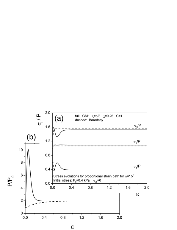
Figure 4: (a) Evolution of the stress eigenvalues (normalized by the pressure $P$) with the total strain $\varepsilon$, as obtained with gsh (full) and Barodesy (dashed). (b) Evolution of $P$ (normalized by the initial pressure $P_{0}$) with $\varepsilon$. The Barodesy curve is monotonic, The gsh one is not. This explains the difference in the transient regime.

Although the expressions from barodesy, Eqs.(53,54), and gsh, Eq.(47,48), are rather different, the relevant plots are not. Yet to achieve this agreement, hardly any fiddling with the parameters was necessary. The Barodesy parameters were simply taken from Eq.(23); the gsh parameters are essentially the same as we employed them before: $\xi,\chi$ are part of the energy and represent static parameters. We took $\xi=5/3$ as we have mostly done before, and took $\chi=0.26$. (In 3inv , we took $\chi=0.2$. This slight change perfected the agreement of Fig.1 that we could not resist.) We also took $C\equiv\Lambda\lambda_{1}/\left(\lambda\alpha_{1}\right)=1$ here. Previously, we equivalently took $\Lambda\equiv\lambda\sqrt{\eta_{1}/\gamma_{1}}\sim 114$, $\lambda_{1}\sim 3\lambda/10$, and $\alpha_{1}\sim 33$ in JL3 ; critState , separately.

V Strain Paths with density Change

Figure 5: The relation between the void ratio $e$ and the stress magnitude $\sigma$ of the asymptotic state (normalized by $\sigma$ at $e=0.65$), as given respectively by gsh and barodesy. With $v_{\ell\ell}\not=0$, the two quantities $e$ and $\sigma$ will change in tandem, according to either of these two curves.

If the strain path contains a small $v_{\ell\ell}$, the density and void ratio will change, as will the magnitude of the stress, according to Eq.(19) in gsh, and to Eq.(22) in barodesy. Again, in spite of the different expressions, the curves are similar, at least qualitatively, see Fig.(5). The convergence onto the asymptotic state is depicted in Fig.(6). Following Kolymbas’ papers, we have also computed 4 figures each for (drained) triaxial and oedometric tests employing gsh, see Fig.7 and 8.

Figure 6: Circumstances are the same as in Fig.3, except that, first, $v_{kk}\not=0$ and the density varies linearly, as given in the inset of (b). Second, only the gsh curve is displayed, not the Barodesy one (because given Fig.4,5, they cannot be that different). Convergence of the stress ratios takes place quickly, from where on the stress path is proportional. The first part of the pressure change occurs during the convergence, the second part, where the pressure change associated with positive and negative $v_{kk}$ diverge, belongs to the asymptotic state.

Figure 7: In the geometry of triaxial tests, various quantities are computed employing gsh, as functions of the strain $\varepsilon_{xx}$, holding $\sigma_{xx}=\sigma_{yy}$ constant. (The axial direction is $z$. The case with an initially higher density is rendered in solid lines, the looser one in dashed lines.) These are: (a) deviatoric stress $q\equiv\sigma_{zz}-\sigma_{xx}$; (b) void ratio $e$; (c) volumetric strain $\varepsilon_{v}$; (d) the friction ange, $\sin\phi_{m}\equiv q/\left(2\sigma_{xx}+q\right)$. We chose: $\alpha,\alpha_{1},\lambda\sim\left(1-\rho/\rho_{cp}\right)^{1.6}$ and $\eta_{1},\gamma_{1}\sim\left(1-\rho/\rho_{cp}\right)^{-1}$.

Figure 8: Oedometric test starting with an initially loose density, again computed with gsh. The following four quantities are calculated as functions of the axial $\sigma_{zz}$ while holding the lateral strain $\varepsilon_{xx}=\varepsilon_{yy}$ fixed: (a) $\varepsilon_{zz}$ of a axial stress-strain curve; (b) $\sigma_{xx}$ of a stress path; (c) $\varepsilon_{zz}$ versus time; (d) void ratio $e$ versus time. Note $\varepsilon_{zz}$ moving upwards implies a compaction of the system.

VI Conclusion

In comparing gsh to barodesy, we set out to achieve two goals: To validate gsh, and to provide a transparent, sound understanding for gr. Both goals were reached. gsh is validated because it yields similar results for various key quantities as barodesy, achieving better agreement than would be reasonably expected, without much fiddling with parameters.

Conversely, the understanding of Goldscheider Rules and Barodesy comes from the physics of gsh. The theory has (for the range of shear rates typical of soil mechanical experiments) three state variables and two constituent parts. The state variables are the density $\rho$, granular temperature $T_{g}$ (quantifying granular jiggling), and the elastic strain tensor $\hat{u}$ (accounting for the coarse-grained deformation of the grains). The two constituent parts are first the explicit expression of the stress tensor $\hat{\sigma}$, a function of $\hat{u},\rho$ that is obtained from the elastic energy; and second a rate-independent relaxation equation for $\hat{u}$, derived from the notion of variable transient elasticity. Given any initial $\hat{u}_{0}$, the system will always converge onto the stationary solution $\hat{u}^{c}$ as prescribed by the relaxation equation. $\hat{u}^{c}$ is a function of the constant strain rate, or equivalently, of the proportional strain path’s direction, and may be identified as the asymptotic, critical state for isochoric paths, $v_{\ell\ell}=0$. This convergence, a consequence of the relaxation equation, is closely related to variable transient elasticity, and hence a generic aspect of granular behavior.

Given $\hat{u}^{c}$ and the density, the stress is also fixed. Its form, however, depends on the expression for the elastic energy that is material dependent and less robust. If the strain path ${\hat{v}^{*}}\,t$ is isochoric, with $v_{\ell\ell}=0$, the asymptotic stress state is a constant of time, but a function of $\hat{u}^{c}$, or equivalently, of the strain path’s direction. As the path varies, the associated stress states lie within a triangle, as depicted in Fig.2.

If the shear rate is a sum of ${\hat{v}^{*}}\,t$ and a small $v_{\ell\ell}$, the asymptotic state is (cum grano salis) still given by the $\hat{u}^{c}$ associated with ${\hat{v}^{*}}\,t$, though the density will now change. The asymptotic stress is therefore a function of the same $\hat{u}^{c}$ and a changing density, hence no longer a constant. That the stress path is also proportional, that only the magnitude of the stress changes with time, not the ratios of its eigenvalues, is the least robust part of gr, because it depends on the density dependence of certain coefficients canceling.

Constructing a constitutive relation, specifying $(\partial_{t}+v_{k}\nabla_{k})\hat{\sigma}={\mathfrak{C}}(\hat{\sigma},\hat{v},\rho)$, is only for someone with vast experience with granular media and deep knowledge of how they behave. That gsh – derived from two simple notions of what the two basic elements of granular physics are – yields an equivalent account, is eye-opening, and the actually amazing fact of the presented agreement.

Appendix A Tensor decomposition

A $3\times 3$ symmetric tensor, e.g. the stress tensor $\sigma_{ij}$, can be decomposed into two parts: a spatial rotation $\widehat{O}$ and a part which is invariant under any rotation. In most analysis we are interested mainly in the three invariants. There are usually various ways to represent the invariant triplet. One of which is

$$P \equiv \sigma_{kk}/3,$$ (55)

$$\sigma_{s} \equiv \sqrt{\sigma_{lk}^{\ast}\sigma_{lk}^{\ast}},$$ (56)

$$\sigma_{t} \equiv \sqrt[3]{\sigma_{ik}^{\ast}\sigma_{kj}^{\ast}\sigma_{ji}^{\ast}}.$$ (57)

Another is $\left(P,L,\zeta\right)$ where

$$L \equiv \frac{1}{3}\arcsin\left(\sqrt{6}\frac{\sigma_{t}^{3}}{\sigma_{s}^{3}}\right),$$ (58)

$$\zeta = \arctan\left(\frac{\sigma_{s}}{\sqrt{3}P}\right)=\arcsin\left(\frac{\sigma_{s}}{\sigma}\right)=\arccos\left(\sqrt{3}\frac{P}{\sigma}\right),$$ (59)

are two angle variables ($\sigma\equiv\sqrt{\sigma_{lk}\sigma_{lk}}=\sqrt{\sigma_{s}^{2}+3P^{2}}$). In soil mechanics $L$ is usually called the Lode angle of stress. The angle $\zeta$ can be interpreted as a ”friction angle” (because it represents the ratio between shear force and pressure). Moreover we can also use the three eigenvalues $\left(\sigma_{1},\sigma_{2},\sigma_{3}\right)$ of the stress tensor as an invariant triplet, which are related to $\left(P,\sigma_{s},\sigma_{t}\right)$ by

$$\sigma_{1} = P+\frac{2\sigma_{s}}{\sqrt{6}}\sin\left(L-\frac{\pi}{3}\right),$$ (60)

$$\sigma_{2} = P-\frac{2\sigma_{s}}{\sqrt{6}}\sin L,$$ (61)

$$\sigma_{3} = P+\frac{2\sigma_{s}}{\sqrt{6}}\sin\left(L+\frac{\pi}{3}\right),$$ (62)

where $L$ is given by (58). In soil mechanics, it is also usual to define the two coordinates $\left(\pi_{1},\pi_{2}\right)$ in the so called $\pi$-plane,

$$\pi_{1} = \frac{\sigma_{3}-\sigma_{2}}{\sqrt{2}P},$$ (63)

$$\pi_{2} = \frac{2\sigma_{1}-\sigma_{2}-\sigma_{3}}{\sqrt{6}P}.$$ (64)

Inserting (60,61,61) into (63,64), we have

$$\pi_{1} = \frac{\sigma_{s}}{P}\sin\left(L+\frac{\pi}{6}\right),$$ (65)

$$\pi_{2} = -\frac{\sigma_{s}}{P}\cos\left(L+\frac{\pi}{6}\right).$$ (66)

With the help of Eqs.(55-66) we can readily transform among the invariant triplets: $\left(P,\sigma_{s},\sigma_{t}\right)$, $\left(P,L,\zeta\right)$, $\left(\sigma_{1},\sigma_{2},\sigma_{3}\right)$, $\left(P,\pi_{1},\pi_{2}\right)$. Similar decompositions apply for the elastic strain $u_{ij}$, total strain , strain rate tensor $v_{ij}$ etc., only note that the first invariant is frequently defined with a factor different from that of $P$.

References

- (1) G. Gudehus. Physical Soil Mechanics. Springer SPIN, 2010.
- (2) D. M. Wood. Soil Behaviour and Critical State Soil Mechanics. Cambridge University Press, 1990.
- (3) Goldscheider M. Grenzbedingung und Fließregel von Sand. Mechanics Research Communication (1976); 3:463–468.
- (4) Kolymbas D. Barodesy: a new constitutive frame for soils. Geotechnique Letters 2, 17–23, (2012), http://dx.doi.org/10.1680/geolett.12.00004; Barodesy: A new hypoplastic approach. International Journal for Numerical and Analytical Methods in Geomechanics (2011). doi:10.1002/nag.1051; Sand as an archetypical natural solid. In Mechanics of Natural Solids, Kolymbas D, Viggiani G (eds.). Springer: Berlin, (2009); 1–26;
- (5) D. Kolymbas. Introduction to Hypoplasticity. Balkema, Rotterdam, 2000. W. Wu and D. Kolymbas. Constitutive Modelling of Granular Materials. Springer, Berlin, 2000.
- (6) Y.M. Jiang and M. Liu, Granular solid hydrodynamics. Granular Matter, 11, 139 (2009); Y.M. Jiang and M. Liu, The Physics of Granular Mechanics. Mechanics of Natural Solids, edited by D. Kolymbas and G. Viggiani, Springer, pp. 27–46 (2009); G. Gudehus, Y.M. Jiang, and M. Liu, Seismo- and thermodynnamics of granular solids. Granular Matter, 1304, 319 (2011).
- (7) D.O. Krimer, M. Pfitzner, K. Bräuer, Y. Jiang, M. Liu. Granular elasticity: General considerations and the stress dip in sand piles. Phys. Rev. E74, 061310 (2006).
- (8) K. Bräuer, M. Pfitzner, D.O. Krimer, M. Mayer, Y. Jiang, M. Liu. Granular elasticity: Stress distributions in silos and under point loads. Phys. Rev. E74, 061311 (2006);
- (9) Y.M. Jiang, M. Liu. Eur. A brief review of granular elasticity. Phys. J. E 22, 255 (2007).
- (10) Y.M. Jiang, M. Liu. Incremental stress-strain relation from granular elasticity: Comparison to experiments. Phys. Rev. E 77, 021306 (2008).
- (11) Y.M. Jiang, M. Liu. Energetic Instability Unjams Sand and Suspension. Phys. Rev. Lett. 93, 148001(2004).
- (12) Y.M. Jiang, H.P. Zheng, Z. Peng, L.P. Fu, S.X. Song, Q.C. Sun, M. Mayer, and M. Liu, Expression for the granular elastic energy. Phys. Rev. E 85, 051304 (2012)
- (13) M. Mayer and M. Liu. Propagation of elastic waves in granular solid hydrodynamics. Phys. Rev. E, 82:042301, 2010.
- (14) Y.M. Jiang, M. Liu. From elasticity to hypoplasticity: Dynamics of granular solids. Phys. Rev. Lett. 99, 105501 (2007).
- (15) Stefan Mahle, Yimin Jiang, and Mario Liu. The Critical State and the Steady-State solution in Granular Solid Hydrodynamics. arXiv:1006.5131v3 [physics.geo-ph], 2010.
- (16) Stefan Mahle, Yimin Jiang and Mario Liu. Granular Solid Hydrodynamics: Dense Flow, Fluidization and Jamming. arXiv:1010.5350v1 [cond-mat.soft], 2010.
- (17) Samimi, A.; Hassanpour, A., and Ghadiri, M. Single andbulk compressions of soft granules: Experimental studyand DEM evaluation. Chemical Engineering Science, 60(14):3993-4004, 2005.
- (18) Philippe, P.; Bonnet, F., and Nicot, F. Settlement of a granular material: boundary versus volume loading. Granular Matter, 13(5):585-598, 2011.
- (19) Ezaoui, A. and Di Benedetto, H. Experimental measurements of the global anisotropic elastic behaviour of dry Hostun sand during triaxial tests, andeffect of sample preparation. Géotechnique, 59(7):621-635, 2009.
- (20) Sun, J. and Sundaresan, S. A constitutive model with microstructure evolution for ow of rate independent granular materials. Journal of Fluid Mechanics, 682:590-616, 2011.
- (21) Schwedes, J. Review on testers for measuring flow properties of bulk solids. Granular Matter, 5(1):1-43, 2003.
- (22) Luding, S. and Alonso-Marroquín, F. The critical-state yield stress (termination locus) of adhesive powders from a single numerical experiment. Granular Matter, 13(2):109-119, 2011.
- (23) Makse, H. A.; Johnson, D. L., and Schwartz, L. M. Packing of compressible granular materials. Phys. Rev. Lett., 84(18):4160-4163, 2000.
- (24) Masín, D. Asymptotic behaviour of granular materials. Granular Matter, (in press), 2012.
- (25) Saadatfar, M.; Sheppard, A. P.; Senden, T. J., andKabla, A. J. Mapping forces in a 3D elastic assembly of grains. Journal of the Mechanics and Physics of Solids, 60(1):55-66, 2012.
- (26) Barreto, D. and O’Sullivan, C. The influence of inter-particle friction and the intermediate stress ratio on soil response under generalised stress conditions. Granular Matter, 14(4):505-521, 2012.
- (27) Thornton, C. Quasi-static simulations of compact polydisperse particle systems. Particuology, 8(2):119-126, 2010.
- (28) Thornton, C. and Anthony, S. J. Quasistatic deformation of particulate media. Philosophical Transactions of the Royal Society of London. Series A: Mathematical, Physical and Engineering Sciences, 356(1747): 2763-2782, 1998.
- (29) Thornton, C. and Zhang, L. A numerical examination of shear banding and simple shear non-coaxial flow rules. Philosophical Magazine, 86(21-22):3425-3452, 2006.
- (30) Thornton, C. and Zhang, L. On the evolution of stressand microstructure during general 3D deviatoric straining of granular media. Géotechnique, 60(5):333-341, 2010.
- (31) Yimsiri, S. and Soga, K. DEM analysis of soil fabric effects on behaviour of sand. Géotechnique,, 60(6), 2010.
- (32) Zhao, X. and Evans, T. M. Numerical analysis of critical state behaviors of granular soils under different loading conditions. Granular Matter, 13(6):751-674, 2011.
- (33) G. T. Houlsby and A. M. Puzrin. Principles of Hyperplasticity. Springer (2006).
- (34) S. R. de Groot and P. Masur, Non-Equilibrium Thermodynamics, (Dover, New York 1984).
- (35) B.O. Hardin and F.E. Richart. Elastic wave velocities in granular soils. J. Soil Mech. Found. Div. ASCE, 89: SM1:33–65, 1963.