From creeping to inertial flow in porous media: a lattice Boltzmann - Finite Element study

Abstract

The lattice Boltzmann method has been successfully applied for the simulation of flow through porous media in the creeping regime. Its technical properties, namely discretization, straightforward implementation and parallelization, are responsible for its popularity. However, flow through porous media is not restricted to near zero Reynolds numbers since inertial effects play a role in numerous natural and industrial processes. In this paper we investigate the capability of the lattice Boltzmann method to correctly describe flow in porous media at moderate Reynolds numbers. The selection of the lattice resolution, the collision kernel and the boundary conditions becomes increasingly important and the challenge is to keep artifacts due to compressibility effects at a minimum. The lattice Boltzmann results show an accurate quantitative agreement with Finite Element Method results and evidence the capability of the method to reproduce Darcy’s law at low Reynolds numbers and Forchheimer’s law at high Reynolds numbers.

I Introduction

Predicting the transport properties of porous media, like the fluid permeability, defined by Darcy’s law, or heat conductivity, is of paramount importance in chemical, mechanical, geological, environmental and petroleum industries. Flow situations in porous media are not restricted to the creeping flow regime, i.e., near zero Reynolds numbers where Darcy’s law applies Bear:1972 . Many important natural and industrial processes are characterized by large Reynolds numbers, where inertial effects also play a role. Examples include gas flow through a catalytic converter, groundwater flow, filtration processes and the flow of air in our lungs MPT_2009 . Hence, accurate simulation methods are needed to improve our understanding of these processes.

The lattice Boltzmann (LB) method has become an efficient tool bib:ferreol-rothman ; 1990PhFl.2.2085C ; bib:qian-dhumieres-lallemand as an alternative to a direct numerical solution of the Navier-Stokes equation PhysRevB.46.6080 ; MAKHT02 for simulating fluid flow in complex geometries such as porous media. Historically, the LB method was developed from the lattice gas automata bib:qian-dhumieres-lallemand ; bib:succi-01 , replacing the number of particles in each lattice direction with the ensemble average of the single particle distribution function, and the discrete collision rule with a linear collision operator. In the LB method all computations involve local variables so that it can be parallelized easily MAKHT02 . Together with uniform grids and thus straightforward discretization, the LB method has become very popular in the field of porous media flow simulations. With the advent of more powerful computers it became possible to perform detailed simulations of finely resolved complex samples bib:aharonov-rothman ; bib:auzeraisGRL96 ; bib:ferreol-rothman ; 1990PhFl.2.2085C ; KL97 ; HKL01 ; bib:cf.CPaLLuCMi.2006 ; NZRHH10 ; NH10 ; MAKHT02 .

In this work we investigate the accuracy of the LB method in flow regimes beyond Darcy’s regime. We focus on limitations of the method with respect to the lattice resolution and the selection of parameters. In particular, we address the requirement of reducing undesired compressibility effects by keeping the Mach number low, and how this influences the achievable maximum Reynolds numbers. In order to keep the compressibility as moderate as possible a new simulation setup combining an injection channel, density boundary conditions, and an external body force for driving the fluid is introduced. Nevertheless, for high Reynolds numbers, a low fluid viscosity and high resolution are required. Thus, a thorough investigation of the impact of the compressibility on the measured permeability is presented.

To confirm the validity of the LB results, they are compared to Finite Element Method (FEM) simulations that are performed with the commercial software package ANSYS. During the past decades, the FEM has been widely used to simulate fluid flow through porous media. It is known that FEM can deal with complex pore geometries and boundary conditions, see for examples Refs. Zabaras ; girault ; thomasset . Tezduyar et al. Tezduyar have developed the so-called deforming-spatial-domain/space-time (DSD/ST) procedure for flow problems with deforming interfaces using the so-called Arbitrary Lagrangian-Eulerian (ALE) methods and a space-time finite element method. This approach was based on fully resolved simulations around particles and therefore computationally expensive in dense flows. For an overview of some finite element and finite difference techniques for incompressible fluid flow see Ref. Fletcher and for the efficiency of the solution algorithms Ref. Turek . In recent studies, Yazdchi et al. relate the macroscopic properties of porous media, namely permeability and inertial coefficients, to their microstructure and porosity kazemluding ; kazemluding2 .

The remainder of this article is organised as follows: In section II, an introduction to porous media flow including laminar and weakly inertial flow, i.e. creeping flow, named Darcy’s flow, and Forchheimer’s flow is given, respectively. In section III, the LB and FEM methods are introduced along with the description of the simulation setup. In section IV, we demonstrate quantitative agreement of LB and FEM simulations with theoretical predictions for fluid flow in porous media in the above mentioned regimes. Finally we analyze and compare the results before we conclude.

II Porous media flow

Weak inertial flow, also named creeping flow (near zero Reynolds numbers) in porous media, can be described by Darcy’s law bib:darcy ; Dullien:1992 . It is defined by

$$\kappa=-\mu\frac{{u_{\rm s}}}{\langle(\nabla p)_{x_{2}}\rangle},$$ (1)

where the porous medium parameter $\kappa$ (always positive) is named the permeability of the medium. $\langle(\nabla p)_{x_{2}}\rangle$ represents the average pressure gradient in the direction of the flow $x_{2}$, see Fig. 1, and $\mu$ represents the dynamic viscosity of the fluid. ${u_{\rm s}}$ represents the superficial velocity defined by

$${u_{\rm s}}=\frac{1}{V_{\rm t}}\int_{V_{\rm f}}u_{2}\,{\rm d}{V},$$ (2)

where $u_{2}$ is the fluid velocity in the flow direction. $V_{\rm t}$ and $V_{\rm f}$ represent the total volume and the fluid volume, respectively. The average velocity within the porous medium $\langle u\rangle$ is related to the superficial velocity by ${u_{\rm s}}=\varepsilon\langle u\rangle$, where $\varepsilon$ is the porosity of the medium. According to Eq. (1), Darcy’s law corresponds to a linear relation between the average pressure gradient $\langle(\nabla p)_{x_{2}}\rangle$ and the superficial velocity ${u_{\rm s}}$, in the literature also referred to as seepage velocity MA91 . Darcy’s law was obtained empirically in 1846, but it can be derived from the continuous moment and mass balance assuming that the solid-fluid hydrodynamic interaction is proportional to the relative solid-fluid velocity Mass1984 .

When the Reynolds number is increased, inertia effects become relevant ($\text{Re}\approx\mathcal{O}(1)$). The average pressure gradient $\langle(\nabla p)_{x_{2}}\rangle$ and the superficial velocity ${u_{\rm s}}$ do not follow a linear relation anymore as it was empirically shown by Forchheimer Forchh01 ; ACAMS_1999 . For this flow regime, named Forchheimer’s regime, a quadratic term in ${u_{\rm s}}$ is included to take into account the inertia effects. According to Massarani Mass1984 , Forchheimer’s law can be written as

$$\langle(\nabla p)_{x_{2}}\rangle=-\left(\frac{\mu}{\kappa}+\frac{\hat{\rho}\!_{\circ}c}{\sqrt{\kappa}}{u_{\rm s}}\right){u_{\rm s}},$$ (3)

where $c$ is a positive dimensionless parameter and $\hat{\rho}\!_{\circ}$ is the reference fluid density. The quadratic term in Eq. (3) describes a linear relationship between the solid-fluid hydrodynamic interaction and the relative solid-fluid velocity. Darcy’s law is recovered in the limit of ${u_{\rm s}}\rightarrow$0.

A transition from creeping flow to inertial flow has been reported in many studies, see for example the work of Koch and Ladd on flow in a random array of cylinders KL97 and spheres HKL01 . Also the existence of a transition regime between the creeping and inertial regimes has been reported in the past SA99 . This departure from Darcy’s regime is of the order of ${u_{\rm s}}^{3}$ kazemluding ; AGO07 ; WL91 ; MA91 ; FGQ97 and the relation between $\langle(\nabla p)_{x_{2}}\rangle$ and ${u_{\rm s}}$ in this short interval is then given by

$$\langle(\nabla p)_{x_{2}}\rangle=-\left(\frac{\mu}{\kappa}+\frac{\gamma{\hat{\rho}\!_{\circ}}^{2}}{\mu}{u_{\rm s}}^{2}\right){u_{\rm s}},$$ (4)

where the cubic term in ${u_{\rm s}}$ with positive parameter $\gamma$ represents the weak inertia correction.

III Simulation methods

III.1 The lattice Boltzmann Method

The integration of the Boltzmann equation on a regular lattice using a discrete set of velocities ${\bf c}_{{\dot{\imath}}}$ defines the lattice Boltmann method. The lattice is defined by the spacing $\Delta x$, with the discrete velocity in units of $\Delta x/\Delta t$, where $\Delta t$ represents the timestep. Thus, the basic differential equation for the method is

$$f_{{\dot{\imath}}}(\mathbf{x}+\Delta t\,{\bf c}_{{\dot{\imath}}},t+\Delta t)-f_{{\dot{\imath}}}(\mathbf{x},t)=-\frac{\Delta t}{\tau}\left(f_{{\dot{\imath}}}(\mathbf{x},t)-f^{\rm eq}_{{\dot{\imath}}}(\mathbf{x},t)\right),$$ (5)

where $f_{{\dot{\imath}}}(\mathbf{x},t)$ represents the number of particles moving at position $\mathbf{x}$ with velocity ${\bf c}_{{\dot{\imath}}}$ at discrete time $t$. The term on the right hand side represents the collision operator as introduced by Bhatnagar, Gross and Krook (BGK) bib:chen-chen-martinez-matthaeus ; bib:bgk , which approximates the collision through a linearization towards the equilibrium distribution function $f^{\rm eq}_{{\dot{\imath}}}(\mathbf{x},t)$ with a unique relaxation time $\tau$. This value is restricted to $\tau/\Delta t>1/2$ assuring positive viscosity. If $\tau/\Delta t$ approaches $1/2$ numerical instabilities can arise Sterling:1996:SAL:227647.227666 . This collision operator is often referred to as “single relaxation time” or BGK model. Under the assumption of very low Knudsen and Mach numbers ($\rm Ma$) which assures small compressibility effects, $f^{\rm eq}_{{\dot{\imath}}}(\mathbf{x},t)$ is calculated by a second order Taylor expansion of the Maxwell distribution as bib:qian-dhumieres-lallemand

$$f^{\rm eq}_{{\dot{\imath}}}(\mathbf{x},t)=\omega_{{\dot{\imath}}}\frac{\rho}{{\rho\!_{{}_{\circ}}}}\left(1+\frac{\mathbf{u}\cdot{\bf c}_{{\dot{\imath}}}}{{{c_{\rm s}}}^{2}}+\frac{(\mathbf{u}\cdot{\bf c}_{{\dot{\imath}}})^{2}}{2{{c_{\rm s}}}^{4}}-\frac{\mathbf{u}\cdot\mathbf{u}}{2{{c_{\rm s}}}^{2}}\right).$$ (6)

${\rho\!_{{}_{\circ}}}$ is a reference density. The coefficients $\omega_{{\dot{\imath}}}$ are called lattice weights and are chosen to assure conservation of mass and momentum. They differ with lattice type, number of space dimensions and number of discrete velocities. For the cubic fashion 3D lattice with 19 discrete velocities ($i=0,..,18$) used in this work they are $1/3$, $1/18$ and $1/36$ for the rest particles, the particles moving parallel to the $x_{1}$, $x_{2}$, or $x_{3}$, and the particles moving in diagonal directions, respectively bib:qian ; bib:qian-dhumieres-lallemand . Even though the system of interest in this paper is intrinsically two-dimensional, we apply a three-dimensional implementation of the LB method and compute the flow in a very flat simulation domain with periodic boundary conditions in the $x_{3}$ direction. We do not expect this to have any influence on the simulation results, but it allows us to use our well tested implementation “LB3D”. The only disadvantage are higher computational costs, but we do not report on the amount of CPU time required for a given flow problem in this paper.

No-slip boundary conditions on the solid walls are implemented by mid-plane bounce back rules SukopThorne2007 . The BGK model is known to suffer from an artificial viscosity dependent slip at boundaries if these boundary conditions are used. An alternative approach for the collision operator, which reduces this well known drawback of the BGK model, is the multi relaxation time (MRT) method bib:cf.CPaLLuCMi.2006 ; NZRHH10 . Here, the right hand side of Eq. (5) is replaced by the expression

$$-\Delta t\left[{\mathbf{M}}^{-1}\cdot\mathbf{\check{S}}\cdot\left(\mathbf{m}(\mathbf{x},t)-{\mathbf{m}}^{\mathrm{eq}}(\mathbf{x},t)\right)\right]_{{\dot{\imath}}},$$ (7)

where $\mathbf{M}$ is a linear transformation chosen such that the moments

$$m_{{\dot{\imath}}}(\mathbf{x},t)=\sum_{{\dot{\jmath}}}M_{{\dot{\imath}}\,{\dot{\jmath}}}\,f_{{\dot{\jmath}}}(\mathbf{x},t)$$ (8)

represent hydrodynamic modes of the problem. We use the definitions given in 2002RSPTA.360..437D , where $m_{0}$ is the fluid density, $m_{2}$ represents the kinetic energy, $m_{{\dot{\imath}}}$ with ${\dot{\imath}}=3,5,7$ is the momentum flux and $m_{{\dot{\imath}}}$, with ${\dot{\imath}}=9,11,13,14,15$ are components of the symmetric traceless viscous stress tensor. During the collision step the density and the momentum flux are conserved so that $m_{{\dot{\imath}}}=m^{\mathrm{eq}}_{{\dot{\imath}}}$ with $i=0,3,5,7$. The non-conserved equilibrium moments $m^{\mathrm{eq}}_{{\dot{\imath}}}$, $i\neq 0,3,5,7$, are assumed to be functions of these conserved moments and explicitly given in 2002RSPTA.360..437D . $\mathbf{\check{S}}$ is a diagonal matrix $\check{S}_{{\dot{\imath}}\,{\dot{\jmath}}}=\check{s}_{{\dot{\imath}}}\,\delta_{{\dot{\imath}}\,{\dot{\jmath}}}$. The diagonal elements $\tau_{{\dot{\imath}}}=1/\check{s}_{{\dot{\imath}}}$ in the collision matrix are the relaxation time of the moment $m_{{\dot{\imath}}}$. One has $\check{s}_{0}=\check{s}_{3}=\check{s}_{5}=\check{s}_{7}=0$, because the corresponding moments are conserved. $\check{s}_{1}=1/\tau_{\rm bulk}$ describes the relaxation of the energy and $\check{s}_{9}=\check{s}_{11}=\check{s}_{13}=\check{s}_{14}=\check{s}_{15}=1/\tau$ the relaxation of the stress tensor components. The remaining diagonal elements of $\mathbf{\check{S}}$ are chosen such that one has

$$\begin{split}\mathbf{\check{S}}={\rm diag}&(0,1/\tau_{\rm bulk},1.4,0,1.2,0,1.2,0,1.2,1/\tau,\\ &1.4,1/\tau,1.4,1/\tau,1/\tau,1/\tau,1.98,1.98,1.98),\end{split}$$ (9)

to optimize the algorithm performance 2000PhRvE..61.6546L ; 2002RSPTA.360..437D . The two relaxation times $\tau$ and $\tau_{\rm bulk}$, are restricted as well as for the BGK method to be $>\Delta t/2$, but allow to define the kinematic and bulk viscosity, respectively. This multi relaxation time scheme is commonly referred to as “two relaxation time” (TRT) method. An alternative TRT implementation can be found in el00178 ; el00173 .

The macroscopic density $\rho(\mathbf{x},t)$ and velocity $\mathbf{u}(\mathbf{x},t)$ are obtained from $f_{{\dot{\imath}}}(\mathbf{x},t)$ as

$$\rho(\mathbf{x},t) = {\rho\!_{{}_{\circ}}}\sum_{{\dot{\imath}}}f_{{\dot{\imath}}}(\mathbf{x},t),$$ (10)

$$\mathbf{u}(\mathbf{x},t) = \frac{{\rho\!_{{}_{\circ}}}}{\rho(\mathbf{x},t)}\sum_{{\dot{\imath}}}f_{{\dot{\imath}}}(\mathbf{x},t)\,{\bf c}_{{\dot{\imath}}}.$$ (11)

The pressure is given by

$$p(\mathbf{x},t)={{c_{\rm s}}}^{2}\,\rho(\mathbf{x},t),$$ (12)

where ${c_{\rm s}}=1/\sqrt{3}(\Delta x/\Delta t)$ is the speed of sound bib:qian-dhumieres-lallemand ; bib:succi-01 . The kinematic viscosity of the fluid $\nu=\mu/\rho$ is a function of the discretization parameters, $\Delta x$ and $\Delta t$, and the relaxation time $\tau$ bib:chapman-cowling ; Wolf05 . It is given by

$$\nu=\frac{{c_{\rm s}}^{2}\,\Delta t}{2}\left(2\frac{\tau}{\Delta t}-1\right).$$ (13)

III.2 The Finite Element Method

The velocity and pressure profiles through the system can be obtained from the solution of the conservation laws, namely, the continuity equation (conservation of mass) and the Navier-Stokes equations (conservation of momentum). In the absence of body forces, but assuming a constant density (i.e. incompressible flow) and steady state flow conditions, the equations of conservation of mass and momentum for a Newtonian fluid are simplified to

$$\nabla\cdot\mathbf{u} = 0,$$ (14)

$$\rho(\mathbf{u}\cdot\nabla\mathbf{u}) = -\nabla p+\mu\nabla^{2}\mathbf{u}.$$ (15)

The FEM makes use of the variational formulations that allow the transformation of the above equations into a system of linear algebraic equations, which can be solved using a simple LU decomposition or iterative algorithms Kandhai_1999 ; saurabh_2012 . Stable discretizations of the above equations are difficult to construct and it is known that the incompressibility constraint is not strongly enforced when using continuous polynomial shape functions for pressure. See Turek for a detailed theory and discussion. Langtangen et al. present an overview of the most common numerical solution strategies, including fully implicit formulations, artificial compressibility methods, penalty formulations and operator splitting methods Langtangen . Using the conventional FEM scheme, we solve the above equations with the commercial software ANSYS bib:Yazdchia . The nonlinear solution procedure used in ANSYS belongs to a general class of Semi-Implicit Methods for Pressure Linked Equations (SIMPLE). On the flow domain, the steady state Navier-Stokes equations combined with the continuity equations are discretized into linear triangular elements. They are then solved using a segregated sequential solution algorithm. This means that element matrices are formed, assembled and the resulting system is solved using the Gaussian elimination algorithm for each degree of freedom separately. The number of iterations required to achieve a converged solution may vary considerably, depending on the number of elements, inertial contribution and the stability of the problem. Some more technical details are given in bib:Yazdchia .

By knowing the fluid velocity field, the superficial velocity is then calculated from Eq. (2). Recently, using FEM simulations, Yazdchi and Luding kazemluding show that for both ordered and random fibre arrays, the weak inertia correction to the linear Darcy relation is third power in superficial velocity, up to small Re $\approx$ 1-5. When attempting to fit the data with a particularly simple relation, a non-integer power law performs astonishingly well up to the moderate Re $\approx$ 30.

A typical unstructured, fine and triangular FEM mesh is shown in Fig. 1. The mesh size effect is examined by comparing the simulation results for different resolutions. The mesh refinement is done on element level, meaning that a finer grid is overlaid on the coarse one. In order to be able to apply periodic boundary conditions in $x_{1}$ direction, see Fig. 1, we discretize the system such that we come up with the same number of nodes on the left and right boundary. Periodic boundary conditions are applied by setting additional constrains, i.e. same velocity, on these nodes.

III.3 Computational Domain and Simulation Setup

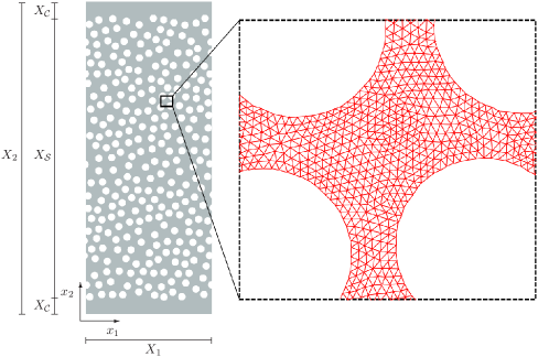
Figure 1: Computational domain with dimensions $X_{1}\times X_{2}$ ($X_{1}=0.4\,X_{2}$). The sample is composed of 266 circles with radius $r$ representing 1.25% of $X_{2}$. They are randomly distributed assuring a minimum circle center distance $\Delta_{\min}$ of 3.125% of $X_{2}$. Pure fluids chambers with length of 5% of $X_{2}$ are placed after and before the sample. The right inset shows a zoom of a typical unstructured, fine and triangular FEM mesh.

The computational domain is presented in Fig. 1. The porous sample has a length of $X_{\mathcal{S}}$ representing $0.9\,X_{2}$, and it is composed of 266 circles, randomly distributed with a radius $r$ of 1.25% of $X_{2}$. A minimum distance $\Delta_{\min}$ of 3.125% of $X_{2}$ is imposed between the circle centers. The sample porosity then follows to be $\varepsilon=0.63730$.

For the LB method three different resolutions are used, namely low resolution (L), intermediate resolution (M), and high resolution (H), see Table. 1 for details. For the FEM method also three resolutions are used, corresponding to 22048, 49670, and 982376 triangular elements, respectively. These meshes are referred to using the same abbreviations as for the LB simulations. However, one should keep in mind that the number of discretisation elements used in both methods cannot be compared easily since the LB simulations utilize a regular Cartesian lattice, while the FEM simulations are based on unstructured grids with locally varying resolution.

Table 1: Domain discretization for the LB simulations.

Resolution	$\displaystyle{\frac{\displaystyle{X_{1}}}{\displaystyle{\Delta x}}}$	$\displaystyle{\frac{\displaystyle{X_{2}}}{\displaystyle{\Delta x}}}$	$\displaystyle{\frac{\displaystyle{X_{\mathcal{S}}}}{\displaystyle{\Delta x}}}$	$\displaystyle{\frac{\displaystyle{X_{\mathcal{C}}}}{\displaystyle{\Delta x}}}$	$\displaystyle{\frac{\displaystyle{r}}{\displaystyle{\Delta x}}}$	$\displaystyle{\frac{\displaystyle{\Delta_{\min}}}{\displaystyle{\Delta x}}}$
low (L)	128	320	288	16	4	10
medium (M)	256	640	576	32	8	20
high (H)	512	1280	1152	64	16	40

In the LB simulations a constant acceleration $\mathbf{g}=g\mathbf{e}_{2}$ drives the fluid using Guo’s method Guo02 . This acceleration defines the pressure gradient and acts on the fluid inside the sample, i.e. from $x_{2}=X_{\mathcal{C}}$ to $x_{2}=X_{\mathcal{C}}+X_{\mathcal{S}}$. Together with this, on-site pressure boundary conditions are implemented on the inlet-plane $x_{2}=0$ and on the outlet-plane $x_{2}=X_{2}$ setting a constant density value ${\rho\!_{{}_{\circ}}}$ (reference density, i.e. $\sum f_{{\dot{\imath}}}=1$) on both planes. See Eq. (12) for the relation between the density and pressure within the LB method. These pressure boundary conditions are implemented using the method of Zou & He bib:pf.QZoXHe.1997 ; HH08b . Different values of the acceleration $g$ are used in order to study different Re regimes. In our earlier work we proposed to use just on-site pressure boundary conditions at the inlet- and outlet-planes, ($\sum f_{{\dot{\imath}}}=1+\delta$ and $\sum f_{{\dot{\imath}}}=1-\delta$, respectively) to impose a pressure drop of $2\delta$ NH10 . The here presented new setup allows to reduce compressibility effects inside the sample when the Reynolds number is increased. Periodic boundary conditions are applied in the $x_{1}$ direction.

In the FEM simulations, a pressure drop is imposed while the density is kept constant to drive the fluid. Further, we impose zero velocity on the surface of the fibres and also apply periodic boundary conditions in the $x_{1}$ direction.

IV Simulation Results

We present a detailed analysis of the simulation of porous media flow at low to moderate Reynolds numbers using the LB method. Special attention is given to its collision kernel, the discretization and the value of the relaxation time. To increase Re either the average flow velocity can be increased or the fluid viscosity can be decreased. However, the range of these parameters is limited: the lattice Boltzmann method is known to reproduce the Navier-Stokes equations in the low Mach number limit only, i.e., at high flow velocities compressibility artifacts can occur and render the results invalid. To validate the obtained data and to understand the impact of these limits on the precision of the LB results, we present a quantitative comparison with FEM results and theoretical predictions.

For the LB simulations $100,000$ timesteps assure the steady state. The superficial velocity defined by Eq. (2) is calculated from the steady state LB data by

$${u_{\rm s}}=\displaystyle{\frac{\displaystyle{(\Delta x)^{2}}}{\displaystyle{X_{1}\,X_{2}}}}\sum_{\mathbf{x}\in\mathcal{X}}u_{2}(\mathbf{x}),$$ (16)

where $\mathcal{X}$ represents all fluid nodes in the simulation domain. The average pressure gradient is expected to be

$$\langle(\nabla p)_{x_{2}}\rangle=-g{\rho\!_{{}_{\circ}}}.$$ (17)

The Mach and Reynolds numbers are defined by

$$\rm Ma = \frac{\langle u\rangle}{{c_{\rm s}}},$$ (18)

Re $$= \frac{\langle u\rangle\,r}{\nu}.$$ (19)

Fig. 2 shows the relative maximum fluid density as a measure for the compressibility. The data are obtained from LB-MRT simulations of flow in the model geometry introduced above. While the open symbols represent data obtained using standard pressure drop boundary conditions (see NH10 ), the closed symbols describe data obtained with the newly proposed simulation setup combining pressure boundary conditions with a body force $\mathbf{g}$. In Fig. 2 the compressibility and thus the increase of the relative maximum density in the system increases for higher Re. Further, a clear reduction of compressibility effects is obtained when the newly proposed simulation setup is used.

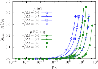
Figure 2: Normalized maximum fluid density as a measure for the effect of compressibility versus Reynolds number. Open symbols denote data obtained from LB-MRT simulations where the fluid is driven by an imposed pressure drop ($p$-BC) as suggested in NH10 . When combining a fixed density at the in- and outlet of the domain with a driving body force ($p$-BC + $\mathbf{g}$), compressibility effects can be reduced substantially. Together with low values of the relaxation time $\tau/\Delta t$ higher Re can be reached (solid symbols).

Fig. 2 also shows the effect of a reduced relaxation time (and thus viscosity) on the maximum reachable Re and the related compressibility effects. The compressibility of the fluid starts to become less important for lower viscosities and the combination of a low relaxation time ($\tau/\Delta t=0.6$) together with the combined pressure and body force boundary conditions leads to higher maximum Reynolds numbers. With this combination, Re of the order of 30 can be reached before, at large Re, fluctuations become too large for reliable analysis of the simulations.

Fig. 3 shows the permeability estimate obtained from LB simulations using different discretizations and collision kernels. In our previous work it was shown for BGK simulations of 3D Poiseuille flow that when a relaxation time close to $\tau/\Delta t=0.8$ is used, the dependency of the results on the discretization is minimal NZRHH10 . As it is also demonstrated in the same article, finding such an optimal value for the relaxation time is impossible for more realistic samples such as a discretized Fontainebleau sandstone or the array of cylinders as used here: a strong dependency on the discretization appears when the BGK model is used, even though the relaxation time is set to $\tau/\Delta t=0.8$. By using the MRT model this dependency can be decreased substantially. As can be observed in Fig. 3, the results of both collision kernels are qualitatively similar, i.e., both methods correctly reproduce the expected shape of the curve for comparable maximum Re. One can see that in the case of the low resolution sample (L) the departure from the Darcy’s regime (constant permeability) is to higher permeability values, which is unphysical since $c$ in Eq. (3) is a non-negative parameter. In the case of intermediate (M) and high resolution (H), the departure is to lower permeability values, but only using the high resolution sample it is possible to simulate high-enough Reynolds numbers to analyze this phenomenon.

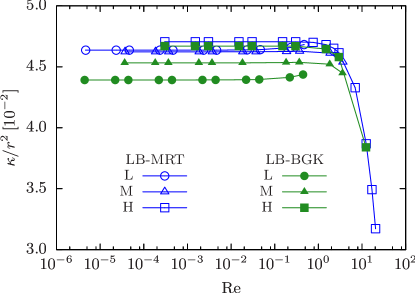
Figure 3: Resolution and collision kernel ($\tau/\Delta t=0.6$) analysis for permeability estimation vs. Re. The results show a dependency with the domain discretization, which is stronger when the BGK collision kernel is used.

Fig. 4 shows the permeability estimation for the LB-MRT method using different values for the relaxation time. Due the resolution used for this study (H) together with the MRT collision kernel it is not surprising that the results do not differ much quantitatively, but only by about 3%. The main difference is in the highest possible Reynolds numbers which can be reached by using a small value of the relaxation time $\tau/\Delta t=0.6$, in accordance with Fig. 2. As mentioned above numerical instability arises when the relaxation time approaches $\tau/\Delta t=0.5$. For this reason the smallest value used in this work is $\tau/\Delta t=0.6$.

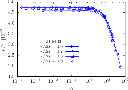
Figure 4: Relaxation time analysis for permeability estimation vs. Re calculated using the LB-MRT method and the high resolution (H) computational domain. Different values for the relaxation time $\tau/\Delta t$ were used. The results only differ by $\approx 3\%$ and the highest Re can be reached with the smallest value of $\tau/\Delta t=0.6$.

For porous media flow calculations using LB-MRT and $\tau/\Delta t=0.6$, Fig. 2 shows that at high Reynolds numbers the compressibility is of the order of 30%. Furthermore as we can see in Fig. 5 the superficial velocity remains low enough to keep Mach numbers below $\approx 10^{-1}$. However, inside the sample there are zones with high velocity. Indeed, for the two higher Reynolds numbers simulated, on $\approx 25\%$ and $\approx 45\%$ of the fluid nodes the velocity is higher than 20% of the speed of sound ${c_{\rm s}}$, see Fig. 5. Such high velocities and strong compressibility which are present at high Reynolds numbers highly question the validity of the results.

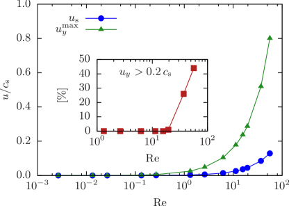
Figure 5: Superficial velocity ${u_{\rm s}}$ and maximal velocity $u_{y}^{\max}$ inside the sample for LB-MRT and $\tau/\Delta t=0.6$. The inset shows the percentage of fluid nodes with velocity $u_{y}$ higher than 20% of the speed of sound.

To investigate the validity of the results FEM simulations are performed as a benchmark for the LB simulations. In Fig. 6 the data obtained using both methods are plotted. One can see that the FEM results also show a dependence on the sample resolution. As stated above, in the case of the FEM the L, M, and H consist of domains with 22048, 49670, and 982376 elements. The resolution dependency is also demonstrated in the inset of the figure, where the permeability is shown as a function of resolution for a Reynolds number of $\text{Re}\approx 10^{-3}$. For simulations using $1\times 10^{6}$ elements, there is a difference of $\approx 2\%$ between LB and FEM results. This can be explained by several factors: neither FEM nor LB results are fully converged with respect to the required number of elements, but performing a large number of simulations with substantially higher resolution is not feasible with the computational resources available – in particular since the final values are expected to change by not more than a few percent. Since the LB results are systematically lower than the FEM results, a possible explanation can be the loss of accuracy of LB due to the relatively small choice for the relaxation time ($\tau/\Delta t=0.6$) as demonstrated in Fig. 4. In any case, the deviation is small and thus it can be concluded that the data in Fig. 6 shows a qualitative and quantitative agreement when the Reynolds number increases.

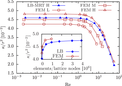
Figure 6: Comparison of the permeability vs. Re obtained using the LB-MRT ($\tau/\Delta t=0.6$ and H) and different resolutions of the FEM grid. The inset shows the resolution dependent permeability for LB (LB-MRT and $\tau/\Delta t=0.6$) and FEM simulations at $\text{Re}\approx 10^{-3}$.

Fig. 6 shows that for both methods the value of the permeability, beyond validity of Darcy’s law, Eq. (1), drops consistently. Darcy’s law is limited to the weak inertia regime, i.e. low Reynolds numbers. To analyze the validity of the simulated data for high Reynolds numbers, we plot ${u_{\rm s}}$ vs. $\langle(\nabla p)_{x_{2}}\rangle$ in Fig. 7 using the H data and $\tau/\Delta t=0.6$ for LB-MRT. For both methods, at small velocity values (small Re), the flow follows Darcy’s prediction (constant slope) and Eq. (1) accurately fits the data. When the velocity increases the measured permeability departs from Darcy’s law and the best possible fit is obtained using Eq. (4), which confirms the existence of a transition regime with cubic velocity dependence. Only for higher velocities the flow enters Forchheimer’s regime and the data can be fitted accurately by Eq. (3). The departure from the different flow regimes is clearly seen in the bottom panel of Fig. 7, where the relative error of the fits is plotted versus Re. It is calculated by

$$\epsilon(w)=\frac{w_{\rm fit}-w_{\rm sim}}{w_{\rm sim}},$$ (20)

where the indices _sim and _fit represent the results obtained by simulation and from the fit, respectively. It can clearly be seen from both datasets that Darcy’s regime holds until $\text{Re}\approx 10^{0}$ and the inertia transition correction expression holds until $\text{Re}\approx 10^{1}$. The Forchheimer’s regime describes the flow for higher Re.

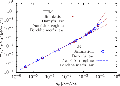
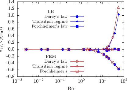
Figure 7: (Top) Fit of the expressions which relate the superficial velocity ${u_{\rm s}}$ and the average pressure gradient $\langle(\nabla p)_{x_{2}}\rangle$ for the porous media flow. (Bottom) Relative error of the fit presented above. The relative error shows that Darcy’s law fits the simulation results for $\text{Re}\lesssim 10^{0}$. Above this value the fit of the expressions given by Eq. (4) is better than the fit with Darcy’s law.

V Conclusions

We presented an analysis of the calculation of the flow in porous media in different flow regimes using the LB method and compared our results to FEM simulations. Special attention has been given to discretization, selection of a collision kernel and choice of parameters. For the LB method a simulation setup combining a constant pressure at the inlet and outlet and an external acceleration acting inside the sample has been proposed in order to reduce compressibility artifacts at high Re. However, at higher Re a substantial number of lattice nodes shows flow velocities beyond 20% of the speed of sound and compressibility effects can clearly be observed. In order to clarify the validity of these results we compare our data to FEM simulations and demonstrate a good quantitative agreement for the full range of Re studied. Furthermore, the data show good agreement with theoretical predictions, demonstrating that the range of Re studied in this work is well accessible for the LB method and that compressibility effects only have a minor influence. The results accurately predict three different flow regimes. These are Darcy’s regime for $\text{Re}\lesssim 10^{0}$, where the average pressure gradient $\langle(\nabla p)_{x_{2}}\rangle$ and the surface velocity ${u_{\rm s}}$ obey a linear relationship. Secondly, a transient regime $10^{0}\lesssim\text{Re}\lesssim 10^{1}$, where the flow is modeled by Darcy’s law plus an inertia correction term represented by a cubic term on ${u_{\rm s}}$, see Eq. (4). Finally, for higher Reynolds numbers ($\text{Re}\gtrsim 10^{1}$) the porous media flow follows Forchheimer’s prediction up to the limit of both simulation methods of Re $\approx$ 30.

VI Acknowledgments

Financial support by STW (STW-MuST program, project number 10120), NWO/STW (VIDI project 10787 and VICI project 10828) and the FOM-Shell IPOG-II IPP is highly acknowledged. Computing time was provided by the Jülich Supercomputing Centre (JSC) and the Scientific Supercomputing Center Karlsruhe (SSCK).

References

- (1) J. Bear. Dynamics of fluids in porous media. Elsevier (New York), 1972.
- (2) K. Moutsopoulos, I. Papaspyros, and V. Tsihrintzis. Experimental investigation of inertial flow processes in porous media. Journal of Hydrology, 374(3-4):242–254, 2009.
- (3) B. Ferréol and D. Rothman. Lattice-Boltzmann simulations of flow through Fontainebleau sandstone. Transp. Porous Media, 20(1-2):3–20, 1995.
- (4) A. Cancelliere, C. Chang, E. Foti, D. H. Rothman, and S. Succi. The permeability of a random medium: Comparison of simulation with theory. Phys. Fluids., 2:2085–2088, 1990.
- (5) Y. H. Qian, D. d’Humières, and P. Lallemand. Lattice BGK models for Navier-Stokes equation. Europhys. Lett., 17(6):479–484, 1992.
- (6) N. Martys and E. Garboczi. Length scales relating the fluid permeability and electrical conductivity in random two-dimensional model porous media. Phys. Rev. B, 46(10):6080–6090, 1992.
- (7) C. Manwart, U. Aaltosalmi, A. Koponen, R. Hilfer, and J. Timonen. Lattice-Boltzmann and finite-difference simulations for the permeability of three-dimensional porous media. Phys. Rev. E, 66(1):016702, 2002.
- (8) S. Succi. The lattice Boltzmann equation for fluid dynamics and beyond. Oxford University Press, 2001.
- (9) E. Aharonov and D. H. Rothman. Non-Newtonian flow (through porous media): a lattice Boltzmann method. Geophys. Research Lett., 20:679, 1993.
- (10) F. Auzerais, J. Dunsmuir, B. Ferreol, N. Martys, J. Olson, T. Ramakrishnan, D. Rothman, and L. Schwartz. Transport in sandstone: a study based on three dimensional microtomography. Geophys. Research Lett., 23(7):705, 1996.
- (11) D. Koch and A. Ladd. Moderate Reynolds number flows through periodic and random arrays of aligned cylinders. J. Fluid Mech., 349:31–66, 1997.
- (12) R. Hill, D. Koch, and A. Ladd. The first effects of fluid inertia on flows in ordered and random arrays of spheres. J. Fluid Mech., 448:213–241, 2001.
- (13) C. Pan, L.-S. Luo, and C. T. Miller. An evaluation of lattice Boltzmann schemes for porous medium flow simulation. Computers & Fluids, 35:898–909, 2006.
- (14) A. Narváez, T. Zauner, F. Raischel, R. Hilfer, and J. Harting. Quantitative analysis of numerical estimates for the permeability of porous media from lattice-Boltzmann simulations. J. Stat. Mech.: Theor. Exp., 2010:P11026, 2010.
- (15) A. Narváez and J. Harting. Evaluation of pressure boundary conditions for permeability calculations using the lattice-Boltzmann method. Adv. in Appl. Math. and Mech., 2:685–700, 2010.
- (16) N. Zabaras and D. Samanta. A stabilized volume-averaging finite element method for flow in porous and binary alloy solidification processes. Int. J. for Num. Meth. in Eng., 60(5):1–38, 2004.
- (17) V. Girault and P. Raviart. Finite elements approximation of the Navier-Stokes equations. Springer Series SCM, 1986.
- (18) F. Thomasset. Implementation of finite element methods for Navier-Stokes equations. Springer-Verlag, New York, 1981.
- (19) T. Tezduyar, M. Behr, and J. Liou. A new strategy for finite element computations involving moving boundaries and interfaces-the deforming spatial-domain/space-time procedure: I. the concept and the preliminary numerical tests. Comput. Meth. Appl. Mech. Eng., 94:339–351, 1992.
- (20) C. Fletcher. Computational Techniques for Fluid Dynamics. Springer, 1991.
- (21) S. Turek. Efficient Solvers for Incompressible Flow Problems: An Algorithmic and Computational Approach. Springer, 1999.
- (22) K. Yazdchi and S. Luding. Towards unified drag laws for inertial flow through fibrous materials. Chemical Engineering Journal, 207:35–48, 2012.
- (23) K. Yazdchi, S. Srivastava and S. Luding. Micro-macro relations for flow through random arrays of cylinders. Composites Part A, 43:2007–2020, 2012.
- (24) H. Darcy. Les fontaines publiques de la ville de Dijon. Dalmont, Paris, 1856.
- (25) F. Dullien. Porous Media: Fluid Transport and Pore Structure. Academic Press, San Diego, 2nd edition, 1992.
- (26) C. Mei and J.-L. Aurialt. The effect of weak inertia on flow through a porous medium. J. Fluid Mech., 222:647–663, 1991.
- (27) G. Massarani. Problemas em sistemas particulados. Ed. Edgard Blucher Ltda, Río de Janeiro, 1984.
- (28) P. Forchheimer. Wasserbewegung durch Boden. Zeit. Ver. Deut. Ing., 45:1781–1788, 1901.
- (29) J. Andrade, U. Costa, M. Almeida, H. Makse, and H. Stanley. Inertial effects on fluid flow through disordered porous media. Phys. Rev. Lett., 82(26):5249–5252, 1999.
- (30) E. Skjetne and J. Auriault. High-velocity laminar and turbulent flow in porous media. Transp. Porous Media, 36:131–147, 1999.
- (31) J.-L. Auriault, C. Geindreau, and L. Orgéas. Upscaling Forchheimer law. Transp. Porous Media, 70:213–229, 2007.
- (32) J.-C. Wodie and T. Levy. Corection non linéaire de la loi de Darcy. C.R. Acad. Sci. Paris, 312:1573–161, 1991.
- (33) M. Firdauss, J.-L. Guermond, and P. Le Quéré. Nonlinear corrections to Darcy’s law at low Reynolds numbers. J. Fluid Mech., 343:331–350, 1997.
- (34) S. Chen, H. Chen, D. Martínez, and W. H. Matthaeus. Lattice Boltzmann model for simulation of magnetohydrodynamics. Phys. Rev. Lett., 67(27):3776–3779, 1991.
- (35) P. L. Bhatnagar, E. P. Gross, and M. Krook. Model for collision processes in gases. I. small amplitude processes in charged and neutral one-component systems. Phys. Rev., 94(3):511–525, 1954.
- (36) J. Sterling and S. Chen. Stability analysis of lattice Boltzmann methods. J. Comp. Phys., 123(1):196–206, 1996.
- (37) Y. H. Qian. Fractional propagation and the elimination of staggered invariants in lattice-BGK models. Int. J. Mod. Phys. C, 8(4):753–761, 1997.
- (38) M. C. Sukop and D. T. Thorne (Jr.). Lattice Boltzmann Modeling, An Introduction for Geoscientists and Engineers. Springer, second edition, 2007.
- (39) D. d’Humières, I. Ginzburg, M. Krafczyk, P. Lallemand, and L.-S. Luo. Multiple-relaxation-time lattice Boltzmann models in three dimensions. Phil. Trans. R. Soc. Lond. A, 360(1792):437–451, 2002.
- (40) P. Lallemand and L.-S. Luo. Theory of the lattice Boltzmann method: dispersion, dissipation, isotropy, Galilean invariance, and stability. Phys. Rev. E, 61(6):6546–6562, 2000.
- (41) I. Ginzburg, F. Verhaeghe, and D. d’Humières. Two-relaxation-time lattice Boltzmann scheme: about parametrization, velocity, pressure and mixed boundary conditions. Comm. Comp. Phys., 3(2):427–478, 2008.
- (42) I. Ginzburg, F. Verhaeghe, and D. d’Humières. Study of simple hydrodynamic solutions with the two-relaxation-times lattice Boltzmann scheme. Comm. Comp. Phys., 3(3):519–581, 2008.
- (43) S. Chapman and T. G. Cowling. The mathematical theory of non-uniform gases. Cambridge University Press, second edition, 1952.
- (44) D. A. Wolf-Gladrow. Lattice-Gas Cellular Automata and lattice Boltzmann models. Springer, 2005.
- (45) D. Kandhai, D.-E. Vidal, A. Hoekstra, H. Hoefsloot, P. Iedema, and P. Sloot. Lattice-Boltzmann and finite element simulations of fluid flow in a smrx static mixer reactor. Int. J. Numer. Meth. Fluids, 31:1019–1033, 1999.
- (46) S. Srivastava, K. Yazdchi, and S. Luding. Meso-scale coupling of FEM/DEM for fluid-particle interactions. In preparation, 2012.
- (47) H. Langtangen, K.-A. Mardal, and R. Winther. Numerical methods for incompressible viscous flow. Adv. in Water Res., 25(8-12):1125–1146, 2002.
- (48) K. Yazdchi, S. Srivastava, and S. Luding. Microstructural effects on the permeability of periodic fibrous porous media. Int. J. of Multiphase Flow, 37(8):956–966, 2011.
- (49) Z. Guo and T. Zhao. Lattice Boltzmann model for incompressible flows through porous media. Phys. Rev. E, 66:036304, 2002.
- (50) Q. Zou and X. He. On pressure and velocity boundary conditions for the lattice Boltzmann BGK model. Phys. Fluids., 9(6):1591–1598, 1997.
- (51) M. Hecht and J. Harting. Implementation of on-site velocity boundary conditions for D3Q19 lattice Boltzmann simulations. J. Stat. Mech.: Theor. Exp., 2010(01):P01018, 2010.