Abstract

Previous results on the non trivial solution of the $\Phi^{4}$-equations of motion for the Green’s functions in the Euclidean  space (of $0\leq r\leq 4$ dimensions) in the Wightman Quantum Field theory framework, are reviewed in the $0-$ dimensional case from the following two aspects:

• (cf.[4]) The structure of the subset $\Phi\subset{\cal B}$ characterized by the bounds signs and “splitting” (factorization properties) is reffined and more explictly described in terms of a new closed subset $\Phi_{0}\subset\Phi\subset{\cal B}$. Using a new norm we establish the local contractivity of the corresponding $\Phi^{4}_{0}$ mapping in the neighborhood of a nontrivial sequence $H_{0}\in\Phi_{0}$.

• A new $\Phi^{4}_{0}$ iteration is defined in the neighborhood of the sequence $H_{0}\in\Phi_{0}$.

  In this paper we present the results of our numerical study, so:

  • a) the stability of $\Phi_{0}$ i.e. the splitting, bounds and sign properties is clearly illustrated in the neighborhood of $H_{0}\in\Phi_{0}$.

  • b) the rapid convergence of this iteration to the fixed point is perfectly realized thanks to the new starting points of the iteration.

1 Introduction

1 A new non perturbative method - the new recent results

Several years ago we started a program for the construction of a non trivial $\Phi^{4}_{4}$ model consistent with the general principles of a Wightman Quantum Field Theory ($Q.F.T.$) [1]. In reference [2] we have introduced a non perturbative method for the construction of a non trivial solution of the system of the $\Phi^{4}$ equations of motion for the Green’s functions, in the Euclidean space of zero, one and two dimensions. In reference [3] we tried to apply an extension of this method to the case of four-(and a fortiori of three-)dimensional Euclidean momentum space.

The general aspects of the method together with its comparison and validity arguments with respect to other non perturbative methods are presented in these previous references, and in particular in the theoretical aspect of this last study [4].

In this paper we present the numerical study of a new $\Phi^{4}_{0}$-Iteration.

We use the zero dimensional analog of the system of equations of motion introduced in the previous papers. The reasons that motivated us for a study in smaller dimensions and not directly in four, were the absence of the difficulties due to the renormalization and the pure combinatorial character of the problem in zero dimensions. Another useful aspect of the zero dimensional case is the fact that it provides a direct way to test numerically the validity of the method.

What are the new developments in the present zero dimensional study:

1. (cf.[4])The “new $\Phi_{0}$ subset is explicitly given in terms of the ”splitting” sequences upper $\left\{\delta_{n,max}(\Lambda)\right\}$ and lower $\left\{\delta_{n,min}(\Lambda)\right\}$ envelops.

2. (cf.[4]) The non triviality and stability of the subset $\Phi_{0}$ under the mapping ${\cal M^{*}}$ is established in terms of the new basic sequences $\left\{\delta_{n,max}(\Lambda)\right\}$, $\left\{\delta_{n,min}(\Lambda)\right\}$ and $\left\{H_{0}\right\}$ The latter is furthermore used for the proof of local contractivity. This proof is simpler in comparison with our previous analogs, due also to the fact that we introduce a new norm on the Banach space $\mathcal{B}$.

3. In the present paper, starting from these particular sequences, $\left\{\delta_{n,max}(\Lambda)\right\}$ and $\left\{\delta_{n,min}(\Lambda)\right\}$, we define a new $\Phi_{0}$-iteration and explore the behavior of the Green’s functions (essentially the $\delta$ functions), at sufficiently large $n$ and reasonable order of this new iteration.

   These last numerical results are convincing, the convergence is rapidly established for different values of $\Lambda$ and the sign and splitting properties (stability+contractivity) give coherent results with respect to our theoretical conclusions.

2 Reminders

In [4] we presented in detail the definitions and results introduced in the previous papers together with the new ones. Let us present only the necessary among them, for the best understanding of our numerical study.

1 The $\Phi^{4}_{0}$  equations of motion the subsets $\Phi_{0}\subset\Phi$ and the new mapping ${\cal M}^{*}$

Definition 1.1 (The $\Phi^{4}_{0}$  equations of motion)

$\forall\ \Lambda\,\in{R}^{+}$

$$H^{2}(\Lambda)=-\Lambda H^{4}(\Lambda)\ \ +1$$ (1.2.1)

and for all $n\geq 3$,

$$H^{n+1}(\Lambda)=\ \ A^{n+1}(\Lambda)+B^{n+1}(\Lambda)+C^{n+1}(\Lambda)$$ (1.2.2)

with:

$$A^{n+1}(\Lambda)=\,-\Lambda H^{n+3}(\Lambda);$$ (1.2.3)

$$B^{n+1}(\Lambda)=\,-3\Lambda\sum_{\varpi_{n}(J)}{n\ !\over j_{1}!j_{2}!}H^{j_{2}+2}(\Lambda)H^{j_{1}+1}(\Lambda);$$ (1.2.4)

$$C^{n+1}(\Lambda)=\,-6\Lambda\sum_{\varpi_{n}(I)}{n\ !\over i_{1}!i_{2}!i_{3}!\ \sigma_{sym}(I)}\prod_{l=1,2,3}H^{i_{l}+1}(\Lambda)$$ (1.2.5)

Here the notation $\varpi_{n}(J)$, means the set of different partitions $(j_{1};j_{2})$ of $n$ such that $j_{1}$ is an odd integer and $j_{1}+j_{2}=n$. Respectively $\varpi_{n}(I)$ is the set of triplets of odd numbers-different ordered partitions $(i_{1};i_{2};i_{3})$ of $n$ with $i_{1}\geq i_{2}\geq i_{3}$.

The symmetry-integer $\sigma_{sym}(I)$ is defined by:

$$\sigma_{sym}(I)=\left\{\matrix{\hfill 3!&if&i_{1}=i_{2}=i_{3}\cr\hfill 1&if&i_{1}\neq i_{2}\neq i_{3}\neq i_{1}\cr\hfill&2&otherwise\cr}\right\}$$ (1.2.6)

2 The vector space ${\cal B}$

Definition 1.2

We introduce the vector space ${\cal B}$ of the sequences $H=\{H^{n+1}\}_{n=2k+1;k\in{N}}$ by the following: The functions $H^{n+1}(\Lambda)$ belong to the space $C^{\infty}({R}^{+})$ of continuously differentiable numerical functions of the variable $\Lambda\in{R}^{+}$ (which physically represents the coupling constant).

Moreover, there exists a universal (independent of n and of $\Lambda$) positive constant $K_{0}$, such that the following uniform bounds are verified:

$$\forall\ n=2k+1,k\in{N}$$

$$|H^{n+1}(\Lambda)|\leq n\ !(K_{0})^{n}\qquad\forall\,\Lambda\in{R}^{+}$$ (1.2.7)

We suppose that the system of equations under consideration, concerns always (following our introduction and the previous definition) the sequences of Euclidean connected and amputated with respect to the free propagators Green’s functions (the Schwinger functions). and that these sequences denoted by $H=\{H^{n+1}\}_{n=2k+1\;,k\in{N}}$ belong to the above space ${\cal B}_{c}$.

3 The splitting sequences and the subsets $\Phi_{0}\subset\Phi\subset{\cal B}$

Definition 1.3

We first introduce the class ${\cal D}$ of sequences

$$\delta=\{\delta_{n}(\Lambda)\}_{n=2k+1;k\in{N}}\in{\cal B},$$

such that they verify the bounds $(2.1.1)$ in the following simpler form:

$$|\delta_{n}(\Lambda)|\leq\,K_{0},$$ (1.2.8)

$$\forall\,n=2k+1;\ k\in{N}$$

Definition 1.4

splitting and signs-$\Phi\subset{\cal B}$

We shall say that a sequence $H\in{\cal B}$ belongs to the subset $\Phi\subset{\cal B}$ if there exists an increased associated sequence of positive and bounded functions on ${R}^{+}$,

$$\delta=\{\delta_{n}(\Lambda)\}_{n=2k+1;k\in{N}}\in{\cal D},$$

such that the following “splitting” (or factorization) and sign properties are verified:

$$\forall\Lambda\in{R}^{+}$$

$\Phi.1$

$$H^{2}(\Lambda)=1+\Lambda\delta_{1}(\Lambda)\,\hbox{ with:}\,\,\mathrel{\mathop{\kern 0.0pt\lim}\limits_{\Lambda\rightarrow 0}}\delta_{1}(\Lambda)=0$$ (1.2.9)

$\Phi.2$

$$H^{4}(\Lambda)=-\delta_{3}(\Lambda)[H^{2}(\Lambda)]^{3},\,\hbox{ with:}\,\,\delta_{3}(\Lambda)\leq 6\Lambda,\ \mathrel{\mathop{\kern 0.0pt\lim}\limits_{\Lambda\rightarrow 0}}{\delta_{3}(\Lambda)\over\Lambda}=6$$ (1.2.10)

$\Phi.3$

$$\forall n\geq 5\qquad H^{n+1}(\Lambda)={\displaystyle\delta_{n}(\Lambda)C^{n+1}\over\displaystyle 3\Lambda n(n-1)},\ \hbox{ with :}\,\ \mathrel{\mathop{\kern 0.0pt\lim}\limits_{\Lambda\rightarrow 0}}{\displaystyle\delta_{n}(\Lambda)\over\displaystyle\Lambda}=3n(n-1)$$ (1.2.11)

$\Phi.4$

$\forall\,\,n=2k+1$  with  $k\in{N}^{*},\,\exists$ positive continuous functions of $\Lambda$,

$$\delta_{n,max}(\Lambda),\ \delta_{n,min}(\Lambda)$$

(uniform bounds independent on $H$), $\delta_{max}^{\infty}$, $\delta_{\infty}$ (uniform limit and bound at infinity), such that:

$$\delta_{n,max}(\Lambda)\ >\ \delta_{n,min}(\Lambda)$$ (1.2.12)

$$\delta_{n,min}(\Lambda)\leq\delta_{n}(\Lambda)\leq\delta_{n,max}(\Lambda)$$ (1.2.13)

$$\mathrel{\mathop{\kern 0.0pt\lim}\limits_{n\rightarrow\infty}}\delta_{n,max}\leq\delta_{max}^{\infty}(\Lambda)\leq\delta_{\infty}$$ (1.2.14)

Definition 1.5

$$\delta_{3,max}(\Lambda)=6\Lambda;\qquad\delta_{3,min}(\Lambda)={6\Lambda\over 1+9\Lambda(1+6\Lambda^{2})}$$ (1.2.15)

and  $\forall\,\,n\geq 5$

$$\delta_{n,max}(\Lambda)\,={3\Lambda\ n(n-1)\over 1+3\Lambda\ n(n-1)d_{0}}$$ (1.2.16)

here we put $d_{0}=0.001$

$$\delta_{n,min}(\Lambda)\,={3\Lambda\ n(n-1)\over 1+3\Lambda\ n\ (n-1)}$$ (1.2.17)

Definition 1.6

By using $\{\delta_{n,max}(\Lambda)\}_{n=2k+1;k\in{N}}$  and  $\{\delta_{n,min}(\Lambda)\}_{n=2k+1;k\in{N}}$ introduced before we define the following sequences:

$$\{H^{n+1}_{max}\}_{n=2k+1;k\in{N}}\in{\cal B}\,\hbox{\emph{and}}\,\{H^{n+1}_{min}\}_{n=2k+1;k\in{N}}\,\in{\cal B}$$

$$H^{2}_{max}(\Lambda)=(1+6\Lambda^{2})^{2};\ \qquad H^{2}_{min}=1$$ (1.2.18)

$$H^{4}_{max}(\Lambda)=-6\Lambda[H^{2}_{max}]^{3};\ \ H^{4}_{min}(\Lambda)=-\delta_{3,min}(\Lambda)$$ (1.2.19)

and recurrently for every $n\geq 5$ :

$$H^{n+1}_{max}={\delta_{n,max}(\Lambda)C^{n+1}_{max}\over 3\Lambda\ n(n-1)}$$ (1.2.20)

$$H^{n+1}_{min}(\Lambda)={\delta_{n,min}(\Lambda)C^{n+1}_{min}\over 3\Lambda\ n(n-1)}$$ (1.2.21)

Definition 1.7

The subset $\Phi_{0}$

Taking into account the sequences of the previous definition   we introduce the following subset $\Phi_{0}\subset\Phi$:

$$\Phi_{0}=\left\{H\in\Phi:|H^{n+1}_{min}|\ \leq|H^{n+1}|\leq|H^{n+1}_{max}|,\quad\forall n=2k+1,\ k\in\ {N}\right\}$$ (1.2.22)

Using the previous sequences we defined in [4] the “fundamental sequence”.

Definition 1.8

$$H^{2}_{0}(\Lambda)=1-\Lambda H^{4}_{min}\ \ \$$ (1.2.23)

$$H^{4}_{0}(\Lambda)=-\delta_{3,0}(\Lambda)[H^{2}_{0}]^{3}\quad\hbox{with}\quad\delta_{3,0}(\Lambda)=\displaystyle{\frac{6\Lambda}{1+9\Lambda-\displaystyle{\frac{\Lambda|H^{6}_{min}|}{|H^{4}_{min}|}}}}$$ (1.2.24)

and for every $n\geq 5$

$$H^{n+1}_{0}(\Lambda)={\delta_{n,0}(\Lambda)C^{n+1}_{0}(\Lambda)\over 3\Lambda n(n-1)};$$ (1.2.25)

with:

$$C^{n+1}_{0}(\Lambda)=-6\Lambda\sum_{\varpi_{n}(I)}{n\ !\over i_{1}!i_{2}!i_{3}!\ \sigma_{sym}(I)}\prod_{l=1,2,3}H^{i_{l}+1}_{0}(\Lambda);$$ (1.2.26)

$$\delta_{n,0}(\Lambda)=\frac{3\Lambda n(n-1)}{1+D_{n}(H_{(min)})}$$ (1.2.27)

and

$$D_{n}(H_{(min)})=\displaystyle{\frac{|B^{n+1}_{min}|-|A^{n+1}_{min}|}{|H^{n+1}_{max}|}}$$ (1.2.28)

and proved,

Proposition 1.1

(the non triviality)

The set of sequences $\Phi$ given by the definition 1.4 is a nontrivial subset of the space ${\cal B}$.

Then, we introduced

Definition 1.9

The new mapping ${\cal M^{*}}$

$${\cal M^{*}}:\,\Phi\stackrel{{\scriptstyle\cal M^{*}}}{{\longrightarrow}}{\cal B}$$

$$H^{2^{\prime}}(\Lambda)=1+\Lambda\delta_{1}^{{}^{\prime}}(\Lambda)\qquad\hbox{with}\qquad\delta_{1}^{{}^{\prime}}(\Lambda)=-H^{4}(\Lambda)$$ (1.2.29)

$$H^{4^{\prime}}(\Lambda)=-\delta_{3}^{\prime}(\Lambda)[H^{2^{\prime}}]^{3}\quad\hbox{with}\quad\delta_{3}^{{}^{\prime}}(\Lambda)=6\Lambda[1+6\Lambda H^{2}(3/2-\frac{|H^{6}|}{6|H^{4}||H^{2}|})]^{-1}$$ (1.2.30)

and for every $n\geq 5$

$$H^{n+1^{\prime}}(\Lambda)={\delta_{n}^{{}^{\prime}}(\Lambda)C^{n+1^{\prime}}(\Lambda)\over 3\Lambda n(n-1)};$$ (1.2.31)

and:

$$\delta_{n}^{{}^{\prime}}(\Lambda)=\frac{3\Lambda n(n-1)}{1+D_{n}(H)}$$ (1.2.32)

with

$$D_{n}(H)={|B^{n+1}|-|A^{n+1}|\over|H^{n+1}|}$$ (1.2.33)

and proved:

Theorem 1.1

The stability of the subset $\Phi_{0}$

If $H\in\Phi$; then ${\cal M^{*}}(H)\subset\Phi$ under the condition:

$$0<\Lambda\leq 0.05$$

Furthermore (always in [4]), we constructed a Banach space ${\cal B}_{c}\subset{\cal B}$ by introducing the following norm ${\cal N}$:

Definition 1.10

$$\begin{array}[]{l}{\cal N}:\ {\cal B}\rightarrow{R}^{+}\\ \ \ \ \ H\mapsto\|H\|\ \ \hbox{with:}\ \ \|H\|=\{\displaystyle{\sup_{\Lambda;n}}\displaystyle{\frac{|H^{n+1}|}{M_{n}}\}}\end{array}$$ (1.2.34)

Here $\forall\ \ \Lambda\in{R}^{+}$:

$$M_{1}(\Lambda)=H^{2}_{max}=(1+6\Lambda^{2})^{2};\quad M_{3}(\Lambda)=\,\delta_{3max}(M_{1})^{3};\ \$$ (1.2.35)

and for every $n\geq 5$

$$\begin{array}[]{l}M_{n}(\Lambda)=\ n(n-1)\delta_{nmax}M_{n-2}(M_{1})^{2}\end{array}$$ (1.2.36)

The function ${\cal N}$ above defines a finite norm inside a non empty subspace ${\cal B}_{c}$ of ${\cal B}$. This subspace ${\cal B}_{c}$ obviously contains $\Phi_{c}$ and is a Banach space with respect to the ${\cal N}$- topology.

Using the above definition of the norm we introduced a ball-neighborhood $S_{\rho}(H_{0})$ of the fundamental sequence and by theorem 1.2, we have established the local contractivity of ${\cal M^{*}}$ inside it by the following:

Theorem 1.2

the local contractivity of the mapping ${\cal M^{*}}$  in $S_{\rho}(H_{0})\ \subset\Phi_{0}$

There exists a finite positive constant $\Lambda^{*}(\approx 0.45)$ such that the mapping ${\cal M^{*}}$ is locally contractive in $S_{\rho}(H_{0})$ consequently there exiists a unique non trivial solution of the $\Phi_{0}^{4}$ equations of motion in the neihbourhood $S_{\rho}(H_{0})\ \subset\Phi_{0}$ of the fundamental sequence $H_{0}$.

2 The numerical study

1 The different aspects of the analysis

We have studied three different aspects of our study, consequently we have obtained three sets of figures, that we describe in detail in what follows.

The general conclusion of this numerical experience appears clearly the same in all three sets.

We notice that the first three orders of the iteration of $\delta_{n,max}$ and $\delta_{n,max}$ yield different curves which come closer to each other till the fourth order iteration. Beyond, i.e. for $5^{th}$ and $6^{th}$ order, we observe a perfect coincidence of $\delta_{n,max}$ and $\delta_{n,min}$.

So, when the value of $\Lambda$ lies in $[0.001,\ 0.1]$, the neighborhood where lies the fixed point of the contractive mapping is manifestly around the $\{H_{0}\}$ sequence, (almost first order iteration of $\{\delta_{n,min}\}$ sequence). This fact is enhanced by the following observation:

For a given value of $\Lambda$ we remark that the sequence $\{\delta_{n,max}\}$ decreases during the iteration procedure (resp the sequence $\{\delta_{n,min}\}$ increases). The two sets are almost the same up to the fourth iteration. We notice that the decreasing rate of $\{\delta_{n,max}\}$ is more important than the increasing rate of $\{\delta_{n,min}\}$, and this again underlines the fact that the $\{H_{0}\}$ neighborhood is the best for the local contractivity.

This result is more satisfactory (from the point of view of the bound of $\Lambda$) in comparison with the theoretical proof of the validity of the contractivity criteriun at $\Lambda\leq 0.05$.

1 First set of figures

The first set of figures displays the convergence proof of the mapping for different values of $\Lambda$, using as stating points both $\delta_{n,max}$ and $\delta_{n,min}$. This set represents the results of twenty iterations of the mapping for different values of $\Lambda$
(i.e $\Lambda\in\{0.001,\ 0.01,\ 0.03,\ 0.05,\ 0.075,\ 0.1\}$) at $n$ fixed. We have chosen ten different values of $n$:

$$n=7,\ 9,\ 11,\ 13,\ 15,\ 17,\ 19,\ 21,\ 23,\ 25.$$

The stability of the values is already attained at the tenth iteration for all values of $n$.

2 Second set of figures

The second set displays the convergence of the mapping up to the sixth iteration, for different values of $\Lambda$.

3 Third set

The third set of figures displays the summary of the previous configuration, for the sixth iteration.

This figure represents the results of the mapping of $\delta_{n}$ functions, for

$$n=7,\ 9,\ 11,\ 13,\ 15,\ 17,\ 19,\ 21,\ 23,\ 25.$$

for different values of $\Lambda$
(i.e $\Lambda\in\{0.001,\ 0.01,\ 0.03,\ 0.05,\ 0.075,\ 0.1\}$) and for all $20$ iterations.

The figure illustrates clearly the convergence of the iteration to the fixed point. We remark also that the convergence is more rapid for sufficiently small values of $\Lambda$ (and even for bigger than the critical point $0.45$, due to the small values of $n$).

Our experience shows that the stability is impossible, for example $n=1000$, when $\Lambda$ becomes bigger than $0.05$.

This figure represents the results of the mapping of $\delta_{n}$ functions as surfaces of $n$ and $\nu$ for fixed $\Lambda$ (at the six different values).

We remark in this figure that:

• For small values of $\Lambda$ ($\Lambda\leq 0.001$), the ”decrease” properties of $\delta_{n}$’s are not apparent.

• For the intermediate values (”good values”) of $\Lambda$, the surfaces show the expected concavity as far as $\nu$ (iteration number) increases.

• For large values of $\Lambda$ (bigger than the critical value $\sim 0.045$), we observe a rapid increasing surface (because we are far from the stability and contractivity criteria).

3 The figures

1. 

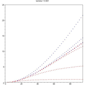
   Figure 1: $1^{rst}$ set: Convergence up to $\nu=6$ with $\Lambda=0.001$ starting from $\delta_{n,max}$ and $\delta_{n,min}$

2. 

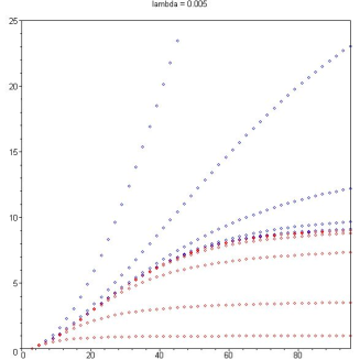
   Figure 2: $1^{rst}$ set: Convergence up to $\nu=6$ with $\Lambda=0.0005$ starting from $\delta_{n,max}$ and $\delta_{n,min}$

3. 

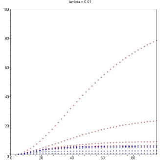
   Figure 3: $1^{rst}$ set: Convergence up to $\nu=6$ with $\Lambda=0.01$ starting from $\delta_{n,max}$ and $\delta_{n,min}$

4. 

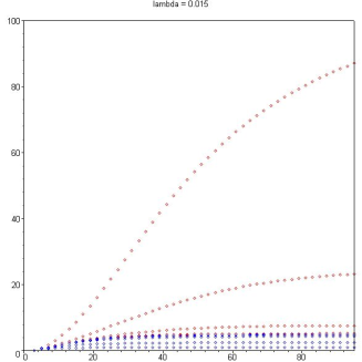
   Figure 4: $1^{rst}$ set: Convergence up to $\nu=6$ with $\Lambda=0.015$ starting from $\delta_{n,max}$ and $\delta_{n,min}$

5. 

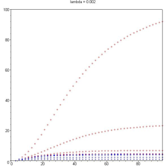
   Figure 5: $1^{rst}$ set: Convergence up to $\nu=6$ with $\Lambda=0.02$ starting from $\delta_{n,max}$ and $\delta_{n,min}$

6. 

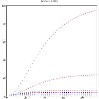
   Figure 6: $1^{rst}$ set: Convergence up to $\nu=6$ with $\Lambda=0.025$ starting from $\delta_{n,max}$ and $\delta_{n,min}$

7. 

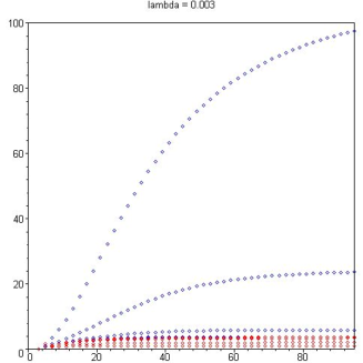
   Figure 7: $1^{rst}$ set: Convergence up to $\nu=6$ with $\Lambda=0.03$ starting from $\delta_{n,max}$ and $\delta_{n,min}$

8. 

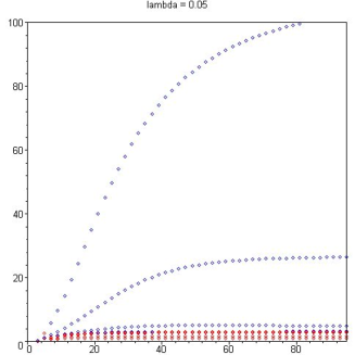
   Figure 8: $1^{rst}$ set: Convergence up to $\nu=6$ with $\Lambda=0.05$ starting from $\delta_{n,max}$ and $\delta_{n,min}$

9. 

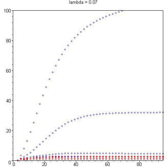
   Figure 9: $1^{rst}$ set: Convergence up to $\nu=6$ with $\Lambda=0.07$ starting from $\delta_{n,max}$ and $\delta_{n,min}$

10. 

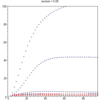
    Figure 10: $1^{rst}$ set: Convergence up to $\nu=6$ with $\Lambda=0.09$ starting from $\delta_{n,max}$ and $\delta_{n,min}$

11. 

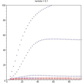
    Figure 11: $1^{rst}$ set: Convergence up to $\nu=6$ with $\Lambda=0.1$ starting from $\delta_{n,max}$ and $\delta_{n,min}$

12. 

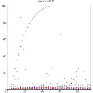
    Figure 12: $1^{rst}$ set: Divergence up to $\nu=6$ with $\Lambda=0.15$ starting from $\delta_{n,max}$ and $\delta_{n,min}$

13. 

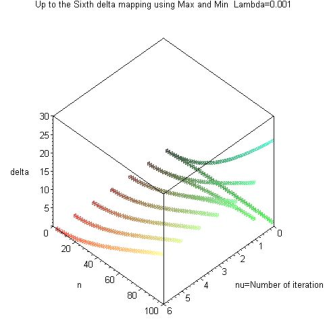
    Figure 13: $2^{nd}$ set: Convergence up to $\nu=6$ with $\Lambda=0.001$ starting from $\delta_{n,max}$ and $\delta_{n,min}$

14. 

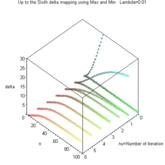
    Figure 14: $2^{nd}$ set: Convergence up to $\nu=6$ with $\Lambda=0.01$, starting from $\delta_{n,max}$ and $\delta_{n,min}$

15. 

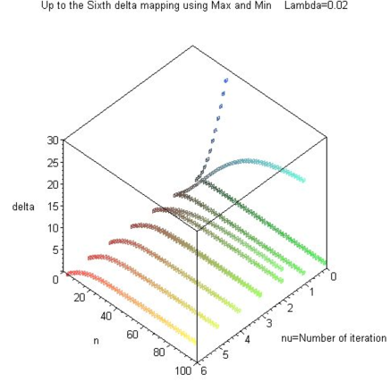
    Figure 15: $2^{nd}$ set: Convergence up to $\nu=6$ with $\Lambda=0.02$, starting from $\delta_{n,max}$ and $\delta_{n,min}$

16. 

    Figure 16: $2^{nd}$ set: Convergence up to $\nu=6$ with $\Lambda=0.03$, starting from $\delta_{n,max}$ and $\delta_{n,min}$

17. 

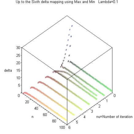
    Figure 17: $2^{nd}$ set: Convergence up to $\nu=6$ with $\Lambda=0.1$, starting from $\delta_{n,max}$ and $\delta_{n,min}$

18. 

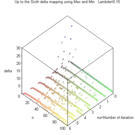
    Figure 18: $2^{nd}$ set: Divergence (up to $\nu=6$) with $\Lambda=0.15$, starting from $\delta_{n,max}$ and $\delta_{n,min}$

    

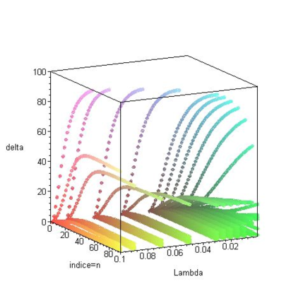
    Figure 19: $3^{d}$ set: Summary up to the sixth iteration for $\Lambda$ from $0.001$ to $0.01$

    

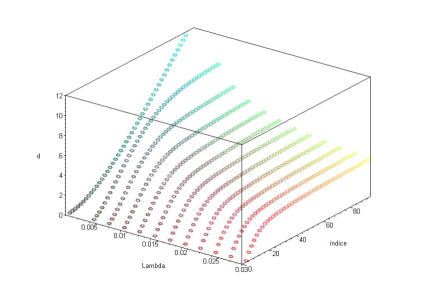
    Figure 20: $3^{d}$ set: Summary of the six iterations for $\Lambda$ from $0.001$ to $0.03$