Hyperbolic Structure and Stickiness Effect: A case of a 2D Area-Preserving Twist Mapping

Abstract

The stickiness effect suffered by chaotic orbits diffusing in the phase space of a dynamical system is studied in this paper. Previous works have shown that the hyperbolic structures in the phase space play an essential role in causing the stickiness effect. We present in this paper the relationship between the stickiness effect and the geometric property of hyperbolic structures. Using a two-dimensional area-preserving twist mapping as the model, we develop the numerical algorithms for computing the positions of the hyperbolic periodic orbits and for calculating the angle between the stable and unstable manifolds of the hyperbolic periodic orbit. We show how the stickiness effect and the orbital diffusion speed are related to the angle.

Received October 20, 2010; accepted March 3, 2011; published online February 8, 2012

 

stickiness effect, hyperbolic structure, stable and unstable manifolds

1 Introduction

In a $2n$-dimensional phase space of a dynamical system, given long enough time, a chaotic orbit would visit any place in the connected chaotic region, owning to the ergodicity property. Only those regions surrounded by the $(2n-1)-$dimensional invariant surface (curve) are forbidden to the chaotic orbit. During its diffusion in the phase space, a chaotic orbit generally spends much longer time wandering near the regular regions than elsewhere. This phenomenon is called the “stickiness effect” [1, 2], and it causes the anomalous chaotic transport [3–7]. The phase spaces of most physically realistic systems consist of chaotic and regular components, thus the stickiness effect is a generic phenomenon. Especially, in those nearly integrable systems such as the Solar System [8], the slow diffusion is a key point to understand the stabilities of those systems. As a matter of fact, the diffusion (transport) in the phase space is a very important issue in many areas, with interests not only of the general theory of dynamical system but also of direct applications in physics and astrophysics. For example, this type of dynamics has implications in the tokamak fusion [e.g. 9], turbulence [e.g. 10], plasma physics [e.g. 11], semiconductor superlattices [e.g. 12], quantum chaos [e.g. 13], galaxy dynamics [e.g. 14], etc.

The stickiness effect was first recognized in the close vicinity of the KAM tori [1, 2], but it seemingly may arise from many other structures in the phase space, including the island chains, the cantori, the hyperbolic structures, and the asymptotic curves of the unstable periodic orbits [see e.g. 2, 15–24]. We have shown in our previous papers [25, 26] that the hyperbolic invariant sets play a critical role in causing the stickiness effects. Using models of both 2-dimensional (2D) mapping [25] and 3-dimensional (3D) mapping [26], we have shown that a diffusing orbit is generally “stuck” by the hyperbolic structures in the 2D or 3D phase space. There seems to be an essential relation between the hyperbolic structures and the stickiness effects.

Many studies on the stickiness effect focused on the diffusion behaviors in the phase space, by illustrating what structures may have stickiness effects [see e.g. 16, 20, 21, 23], or by describing the rules of diffusion in different regimes [e.g. 8, 16, 17, 27]. As for the geometric details of the structures causing the stickiness effect, Contopoulos and Harsoula [23] calculated the sizes of gaps in a cantorus being crossed by an orbit and relate the size of the “maximum gap” with the diffusion time.

Obviously the diffusion orbits have to pass through the “gaps” when crossing a cantorus. In a 2D phase space, the hyperbolic periodic orbits are included in cantori and island chains. When an orbit crosses these structures on its diffusion route, it approaches from one side to the hyperbolic periodic point along the stable manifold and then it may leave from the other side along the unstable manifold. Therefore, the geometric features of the phase space influence strongly the characteristic of diffusing trajectories. In this paper, we try to explore the geometric structures around the cantori, in particular, we study the angle between the stable and unstable manifolds around the cantori.

To do this, it is necessary to know first the exact positions of the cantori and the directions of the stable and unstable manifolds mentioned above. But, since a cantorus is unstable, it’s difficult to locate its position precisely. Consequently, the directions of the manifolds can hardly be determined accurately. Using a 2D mapping model, we will introduce the methods for calculating such positions and directions with high precision, then calculate the angle between the directions of the stable and unstable manifolds, and finally we will study the relation between the diffusion speed and the sizes of the angles. We find that the diffusion speed increases when the size of angles increases.

The mapping model used in this paper is obtained by a modification to the so called “standard mapping”. Contrary to the standard mapping whose “twist” depends linearly on the action-variable, our mapping model has a nonlinear twist. Such a nonlinearity in twist is often seen in physics [28].

The paper is organized as follows. In Section 2, we introduce the mapping model. We show in Section 3 how to locate the precise positions of hyperbolic periodic orbits in the phase space and present the method of calculating the angle between stable and unstable manifolds. The characteristic angles of the hyperbolic structures in different regions and the diffusion speeds of orbits diffusing across these regions are compared in Section 4. And finally we make the conclusions in Section 5.

2 Mapping Model

Generally a mapping is much easier to handle than a set of differential equations (e.g. a Hamiltonian system) as a dynamical system. Thus we use a mapping model in this paper as usual.

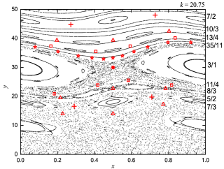
Figure 1: The phase space of the mapping (Eq. (6)) with the parameter $k=20.75$. Some hyperbolic periodic orbits (fixed points) are located and plotted. To present a clean appearance, the period-two orbits are indicated by crosses, and the period-3, 4 orbits are indicated by triangles and squares, respectively. The 3/1 and the 35/11 periodic orbits are indicated by a solid dot and stars. The rotation number of the orbits are labeled on the right side.

2.1 The mapping

We begin from the well-known standard mapping [29]:

$$\left\{\begin{array}[]{l}\tilde{x}^{\prime}=\tilde{x}-\tilde{y}^{\prime},\\ \tilde{y}^{\prime}=\tilde{y}+\frac{k}{2{\uppi}}\sin(2{\uppi}\tilde{x}),\end{array}\right.$$ (1)

which can be generated from a generating function

$$\tilde{S}=\frac{1}{2}(\tilde{x}-\tilde{x}^{\prime})^{2}+\frac{k}{4{\uppi}^{2}}\cos(2{\uppi}\tilde{x}),$$ (2)

through equations

$$\left\{\begin{array}[]{l}\tilde{y}=\tilde{S}_{\tilde{x}}=\frac{\partial\tilde{S}}{\partial\tilde{x}}=\tilde{x}-\tilde{x}^{\prime}-\frac{k}{2{\uppi}}\sin(2{\uppi}\tilde{x}),\\ \tilde{y}^{\prime}=-\tilde{S}_{\tilde{x}^{\prime}}=-\frac{\partial\tilde{S}}{\partial\tilde{x}^{\prime}}=\tilde{x}-\tilde{x}^{\prime}.\end{array}\right.$$ (3)

Here we modify the generating function by adding an extra high-order term $\frac{1}{4}(x-x^{\prime})^{4}$,

$$S=\frac{1}{2}(x-x^{\prime})^{2}+\frac{1}{4}(x-x^{\prime})^{4}+\frac{k}{4{\uppi}^{2}}\cos(2{\uppi}x),$$ (4)

thus the corresponding area-preserving mapping is given by

$$\left\{\begin{array}[]{l}y=S_{x}=(x-x^{\prime})+(x-x^{\prime})^{3}-\frac{k}{2{\uppi}}\sin(2{\uppi}x),\\ y^{\prime}=-S_{x^{\prime}}=(x-x^{\prime})+(x-x^{\prime})^{3}.\end{array}\right.$$ (5)

Explicitly, the mapping reads

$$\left\{\begin{array}[]{l}x^{\prime}=x-\sqrt[3]{\frac{y^{\prime}}{2}+\sqrt{\frac{y^{\prime 2}}{4}+\frac{1}{27}}}-\sqrt[3]{\frac{y^{\prime}}{2}-\sqrt{\frac{y^{\prime 2}}{4}+\frac{1}{27}}}\hskip 14.22636pt{\rm mod}(1),\\ y^{\prime}=y+\frac{k}{2{\uppi}}\sin(2{\uppi}x).\end{array}\right.$$ (6)

This mapping is defined on the cylinder $0\leq x\leq 1,-\infty<y<+\infty$, and $k$ is the only one perturbation parameter. As in the standard mapping, the $y$ in this mapping is the action variable, and the $x$ is the angle variable that can be performed the modulus over 1. As usual, in this paper, by “diffusion” we mean the drifting of the action variable $y$ in the phase space. In the study by Cheng and Sun [30], it was shown that for any given $k$, this mapping behaves chaotically around $|y|<M$ (where $M>0$), and the KAM curves exist at large $|y|$. When $k$ is small, the phase space of the mapping is mainly full of (horizontal) invariant tori. As $k$ increases, the KAM tori break, first at low $|y|$ value, and chaos sets in. The area occupied mainly by chaotic orbits extends outward from the region around $y=0$. We show in Fig. 1 the phase space when $k=20.75$. Note that the negative $y$ half of the phase space is symmetric to the positive half that has been shown in Fig. 1.

Figure 2: The rotation number of the mapping ($k=20.75$). Open squares show the change of rotation number along the vertical line $x=0.0$, while the crosses are for the line $x=0.5$.

The mapping is an area-preserving monotone twist mapping, thus along a vertical line in the phase space the rotation number increases monotonically. The rotation numbers along two vertical lines are computed and shown in Fig. 2. Clearly, the scattering distribution in the lower left corner of Fig. 2 is a reflection of the chaotic motion at low $y$ value in the phase space. The “plateaus” in both cases arise from the fact that the vertical lines cross stable islands, on which the rotation numbers are constants.

2.2 The orbital diffusion in the phase space

Any chaotic orbit in the connected chaotic sea of the phase space will wander ergodically as time tends to infinity. But, it is known that an orbit spends much longer time in some specific regions than elsewhere, e.g., the close vicinity around an embedded island, the region where a KAM torus had newly broken, the region occupied by hyperbolic structures, etc. This is called the stickiness effect, as we mentioned above.

To show a typical orbital diffusion process and the stickiness effect, we arbitrarily select an initial point $(x_{0},y_{0})=(0.49,29.0)$ not far away from the regular region in the upper part of Fig. 1, and follow its evolution. The diffusion of this orbit is shown in Fig. 3.

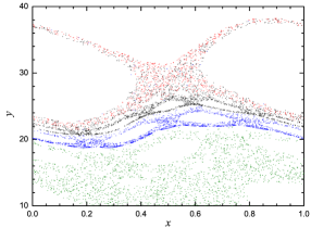
Figure 3: The diffusion process of an arbitrary orbit starting from $(x_{0},y_{0})=(0.49,29.0)$. The red, black and blue points represent its trajectories during the time (iteration number $n$) intervals of $(1,9\times 10^{4}),(9\times 10^{4},4.5\times 10^{7})$ and $(4.5\times 10^{7},7\times 10^{7})$. After $\sim 6\times 10^{9}$ iterations, it finally crosses the compact partial barrier (see text), which makes the bottom boundary of blue points, and enters the open chaotic sea around $y=0$ (green dots).

On its route of downward diffusion, the orbit meets some structures that play the role of obstacles. As shown in Fig. 3, the orbit wanders around the 3/1 fixed point and the corresponding island (see Fig. 1 to find the positions of island-chains of different rotation numbers) at beginning (red points trajectory). This island does not show a significant stickiness effect, but the orbit spends much longer time in next stage around the vicinity of the 11/4 island-chain (black dots in Fig. 3). After that, it was obstructed by another barrier, which prevents the orbit from further diffusing downward, and only after pretty long time, the orbit can reach the 8/3 island chain (blue dots). Then, the diffusion was strongly obstructed by a partial barrier below the 8/3 island chain. Only after $\sim 6\times 10^{9}$ iterations, the orbit can cross this “compact” barrier and enter finally the open chaotic sea around $y=0$ (green dots). In fact, the rotation number around this compact partial barrier is around 2.6 (see Fig. 2). We suspect that this difficult-to-cross barrier is the remnant of the last and most robust KAM torus that has the “golden rate” rotation number. And this will be verified in next section.

One thing we would like to address here is that the orbit may cross an obstacle in both forward and backward directions, that is, an orbit may cross the same partial barrier several times back and forth. After leaving a region, it may re-enter the region again some time later. That’s why we see the black dots and red dots are mixed around the 3/1 island in Fig. 3.

Typically, an orbit starting above the lowest and difficult-to-cross barrier mentioned above would spend time as long as several $10^{9}$ iterations before crossing it. In attempt to show some details of this barrier, we plot in Fig. 4 three orbits starting close to it, from initial points $P_{1}=(0.509,21.667),P_{2}=(0.509,21.672)$ and $P_{3}=(0.509,21.677)$ respectively. These initial points are indicated by three crosses in Fig. 4b. From this magnified picture, we realize that $P_{3}$ (black) is on an island-chain with a high period number. The orbit initialized at $P_{2}$ (red) finally diffuses upward after several $10^{9}$ iterations, while the one from $P_{1}$ (blue) diffuses downward. There is a mixed region where we can find both red and blue dots, indicating clearly the existence of the difficult-to-cross partial barrier.

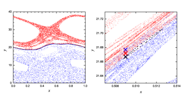
Figure 4: The most sticky region. Three initial points (crosses) and the corresponding trajectories (dots) are shown in black, red and blue.

3 Angle between stable and unstable manifolds

The diffusion of an orbit is through the hyperbolic structures between the islands in an island-chain, which is in fact the relic of the KAM tori if the rotation number in this position does not satisfy the Diophantine condition [31]. On the other hand, if the rotation number is irrational enough, there would be a cantorus left after the breaking of the KAM torus. And an orbit’s diffusion is through the gaps in the cantorus. But the cantorus itself is composed of hyperbolic points and in the gaps exist the hyperbolic structures.

In this paper, we will describe the geometric property of the hyperbolic structures and find out how this property affects the diffusion speed. We will show that the diffusion speed is determined by the angle between the stable and unstable manifolds of the hyperbolic structure. In this section, we introduce the algorithm for calculating the angle between the stable and unstable manifolds of a hyperbolic structure.

3.1 The locations of hyperbolic periodic points

Usually a recursive algorithm is employed to compute the locations of periodic orbits. But it does not work for the hyperbolic ones because these orbits are unstable. Fortunately, the hyperbolic periodic orbits we are looking for in this model are of minimal action, therefore the gradient algorithm could be used to find these orbits. The existence of these minimal periodic orbits is guaranteed by Aubry-Mather theory [32].

Suppose $x_{0},x_{1},\cdots,x_{p-1},x_{p}$ are the variables in the configuration space of a minimal periodic orbit of rotation number $q/p$, with $q$ and $p$ being coprime integers. Obviously, $x_{p}=x_{0}+q$. The action functional $f$ corresponding to this periodic orbit is:

$$f(x_{0},x_{1},\cdots,x_{p-1})=S(x_{0},x_{1})+S(x_{1},x_{2})+\cdots+S(x_{p-1},x_{p}),$$ (7)

where $S$ is the generating function (Eq. (4)). Then the minimal periodic configuration $(x_{0},x_{1},\cdots,x_{p-1},x_{p})$ is the minimum of $f$. Therefore, a periodic orbit of rotation number $q/p$ can be found by locating the minimum of the above mentioned functional. To find the minimum, we may use the gradient algorithm.

Consider the following differential equation:

$$\dot{\Xi}=-\nabla f(\Xi)$$ (8)

where $\Xi=(\xi_{0},\xi_{1},\cdots,\xi_{p-1})^{T}$ is a column vector and the dot over it indicates time derivative. A trajectory defined by this differential equation converges to a minimum of the functional $f$ as $t\rightarrow\infty$. Thus, a minimal periodic orbit can be obtained through integrating this differential equation.

Specifically in our model, since

$$S_{x_{k}}(x_{k-1},x_{k})=-y_{k},\,S_{x_{k}}(x_{k},x_{k+1})=y_{k},\,k=1,2,\dots,p.$$ (9)

where the subscript denotes the partial derivative over the corresponding variable, and

$$f_{x_{k}}=S_{x_{k}}(x_{k-1},x_{k})+S_{x_{k}}(x_{k},x_{k+1})=-y_{k}+y_{k}=0,$$ (10)

the corresponding differential equations reads:

$$\left\{\begin{array}[]{l}\dot{\xi}_{0}=-(\xi_{0}-\xi_{1})-(\xi_{0}-\xi_{1})^{3}+\frac{k}{2{\uppi}}\sin(2{\uppi}\xi_{0})+[\xi_{p-1}-(\xi_{0}+q)]+[\xi_{p-1}-(\xi_{0}+q)]^{3},\\ \dot{\xi}_{1}=-(\xi_{1}-\xi_{2})-(\xi_{1}-\xi_{2})^{3}+\frac{k}{2{\uppi}}\sin(2{\uppi}\xi_{1})+(\xi_{0}-\xi_{1})+(\xi_{0}-\xi_{1})^{3},\\ \cdots,\cdots\\ \dot{\xi}_{n}=-(\xi_{n}-\xi_{n+1})-(\xi_{n}-\xi_{n+1})^{3}+\frac{k}{2{\uppi}}\sin(2{\uppi}\xi_{n})+(\xi_{n-1}-\xi_{n})+(\xi_{n-1}-\xi_{n})^{3},\\ \cdots,\cdots\\ \dot{\xi}_{p-2}=-(\xi_{p-2}-\xi_{p-1})-(\xi_{p-2}-\xi_{p-1})^{3}+\frac{k}{2{\uppi}}\sin(2{\uppi}\xi_{p-2})+(\xi_{p-3}-\xi_{p-2})+(\xi_{p-3}-\xi_{p-2})^{3},\\ \dot{\xi}_{p-1}=-[\xi_{p-1}-(\xi_{0}+q)]-[\xi_{p-1}-(\xi_{0}+q)]^{3}+\frac{k}{2{\uppi}}\sin(2{\uppi}\xi_{p-1})+(\xi_{p-2}-\xi_{p-1})+(\xi_{p-2}-\xi_{p-1})^{3}.\end{array}\right.$$ (11)

The solution of these differential equations can be computed numerically. We adopt the 7th order Runge-Kutta-Fehlberg algorithm (RKF7(8)) to integrate the differential equations to time $10^{4}$, unless the solution reaches the convergent value within a given error when we regard the solution attains the required accuracy. In this paper, we set the controlling error to be $10^{-14}$, that is, if the difference between the successive values obtained from the integrator is smaller than $10^{-14}$, we regard the convergent solutions have been achieved.

In fact, the solution converges quite quickly. We show in Fig. 5 an example of the convergence of the trajectory to the minimal periodic orbit of rotation number 9/4. We start from $(\xi_{0}=0.05,\xi_{1}=0.30,\xi_{2}=0.55,\xi_{3}=0.80)$, and the solution converges to the final value very soon, at integrating time $t\sim 11$.

Figure 5: The convergence of the solution to the periodic orbit of rotation number 9/4.

With the $x$ values of the minimal periodic orbit, the corresponding $y$ values can be computed using the generating function, via Eq. (5). And finally we get the positions of the minimal periodic orbit, i.e. the hyperbolic periodic orbits in the phase space. We have over-plotted some of these calculated points on the phase space as shown in Fig. 1.

3.2 Characteristic angle of the hyperbolic structure

Knowing the positions of hyperbolic periodic orbits, we now turn to their properties. One of the most important characters of the hyperbolic structure is the angle making by directions of the stable and unstable manifolds, which will be called “characteristic angle” for short hereafter. The directions of stable and unstable manifolds are determined by two special tangent vector fields along the periodic orbit, while the tangent vector fields can be obtained by a limit processes. Along an orbit, the projection of the tangent vector field onto the horizontal direction gives a Jacobi field, which can be easily calculated by using the generating function of the mapping.

We start our computations with the definition of Jocobi fields: Assume a hyperbolic periodic orbit $\{x_{n}\}_{n=-\infty}^{\infty}$ of rotation number $q/p$ has been found, and it satisfies

$$x_{0},x_{1},\cdots,x_{p-1}\quad{\rm and}\quad x_{n+p}=x_{n}+q\quad(n=0,\pm 1,\pm 2,\cdots).$$

Then, $\{\xi_{n}\}_{n=-\infty}^{\infty}$ is said to be a “Jacobi field” along the orbit $\{x_{n}\}_{n=-\infty}^{\infty}$ if

$$S_{12}(x_{n-1},x_{n})\xi_{n-1}+\left[S_{22}(x_{n-1},x_{n})+S_{11}(x_{n},x_{n+1})\right]\xi_{n}+S_{12}(x_{n},x_{n+1})\xi_{n+1}=0,$$ (12)

where $S$ is the generating function Eq. (4) and the subscript ‘1’ and ‘2’ indicate the partial derivatives with respect to the first and second variable of the function. Actually, the above equations can be written in a matrix form. Set

$$A_{n}=S_{22}(x_{n-1},x_{n})+S_{11}(x_{n},x_{n+1}),\quad B_{n}=S_{12}(x_{n},x_{n+1}),\quad n=0,\pm 1,\pm 2,\cdots$$ (13)

Then we may write the equations as:

$$\left(\begin{array}[]{ccccccc}\ddots&\ddots&\ddots&\ddots&\ddots&&\\ \cdots&0&B_{n-1}&A_{n}&B_{n}&0&\cdots\\ &&\ddots&\ddots&\ddots&\ddots&\ddots\end{array}\right)\left(\begin{array}[]{c}\vdots\\ \xi_{n-1}\\ \xi_{n}\\ \xi_{n+1}\\ \vdots\end{array}\right)=0$$ (14)

Any finite piece of this triangular matrix is positive definite if the corresponding configuration $\{x_{n}\}$ is minimal. A Jacobi field along a minimal configuration induces an orbit of the corresponding tangent map [33].

To compute the Jacobi fields along a minimal periodic orbit $\{x_{n}\}$, which correspond to the stable or unstable directions, we can get the approximation of the real Jacobi fields by solving the following linear equations:

$$\left(\begin{array}[]{ccccc}A_{1}&B_{1}&0&\cdots&0\\ B_{1}&A_{2}&B_{2}&\ddots&\vdots\\ \vdots&\ddots&\ddots&\ddots&\vdots\\ \vdots&\ddots&B_{n-2}&A_{n-1}&B_{n-1}\\ 0&\cdots&0&B_{n-1}&A_{n}\end{array}\right)\left(\begin{array}[]{c}\xi_{1}\\ \xi_{2}\\ \vdots\\ \xi_{n-1}\\ \xi_{n}\\ \end{array}\right)=\left(\begin{array}[]{c}-B_{0}\\ 0\\ \vdots\\ 0\\ 0\\ \end{array}\right)$$ (15)

As $n\rightarrow\infty$, we get the real Jacobi field. Note that $\xi_{1}$ in above equations is monotonically increasing as $n$ goes to infinity. In fact, the limit value of $\xi_{1}$ is the projection on $x-$axis of the stable direction at point $(x_{1},y_{1})$. Since (from Eq. (5))

$$y_{0}=S_{1}(x_{0},x_{1}),$$

the projection on $y-$axis of the stable direction at point $(x_{0},y_{0})$ can be computed from

$$\eta_{0}=S_{11}(x_{0},x_{1})\xi_{0}+S_{12}(x_{0},x_{1})\xi_{1},$$ (16)

with $\xi_{0}=1$. Finally the stable direction at $(x_{0},y_{0})$ is defined by $\vec{\rm r}_{s}=(1,\eta_{0})$. Note that this Jacobi field could be used to calculate the Lyapunov exponent $\lambda$ of the orbit, where $\lambda=-\lim_{n\to\infty}\frac{1}{n}\ln{\frac{\xi_{n}}{\xi_{0}}}$.

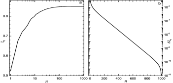
Figure 6: The convergence of $\xi_{1}$ in Eq. (15). This is the case for the minimal periodic orbit of rotation number $9/4$. (a) $\xi_{1}$ versus recursive number $n$; (b) The error versus $n$, where the error is defined as the difference $\Delta\xi_{1}=\xi_{1}(n)-\xi_{1}(1000)$.

We calculate $\xi_{1}(n)$ using a recursive algorithm. An example for the minimal periodic orbit of rotation number $9/4$ is shown in Fig. 6. The convergence of $\xi_{1}$ with the increasing recursive number $n$ can be seen clearly.

In a similar way, reversing the direction of calculation, we obtain $\xi_{-1}$, which is the projection of unstable direction on $x-$axis at point $(x_{-1},y_{-1})$. Considering

$$y_{0}=-S_{2}(x_{-1},x_{0}),$$

we compute the $y-$axis projection of the unstable direction at point $(x_{0},y_{0})$ through:

$$\eta^{\prime}_{0}=-S_{12}(x_{-1},x_{0})\xi_{-1}-S_{22}(x_{-1},x_{0})\xi_{0}$$ (17)

with $\xi_{0}=1$. And the unstable direction at point $(x_{0},y_{0})$ is $\vec{\rm r}_{u}=(1,\eta^{\prime}_{0})$.

Finally, the angle between the stable and unstable directions, i.e. the characteristic angle of the hyperbolic structure, can be calculated easily

$$\alpha=\arccos\left(\frac{\vec{\rm r}_{s}\cdot\vec{\rm r}_{u}}{|\vec{\rm r}_{s}|\,|\vec{\rm r}_{u}|}\right).$$ (18)

As examples of the above algorithm, we calculated the positions of a series of hyperbolic periodic orbits and their characteristic angles. Generally, the more irrational a rotation number is, the more robust the corresponding KAM torus is, and the stronger the stickiness effect is around the relics of the KAM torus after its breaking. People often write the rotation number in the form of continued fraction, on account of the merit of its direct relation to the “irrationality”. A continued fraction

$$a_{0}+\frac{1}{a_{1}+\frac{1}{a_{2}+\frac{1}{a_{3}+\cdots}}}$$

can be denoted by $[a_{0};a_{1},a_{2},a_{3},\cdots]$, where $a_{0}$ is the integer part of the number and $a_{i}$ are the positive integers. Any rational number can be expressed as a truncated continued fraction $[a_{0};a_{1},a_{2},a_{3},\cdots,a_{n}]$. And the integer $n$ will be called the “order” of the continued fraction in this paper. Note an $n$ th order continued fraction ended with $a_{n}=2$ is the same as an $(n+1)$ th order one ended with $a_{n}=1,a_{n+1}=1$.

Table 1: Angles between the stable and unstable manifolds of hyperbolic periodic orbits. The first 3 columns are the rotation numbers given in different forms, the forth column is the order of the continued fraction, and the last column is the angle (in degrees).

Rotation Number	Fraction	Continued Fraction	Order	Angle
2.5	5/2	[2;2]	1	169.573
2.6666$\cdots$	8/3	[2;1,2]	2	116.235
2.6	13/5	[2;1,1,2]	3	9.034
2.625	21/8	[2;1,1,1,2]	4	2.094
2.6153$\cdots$	34/13	[2;1,1,1,1,2]	5	1.042
2.6190$\cdots$	55/21	[2;1,1,1,1,1,2]	6	1.657
2.6176$\cdots$	89/34	[2;1,1,1,1,1,1,2]	7	0.742
2.6186$\cdots$	144/55	[2;1,1,1,1,1,1,1,2]	8	0.583

Several hyperbolic periodic orbits are calculated and the results are listed in Table 1. An obvious tendency derived from Table 1 is that, the bigger period number (the integer $p$ of the rotation number $q/p$) leads to the smaller characteristic angle. As the rotation number is getting more and more irrational the angle becomes smaller and smaller. It is well-known nowadays that the last KAM tori are those with the “noble” rotation numbers [34], i.e. the continued fractions that have $a_{k}=1$ for all $k$ above a certain number $N$. And the torus with the “golden rate” rotation number $(\sqrt{5}-1)/2=\left[0;1,1,1,\cdots,1,\cdots\right]$ is surely the most robust one. In our model, we see in Table 1 that the angle becomes smaller when the rotation number approaches this noble value. And also, we notice that the “difficult-to-cross partial barrier” and the most sticky region we mentioned in § 2.2 are just the region corresponding to this noble rotation number.

4 Stickiness effect and characteristic angle of hyperbolic structure

When the trajectory of an orbit is plotted on the phase space, we can see the trajectory points accumulate in some specific areas, indicating the existence of some structures causing stickiness effect. In this way we may obtain a direct impression of the sticky region, just as we have shown in Fig. 3. Considering a bunch of numerous orbits in the phase space, they may leave a certain region as time passes by. The survival probability of orbits in the definite region decays with time slowly. The slow decay is also an indicator of the stickiness effect [16, 17, 25]. Following these techniques, in this section we will show the diffusion routes of some typical orbits and find out where they are “stuck”. We will check the structures causing the stickiness effect in detail, and figure out the relation between the diffusion speed (or inversely, the stickiness effect) and the characteristic angle of hyperbolic structures in the sticky region.

4.1 Typical diffusion route

Due to the chaotic character, a chaotic orbit in its diffusion route may diffuse toward any direction at a moment. Since the upper part of the phase space is not open to a chaotic orbit but barred by KAM tori as we have seen in Fig. 1, an orbit will diffuse downward overall. To monitor the diffusion, we check the minimal $y$ value that an orbit attains on its trajectory in the phase space. During the diffusion, each time when the $y$ value reaches a new minimum $y_{\rm min}$, we record the time $t$. In such $(t,y_{\rm min})$ records, the “back and forth” motion in the diffusion is abandoned, and the “one-way” diffusion is emphasized.

Arbitrarily, two initial points $(x_{0},y_{0})=(0.49,29.0)$ and $(0.50,30.00001)$ are selected and their diffusions are followed. The temporal evolutions of the minimums of the $y$ value are shown in Fig. 7. Note only part of the orbits, when the minimums are smaller than $y=20.5$, is displayed. Each point $(t,y_{\rm min})$ in Fig. 7 tells that at time $t$ the orbit attains a new minimal value $y_{\rm min}$.

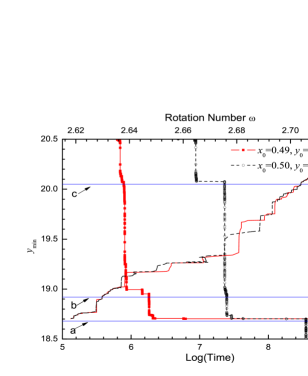
Figure 7: The variation of minimal $y$ of an orbit with respect to time (curves from upper left to lower right). The red solid squares are for the orbit initialized at $(0.49,29.0)$ and the black open circles for $(0.50,30.00001)$. The rotation numbers (indicated on the top $x$-axis) of orbits around the corresponding local lowest position are plotted (two curves crossing the panel from the lower left to upper right). Three regions that will be analyzed below are indicated by horizontal lines at $y_{\rm min}=20.05,18.92$ and $18.68$ (see text for explanations).

On the $(t,y_{\rm min})$ curve in Fig. 7, an orbit makes some steep “steps” and flat “plateaus”. A steep step indicates that the orbit diffuses very quickly in this stage, probably crossing a well-developed chaotic region or jumping over a wide island-chain. While a plateau indicates that the orbit spends a long time achieving a small advance in $y$ direction, i.e., it is facing an obstacle on its diffusion route. And the wider the plateau is, the more effective the obstacle is (the stronger stickiness effect it has).

Owning to the chaotic character, two orbits follow different diffusion routes and may suffer different stickiness effects, that’s why in Fig. 7 two curves differ from each other. But in the same phase space, the sticky regions that they have to pass through are the same, thus the plateaus appear at the same $y_{\rm min}$ on two curves. Note the logarithmic scale of the abscissa affects the apparent widths of the plateaus.

When an orbit reaches a new minimum $y_{\rm min}$ at moment $t$ during its diffusion, a temporary (local) rotation number $\omega$ of the orbit around this point is calculated. For each $y_{\rm min}$, we use 1001 orbital points (including the one right at moment $t$, 500 before and 500 after $t$) to estimate $\omega$. These records $(\omega,y_{\rm min})$ are plotted in Fig. 7 too, as the curves crossing the panel from lower left to upper right. On these curves, we can find the temporary rotation number ($\omega$, indicated on the top $x$ axis) for each $y_{\rm min}$. Again, the jumping of $\omega$ implies that the orbit is temporarily in the vicinity of a big island, while the (nearly) continuous variation of $\omega$ implies that the orbit is crossing a series of finely ground island-chains, or a cantorus. The consistence between the continuous variation of $\omega$ and the wide plateau of $y_{\rm min}$ is evident in Fig. 7.

Combining the explorations on the diffusion routes in § 2.2 and in Fig. 7, we know that an orbit meets considerable resistance when crosses some regions, where the $(t,y_{\rm min})$ curves make plateaus and the $(\omega,y_{\rm min})$ curves vary continuously. We choose three such “sticky regions” to investigate in detail in the following part of this paper. Three horizontal lines in Fig. 7 show the lower bounds of these regions. Particularly, the lowest one is close to wide plateaus on the $(t,y_{\rm min})$ curves, indicating a strong stickiness effect around it. Checking the rotation number, we see that it is close to the golden rate. To explain clearly the “sticky region”, here we define the sticky region labeled Region c as an example. A lower bound $y_{c}^{l}=18.68$, as shown in Fig. 7, is set first. For an orbit starting from an initial point above this lower bound, if the $y$ value of this orbit gets smaller than $y_{c}^{l}$ for the first time during its diffusion, we regard the orbit as having crossed Region c. An upper bound $y_{c}^{u}$ is selected as well. When the $y$ value of an orbit gets smaller than $y_{c}^{u}$ for the first time, the orbit is defined as having entered Region c. The difference between the upper and lower bound $\delta y_{c}=y_{c}^{u}-y_{c}^{l}$ is the width of this sticky region.

It is worth to note that there is no clear/sharp boundary for a sticky region in the above definition. Although we use a $y_{\rm min}$ value to denote it, we should keep in mind that a sticky region is not a straight (but most probably curved) belt across the phase space.

4.2 Characteristic angle of hyperbolic structure and diffusion speed

To explore the stickiness effects in these sticky regions, first we plot in Fig. 8 part of the phase space in detail around the corresponding local minimum $y_{\rm min}$ where orbits feel the considerable resistance along their diffusion routes.

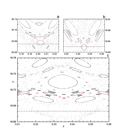
Figure 8: Three sticky regions. Three panels are for the regions indicated by arrows in Fig. 7 (see text). Horizontal lines in each panel represent the line of $y=20.05,y=18.92$ and $y=18.68$, respectively. The island chains in red are the ones with the highest period number found in the region.

According to Birkhoff theorem [see e.g. 31], the elliptic periodic orbits and hyperbolic periodic orbits emerge in pairs after the breaking of the invariant tori in a 2D mapping. The elliptic periodic orbits locate in the centers of islands, while the hyperbolic periodic orbits exist between every two adjacent islands in an island-chain. These two types of periodic orbits share the same rotation number. The diffusion of an orbit is through these hyperbolic structures.

The elliptic periodic orbits are surrounded by invariant curves and they together make islands. The hyperbolic periodic orbits however are unstable and the geometric structures around them are not as visible as the islands. So we plot in Fig. 8 as many as possible the island chains to imply the positions of hyperbolic periodic orbits and to show the composition of the sticky regions. In each region, the island chain with the highest periods (they are 71, 73 and 144 in Region a, b and c) have been plotted in red. Of course, there must be islands of even higher periods, but their sizes are much smaller, and it is impossible to plot all of them in practice. The hyperbolic periodic points can be located and the characteristic angles of the hyperbolic structures can be calculated, using the algorithm introduced in above section. Some characteristic angles in these regions are summarized in Table 2.

Table 2: Characteristic angles of hyperbolic structures in three sticky regions. The hyperbolic periodic orbits are denoted by their rotation numbers, given in normal fraction numbers and continued fractions. The angles are in degrees.

Region a
Rotation number
Fraction	Continued Fraction	Angle $(\alpha)$
165/61	[2;1,2,2,1,1,3]	0.718653
119/44	[2;1,2,2,1,1,2]	0.845155
192/71	[2;1,2,2,1,1,1,2]	0.772372
73/27	[2;1,2,2,1,2]	1.094884
Region b
171/65	[2;1,1,1,2,2,3]	0.717274
121/46	[2;1,1,1,2,2,2]	0.863938
192/73	[2;1,1,1,2,2,1,2]	0.777229
71/27	[2;1,1,1,2,3]	1.179671
Region c
199/76	[2;1,1,1,1,1,1,1,3]	0.506420
343/131	[2;1,1,1,1,1,1,1,2,2]	0.472460
144/55	[2;1,1,1,1,1,1,1,2]	0.582802
377/144	[2;1,1,1,1,1,1,1,1,1,2]	0.477654
233/89	[2;1,1,1,1,1,1,1,1,2]	0.534822
89/34	[2;1,1,1,1,1,1,2]	0.741975

We have seen from Table 1 that the characteristic angles of hyperbolic structures with higher period numbers are smaller. This trend can be seen again in each region in Table 2. But when considering the characteristic angles with nearly the same period number in different regions, for example, the characteristic angles corresponding to the rotation number 192/71 in Region a, 192/73 in b and 199/76 in c, we find that the angle in Region c $(0.506^{\circ})$ is significantly smaller than the other two in Regions a $(0.772^{\circ})$ and b $(0.777^{\circ})$, while the latter two are nearly equal to each other. This result is expectable since Region c makes the widest plateau in Fig. 7 and the diffusion time through this region is in the order of $10^{8}\sim 10^{9}$, much longer than that in Regions a and b.

The characteristic angle may decreases as the period of orbits increases, but it is impossible in practice to compute the characteristic angles for all the hyperbolic structures. Fortunately, the information about the smallest characteristic angle in a region can still be obtained. In Region c, the rotation numbers of the hyperbolic periodic orbits is close to the “golden rate”, and it is well-known that the KAM torus with the golden rate rotation number is the most robust one. Meanwhile, it is natural to assume that the “smallest” characteristic angle should be found in the hyperbolic structures of the new-born cantorus just after the breaking of KAM torus. Since the golden rate can be approached by continued fractions, the characteristic angles of hyperbolic structures with rotation numbers of truncated continued fractions may approach to the characteristic angle in the cantorus. Following this idea, we continue the calculations listed in Table 1 to higher order of the continued fraction. The variation of the characteristic angle with respect to the order of the continued fraction is illustrated in Fig. 9. Note, as the order increases the corresponding periodic orbits tend to gather around the golden rate cantori, and no later than the 7th order (89/34) all the hyperbolic structures under consideration accumulate in Region c.

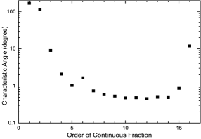
Figure 9: The lower bound of characteristic angles in Region c. The abscissa is the order of the truncated continued fraction, which is the rotation number of the hyperbolic periodic orbit. The ordinate is the corresponding characteristic angle. The last point of order 16 represents the hyperbolic periodic orbit with rotation number 10946/4181.

As shown in Fig. 9, the calculations are stopped at the 16th order where the rotation number is 10946/4181. We cease the calculations for two reasons as follows. First, the calculations so far have shown that the characteristic angle has a lower bound when the truncated continued fractions approach the golden rate. Even higher order does not decrease this lower bound. Second, calculations for the high order continued fractions (therefore high period number) are very expensive in computer time, and it is difficult to control the error in this case because we have to deal with a large number of linear equations (Eq. (15)). So we adopt the smallest angle in Fig. 9 at the 12th order, $\alpha_{c}=0.457^{\circ}$, as the lower bound of the characteristic angle in Region c.

For Regions a and b, there is no golden rate rotation number. However we can follow a similar process as we have done for Region c to calculate the lower bound of characteristic angles. We expand the continued fractions listed in Table 2 by inserting number ‘1’ into them right before the last number, then we have series of truncated continued fractions of different orders. Adopting these continued fractions as the rotation numbers, we calculate the characteristic angles of the corresponding hyperbolic structures. In this way, we obtain the lower bound of the characteristic angles $\alpha_{a}=0.665^{\circ}$ in Region a and $\alpha_{b}=0.667^{\circ}$ in Region b.

Since $\alpha_{a}\approx\alpha_{b}>\alpha_{c}$, we may derive directly from these values that the diffusion in Region c is slower than that in Regions a and b. In other words, the stickiness effect in Region c is more intensive than that in Regions a and b, while Regions a and b have nearly the same stickiness effects. To verify this conclusion, we carry out some calculations of diffusion speed below.

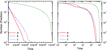
Figure 10: The diffusion speeds of orbits in Regions a, b and c. The time is given in linear scale in left panel, and logarithmic scale in right panel.

The diffusion speed, generally is measured by the decay rate of the survival numbers of a bunch of orbits in a defined area [8, 16, 17]. We set randomly $40,000$ initial points in a rectangle from $(0.45,26.5)$ to $(0.55,31.5)$ around the hyperbolic fixed point of rotation number $3/1$ that is embedded in a developed chaotic area and above the Regions a, b and c in the phase space (see Fig. 1). All the orbits are iterated for $10^{9}$ times using the mapping. The evolution of these forty thousand orbits are then followed, especially, we monitor the variation of the action variable $y$ of each orbit.

The definition of sticky region has been introduced in § 4.1. For Regions a, b and c, the lower boundaries are chosen to be $y_{a}^{l}=20.05,y_{b}^{l}=18.92,y_{c}^{l}=18.68$ respectively, as indicated by the horizontal lines in Figs. 7 and 8. After some tests, we set the width of the sticky region $\delta y=0.1$ for all three regions. The upper boundaries of the sticky regions are then defined as $y_{a,b,c}^{u}=y_{a,b,c}^{l}+\delta y$.

An orbit may wander for quite a while before it enters a specific area. To exclude the evolution history before an orbit entering the vicinity of Region a, b or c, we define the moment $t_{a}^{u}$ (or $t_{b}^{u},t_{c}^{u}$) when for the first time the $y$ value of an orbit is smaller than the upper boundary $y_{a}^{u}$ (or $y_{b}^{u},y_{c}^{u}$) as the moment of entering Region a (or Region b, c). On the other hand, when an orbit satisfies for the first time $y<y_{a}^{l}$ (or $y_{b}^{l},y_{c}^{l}$) at moment $t_{a}^{l}$ (or $t_{b}^{l},t_{c}^{l}$), it is regarded as having escaped from the sticky region. The time duration $\Delta t_{a,b,c}=t_{a,b,c}^{l}-t_{a,b,c}^{u}$ then is defined as the surviving time of an orbit in the corresponding sticky region. Following the evolution of the 40,000 orbits, we record the surviving time of each orbit in three sticky regions. With these records, we count how many orbits survive in a specific region at a given surviving time. Some orbits may have been initialized on invariant curves by chance, and a small number of orbits may wander in the chaotic phase space but never reach a specific region. These orbits are excluded from the final statistics. After removing these orbits and normalizing the number of orbits at the beginning to unit, the diffusions in the three regions are summarized in Fig. 10.

Apparently, the diffusion is quick in Regions a and b, but slow in Region c, reflecting that the stickiness effect in Region c is much stronger than in other regions. On the other hand, although Regions a and b occupy different areas in the phase space and they comprise different components as shown in Fig. 8, they have nearly the same diffusion speed. The results are consistent with the conclusion we derived from the characteristic angle values.

4.3 Characteristic angle and perturbation parameter

So far we have seen that in the phase space of a mapping with given perturbation parameter $k$, the stickiness effects of different sticky regions are related to the characteristic angles of hyperbolic structures embedded in the regions. Smaller characteristic angles lead to stronger stickiness effects and slower diffusions. Below we will investigate the relation between the stickiness effect and the characteristic angle when the parameter $k$ changes. We will focus on the Region c where the diffusing orbits suffer the most significant stickiness effects as shown above.

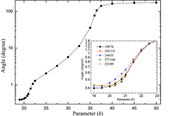
Figure 11: The variation of characteristic angle with respect to the parameter $k$. The solid circles show the angle of the hyperbolic structure with rotation number $199/76$. The embedded panel shows the characteristic angles of several hyperbolic structures with different rotation numbers.

In Region c, we select five hyperbolic periodic orbits to analyze, including the one with rotation number 377/144 for which the corresponding island-chain was plotted in red in Fig. 8, three above it with rotation numbers 199/76, 343/131 and 144/55, and one below it with the rotation number 233/89. The corresponding island chains are all plotted in Fig. 8, and they stay close to each other in a narrow area in the phase space. Their characteristic angles at different $k$ values are then calculated . The results are illustrated in Fig. 11 and some of them are listed in Table 3 too.

Table 3: The characteristic angles at different parameter $k$. The angles are in degrees. Only five hyperbolic structures in Region c are listed here.

	Angle $(\alpha)$
Rot. Num.	$k=19.00$	$20.35$	$21.50$	$22.50$	$27.50$	$32.50$	$36.00$
199/76	0.396155	0.448865	0.792791	1.291957	3.288836	11.42482	77.06509
343/131	0.429506	0.426083	0.799331	1.294550	3.288836	11.42482	77.06509
144/55	0.405655	0.504247	0.851525	1.295668	3.288836	11.42482	77.06509
377/144	0.431027	0.437425	0.840257	1.314751	3.288844	11.42482	77.06509
233/89	0.431263	0.467751	0.856823	1.314805	3.288844	11.42482	77.06509

When $k$ is small, the global KAM tori exist in Region c and these hyperbolic structures are bounded by these tori. As pointed out in several literatures [e.g. 27, 36], in the vicinity of an invariant torus in a 2D phase space, the resonances (island-chains and hyperbolic periodic orbits) accumulate geometrically toward the torus with their increasing orders (period numbers). Owning to continuity, the directions of the stable and unstable manifolds of the hyperbolic structures are “forced” to be nearly parallel to the torus, thus the characteristic angles are quite small in the close neighborhood of a torus. Here we see from the embedded panel in Fig. 11 that the angles seem to approach a limit slowly as $k$ decreases. Consequently, orbits starting from the close vicinity of an invariant torus will diffuse along the resonance line (high-order island-chain) for a long time before its leaving for adjoining resonances. As $k$ increases, the chaos is developed and the characteristic angle increases. Particularly, after the global KAM tori disappear in this region (when $k\gtrsim 20.75$) the characteristic angle increases dramatically. As a result, the diffusion speed is expected to be enhanced dramatically.

Another interesting phenomenon is the difference between the characteristic angles of different rotation numbers. When $k$ is small, the characteristic angles are small and the relative difference between different rotation numbers is considerable. But the relative difference becomes smaller as the angles increase and almost invisible when $\alpha\sim 2^{\circ}(k=25)$. This is clearly illustrated in the embedded picture in Fig. 11. The reason is that the difference of hyperbolicity between different periodic orbits is apparent when $k$ is small, but it becomes ignorable when $k$ is large. In the latter case, chaos has developed, making the whole region uniformly hyperbolic. Thanks to this observation, to show the angle variation in a wide $k$ range, it is enough to follow just one of the hyperbolic structures, e.g., the one shown in Fig. 11 with rotation number $199/76$.

4.4 Stickiness effect and characteristic angle

The stickiness effect (or the diffusion speed) changes when the characteristic angle changes with $k$. We will present the relation between the diffusion speed and the size of characteristic angle in this part. To show this correspondence, we need to define the diffusion speed at first. The time needed by a bunch of orbits to cross through a definite sticky region may be a good measure. But a “sticky region” may deform as the structure of phase space distorts with the varying parameter $k$. Thus we check first the variation of the position of a hyperbolic periodic orbit at different $k$.

We plot in Fig. 12 the hyperbolic periodic orbit of rotation number $377/144$ at six $k$ values. As $k$ increases, the profile of the hyperbolic periodic orbit is distorted. The other four hyperbolic periodic orbits of rotation numbers 199/76, 343/131, 144/55 and 233/89 are calculated too, and we find that their profiles are distorted in a similar way as shown in Fig. 12 and they always stay together within a narrow area in the phase space. Therefore, the “sticky region” for different $k$ can be defined in a similar way as in § 4.2.

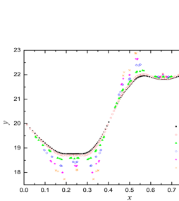
Figure 12: The positions of the hyperbolic periodic orbits of rotation number $377/144$. Cases of different $k$ are represented by different symbols.

Just as we have done for the case $k=20.75$, forty thousand points initialized in the rectangle area are followed again for different $k$ values. We now focus only on the Region c where the above mentioned five hyperbolic periodic orbits are embedded. Knowing the locations of these hyperbolic structures (as shown in Fig. 12), the “sticky region” at different $k$ is defined again. And also, the surviving time of an orbit in the sticky region is given by the time duration $\Delta t=t^{l}-t^{u}$ as before.

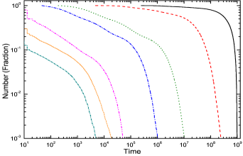
Figure 13: The diffusion at different $k$. From top to down (right to left), the curves represent the case for $k=20.75$, 21.00, 21.50, 22.50, 25.00, 27.00 and $k=30.00$, respectively.

All the orbits are iterated for $10^{9}$ times. We record the duration time $\Delta t$ of each orbit, and it is regarded as the surviving time of the orbit in the sticky region. The number of surviving orbits changes with time. Following the same technique for plotting Fig. 10b, we summarize our calculations for several $k$ in Fig. 13.

It is clear that the diffusion speeds up as $k$ increases. For the case of $k=20.75$, the first orbit escaping happens at $t\sim 2\times 10^{5}$, when more than 90 percent of orbits have escaped in the case of $k=22.50$. Nearly all orbits of $k=25.0$ and $k=27.00$ escape before $t\sim 10^{4}$, while only 1 percent of orbits survive after only hundreds of iterations for $k=30.00$.

In many literatures [e.g. 8, 16, 17, 35], the diffusion curves similar to the ones in Fig. 13 were fitted by a power law $N_{\rm survival}\propto t^{-z}$. The exponent $z$ then can serve as a measurement of the diffusion speed (or the intensity of the stickiness effect). But such a power law is not so distinct in our cases as we see in Fig. 13. Instead, we use directly the time when most of the orbits have escaped to measure the diffusion speed, (or inversely, the intensity of stickiness effect). More or less arbitrarily, we adopt the moment when 90 percent of orbits have escaped, denoted by $t_{1/10}$ since only one tenth of orbits survive at this moment, as an estimation of the diffusion speed. Thus a quick diffusion has a small $t_{1/10}$ while a large $t_{1/10}$ indicates a slow diffusion (and strong stickiness effect).

Figure 14: The variation of escaping time with respect to the characteristic angle ($\alpha$). The abscissa is $\cot\alpha=1/\tan{\alpha}$ and the ordinate is the escaping time ($t_{1/10}$, see text for definition) in logarithm. Several $\alpha$ values are indicated along the top axis too.

For $k$ varying from 20.75 to 30.00, we calculate the $t_{1/10}$ and the characteristic angles in this region at these $k$ values are computed as well. They are illustrated in Fig. 14. A small characteristic angle leads to a slow diffusion, that is, a large $t_{\rm 1/10}$. So, to visualize the variation of diffusion speed at small characteristic angle, we use $1/\tan{\alpha}$ instead of $\alpha$ itself as the abscissa in Fig. 14, while several $\alpha$ values are indicated along the top axis. The ordinate is the diffusion speed $t_{1/10}$ in logarithm scale. For a given parameter $k$, the characteristic angle in Fig. 14 is the lower bound of the characteristic angles in Region c. They are calculated in the same way that we have introduced in § 4.2.

As indicated by Fig. 14, the stickiness effect is significant only when the characteristic angle is small. When the characteristic angle $\alpha\sim 5^{\circ}(1/\tan\alpha=11.5)$, most of orbits have escaped just after tens of iterations, implying a weak stickiness effect. On the other end of smaller $\alpha$ in Fig. 14, the escaping time will be longer than $10^{9}$ when $\alpha$ is smaller than $0.45^{\circ}(1/\tan 0.45^{\circ}=127.3)$. An orbit with such a long diffusion time can be practically regarded as stable (never escape). In fact, the global KAM curves exist in Region c when $k\lesssim 20.5$. And the characteristic angle is smaller than $0.45^{\circ}$ when $k<20.5$, as we can see from Fig. 11.

It is worth to note that the points in Fig. 14 may be fitted by two linear functions with a crossover around $\alpha\sim 1^{\circ}$. The possible mechanism underneath such a relation deserves an investigation in future.

When $k\gtrsim 20.75$, all the global KAM tori in Region c have broken. The stickiness effect suffered by an orbit crossing this region arises from the island-chains and cantori embedded in the region. The diffusion speed is then determined by the characteristic angle of hyperbolic structures among the island-chains and cantori. Generally, in the vicinity of invariant tori, hyperbolic structures accumulate, thus the stickiness effect felt by orbits close to the tori, where the stickiness effect was firstly found and defined [kar82, kar83], has the same origin: the hyperbolic structures.

5 Conclusions

The stickiness effect in the phase space is an interesting phenomenon with implications in many areas of sciences. It has attracted many attention in the fields of mathematics, physics and astronomy. Many structures such as the KAM tori, the island chains, the cantori, and the hyperbolic structures in the phase space are found to have stickiness effect. Among them, we think the hyperbolic structures play the essential role, as we have shown in our previous papers.

In this paper, we describe some geometric details of the hyperbolic structure, especially the angle between the stable and unstable manifolds, and relate these geometric characters with the strength of the stickiness effect.

Usually the recursive algorithm is employed to calculate the positions of periodic orbits in the phase space. But a usual recursive algorithm fails when we try to find the hyperbolic periodic orbits, because the set of hyperbolic periodic orbits is of measure zero when the system is far from the integrable one. In this paper, a numerical algorithm is introduced, with which we can compute the precise locations of the hyperbolic periodic orbits. And also, a practical algorithm for computing the directions of stable and unstable manifolds of the hyperbolic structures is presented.

With these numerical algorithms, we have computed the angles between the stable and unstable manifolds in different hyperbolic structures in the 2D phase space of a mapping model. We investigate the stickiness effect (diffusion speed) in different regions of the phase space, and how it changes with the perturbation parameter.

Our findings in these calculations may be summarized as below:

- In an area where the last KAM torus has broken, the characteristic angle between the stable and unstable manifolds of the hyperbolic structure is related to the rotation number. The more irrational the rotation number is, the smaller the angle is. But a lower bound of this angle exists in a certain region.

- The stickiness effect (diffusion speed) is determined by the characteristic angle. The smaller the angle is, the slower the diffusion is, alternatively speaking, the stronger the stickiness effect it has.

- A relationship between the characteristic angle of the hyperbolic structure and the stickiness effect has been revealed. Nevertheless, it is still difficult to find a quantitative way to describe this relationship explicitly.

Although the above conclusions are drawn from the calculations in regions consisted of island-chains and cantori but not global invariant tori, they should be valid for all structures proven to possess stickiness effect.

This work was supported by the Natural Science Foundation of China (NSFC, No. 10833001, No. 11073012) and by Qing Lan Project (Jiangsu Province). Li and Sun are also supported by the National Basic Research Program of China (2013CB834103) and by NSFC (No. 11078001, No. 11003008).

1 Karney C F, Rechester A B, White R B. Effect of noise on the standard mapping. Physica D, 1982, 4: 425–438

2 Karney C F. Long-time correlations in the stochastic regime. Physica D, 1983, 8: 360–380

3 Zaslavsky G M, Edelman M, Niyazov B A. Self-similarity, renormalization, and phase space nonuniformity of Hamiltonian chaotic dynamics. Chaos, 1997, 7: 159–181

4 Zaslavsky G M. Chaos, fractional kinetics, and anomalous transport. Phys Rep, 2002, 371: 461–580

5 Barash O, Dana I. Type specification of stability islands and chaotic stickiness. Phys Rev E, 2005, 71: 036222

6 Abdullaev S S. Chaotic transport in Hamiltonian systems perturbed by a weak turbulent wave field. Phys Rev E, 2011, 84: 026204

7 Custódio M S, Beims M W. Intrinsic stickiness and chaos in open integrable billiards: Tiny border effects. Phys Rev E, 2011, 83: 056201

8 Jaffé C, Ross S D, Lo M W, et al. Statistical Theory of Asteroid Escape Rates. Phys Rev Lett, 2002, 89: 011101

9 Karne C F, Bers A. Stochastic ion heating by a perpendicularly propagating electrostatic wave. Phys Rev Lett, 1977, 39: 550–554

10 Beloshapkin V V, Chernikov A A, Natenzon M Ia, et al. Chaotic streamlines in pre-turbulent states. Nature 1989, 337: 133–137

11 Chia P-K, Schmitz L, Conn R W. Stochastic ion behaviour in subharmonic and superharmonic electrostatic waves. Phys Plasmas, 1996, 3: 1545–1568

12 Fromhold T M, Patane A, Bujkiewicz S, et al. Chaotic electron diffusion through stochastic webs enhances current flow in super lattices. Nature, 2004, 428: 726–730

13 Varga I, Pollner P, Eckhardt B. Quantum Localization near Bifurcations in Classically Chaotic Systems. Annalen der Physik, 1999, 8: 265-268

14 Kalapotharakos C, Voglis N, Contopoulos G. Chaos and secular evolution of triaxial N-body galactic models due to an imposed central mass. Astron Astrophys, 2004, 428: 905–923

15 Chirikov B, Shepelyansky D L. Correlation properties of dynamical chaos in Hamiltonian systems. Physica D, 1984, 13: 395–400

16 Meiss J D, Ott E. Markov-tree model of intrinsic transport in Hamiltonian systems. Phys Rev Lett, 1985, 55: 2741–2744

17 Lai Y C, Ding M C, Grebogi C, et al. Algebraic decay and fluctuations of the decay exponent in Hamiltonian systems. Phys Rev A, 1992, 46: 4661–4669

18 Perry A D, Wiggins S. KAM tori are very sticky: rigorous lower bounds on the time to move away from an invariant Lagrangian torus with linear flow. Physica D, 1994, 71: 102–121

19 Contopoulos G, Voglis N, Efthymiopoulos C, et al. Transition spectra of dynamical systems. Celest Mech Dyn Astron, 1997, 67: 293–317

20 Froeschlé Cl, Lega E. Modeling mappings: an aim and a tool for the study of dynamical systems. In: Analysis and Modeling of Discrete Dynamical Systems. Benest D, Froeschlé Cl. eds. 1998, 3-54

21 Sun Y S, Fu Y N. Diffusion character in four-dimensional volume preserving map. Celest Mech Dyn Astron, 1999, 73: 249–258

22 Contopoulos G, Harsoula M, Voglis N, et al. Destruction of islands of stability. J Phys A: Math Gen, 1999, 32: 5213–5232

23 Contopoulos M, Harsoula M. Stickiness effects in chaos. Celest Mech Dyn Astron, 2010, 107: 77–92

24 Efthymiopoulos C, Contopoulos G, Voglis N. Cantori, islands and asymptotic curves in the stickiness region. Celest Mech Dyn Astron, 1999, 73: 221–230

25 Sun Y S, Zhou L Y, Zhou J L. The role of hyperbolic invariant sets in stickiness effects. Celest Mech Dyn Astron, 2005, 92: 257–272

26 Sun Y S, Zhou L Y. Stickiness in three-dimensional volume preserving mappings. Celest Mech Dyn Astron, 2009, 103: 119–131

27 Morbidelli A, GiorgilliA. Superexponential stability of KAM tori. J Stat Phys, 1995, 78: 1607–1617

28 Howard J E, Humpherys J. Nonmonotonic twist maps. Physica D, 1995, 80: 256–276

29 Chirikov R V. A universal instability of many-dimensional oscillator systems. Phys Rep, 1979, 52: 263–379

30 Cheng J, Sun Y S. Stable and Unstable Properties of the Standard-liked Map. Random & Computational Dynamics, 1996, 4: 73–85

31 Siegel C L, Moser J K. Lectures on Celestial Mechanics, 1971, Springer-Verlag, Berlin

32 Bangert V. Mather sets for twist maps and geodesics on tori. Dynamics Reported, 1988, 1: 1 C56

33 Cheng J. Variational approach to homoclinic orbits in twist maps and an application to billiard systems. Z angew Math Phys, 2004, 55: 400–419

34 Greene J M. A method for determining a stochastic transition. J Math Phys, 1979, 20: 1183–1201

35 Benegeroles R. Universality of Algebraic Laws in Hamiltonian Systems. Phys Rev Lett, 2009, 102: 064101

36 Zhou J L, Zhou L Y, Sun Y S. Hyperbolic Structures and the Stickiness Effect. Chin Phys Lett, 2002, 19: 1254–1256