Coupling of matter and radiation at supernova shock breakout

Abstract

Some features of the physics of radiation-dominated shock waves are discussed with emphasis on the peculiarities which are important for correct numerical modeling of shock breakouts in supernova. With account of those peculiarities, a number of models for different supernova types is constructed based on multigroup radiation transfer coupled to hydrodynamics. We describe the implementation of a new algorithm rada, designed for modeling photon transfer at extremely-relativistic motions of matter, into our older code stella. The results of numerical simulations of light curves, and continuum spectra are presented. The influence of effects of photon scattering on electrons, of thermalization depth and of special relativity in transfer equation is considered. Some cases are demonstrated, when the appearance of hard X-ray emission is possible at the shock breakout. The necessary refinements in numerical algorithms for radiative transfer and hydrodynamics are pointed out. Prospects for using the results of numerical simulation to analyze and interpret available and future data from space observatories are discussed.

1 Introduction

The phenomenon of a supernova in most cases should start with a bright flash, caused by a shock wave emerging on the surface of the star after the phase of collapse or thermonuclear explosion in interiors. The detection of such outbursts associated with the supernova shock breakout can be used to obtain information about the explosion properties and presupernova parameters, which is necessary to understand the physical processes that underlie this phenomenon.

For an accurate treatment of the shock wave propagation near the surface of a presupernova it is necessary to perform numerical calculations which, in addition to hydrodynamics, should account correctly for radiative transfer in moving media. In some cases, e.g. in compact type Ib/c presupernovae, shock waves can reach relativistic velocities (Blinnikov et al., 2002; Blinnikov et al., 2003). Then one has to include into consideration a number of relativistic effects. This paper presents the results of numerical simulation of shock waves in several models for type Ib and type II supernovae, taking into account these features.

Studying the supernova shock breakout becomes particularly topical in connection with the recent detection of this phenomenon by the SWIFT spacecraft (Soderberg et al., 2008). In addition, a flash from the shock wave on the surface of red supergiant in type II supernova SNLS-04D2dc (Schawinski et al., 2008; Gezari et al., 2008) and light echo from the shock wave of Cas A (Dwek & Arendt, 2008) are detected. Simulations (Tominaga et al., 2009, 2011) with our code stella show good agreement with observations in case of SNLS-04D2dc. The enormous luminosity of SN 2006gy is most successfully explained by models where the radiative shock wave provides almost all radiation for many months (Woosley, Blinnikov & Heger, 2007). There is a possibility of obtaining new data if the experiments similar to LOBSTER space observatory (Calzavara & Matzner, 2004), the satellite EXIST (Energetic X-ray Imaging Survey Telescope, see Grindlay et al., 2003; Band et al., 2008) or any X-ray station of a similar type would be launched in the future. E.g., the experiment MAXI (Monitor of All-sky X-ray Image) on board the module Kibo at ISS (Matsuoka et al., 1997) is already started.

In this paper we compare the results of the predictions for shock breakout for three codes: the equilibrium diffusion gray radiation-hydro code snv, nonequilibrium multigroup radiation-hydro code stella and ultrarelativistic nonequilibrium multigroup transfer code rada. We check the sensitivity of the predictions of the shock emission to the parameters of the numerical scheme, such as the boundaries of the frequency interval (including the X-ray range), and to the approximations in the opacity description. It is found that high-temperature peak behind the shock front and production of hard “tail” in spectrum are suppressed by extremely low true absorption, with a cross-section at the level $10^{-6}$ of Thomson scattering in a presupernova SN Ib. This level of absorption can be provided by double Compton effect (Mandl & Skyrme, 1952; Weaver, 1976; Lightman, 1981), so it must be taken into account in realistic models of radiation-dominated shock waves in a supernova. Some additional refinements necessary in the methods of constructing shock-breakout models are pointed out. Among them we consider how the relativistic and geometric effects in radiative transfer in a comoving frame of reference influence the predictions of supernova light curves and spectra at the epoch of shock-breakout.

2 Radiation dominated shock waves

Let us consider some of the peculiarities of a shock wave when one cannot neglect radiation, and, moreover, when the shock front structure is determined by energy and momentum of photons. This situation is typical for supernova explosions, therefore, its description is important for building adequate models.

There are many theoretical articles and several books where properties of radiation-dominated shock are considered. In most theoretical works it is supposed that the medium is optically thick, i.e. photons born in the shock waves are absorbed by the cold matter upstream. This pictures holds in a stellar explosion before the actual outburst of supernova light while the shock is still buried under the photosphere.

A brief review of the contributions that are important for the history of the problem is given by Blinnikov & Tolstov (2011). Below we mention only the papers most important for further discussion.

A very detailed study of shock structure with radiation has been performed by Weaver (1976): he has shown that production of observable hard (gamma-ray) radiation at supernova shock breakout is very problematic. Nevertheless, Blandford & Payne (1981b, a) have predicted the possibility of a nonthermal “tail” in spectra born in shock waves in hot media. However, these authors have neglected a number of effects associated with Compton scattering taken into account by Weaver (1976). Further refinement of the theory with regard to the thermal Compton effect has been made by Lyubarskii & Syunyaev (1982), Fukue, Kato & Matsumoto (1985), Becker (1988) and other researchers.

Discontinuities inevitably develop in gas parameters in a shock wave which is not too weak and not too strong (while radiation energy and momentum can be neglected), if one takes into account only thermal conduction and neglects viscosity (see section VII.3 in Zeldovich & Raizer, 1966). In real gases the discontinuities are smoothed by viscosity which transforms the ordered motion (kinetic energy of the flow) into the heat (chaotic motion of particles) on the distance of the order of one mean free path of particles. This is called a viscous jump (Zeldovich & Raizer, 1966; Shu, 1992). At very high amplitudes of the shock, when the energy density and pressure of radiation become large in comparison with those of matter, the situation is different and the viscous jump disappears. Gas goes from the initial state to the final one under the action of radiative heat conduction, even if the viscosity of matter is not taken into account (Belokon, 1959). Such a situation is achieved when radiation pressure $P_{r}$ and the gas pressure $P_{g}$ behind the shock front are related as $P_{r}/P_{g}\simeq 4.4$.

Imshennik & Morozov (1964) analysed various options for transfer equation (simple diffusion equation and the Eddington approximation in the moving medium). Plasma upstream the shock front was taken to be cold ($T_{0}=0,\;P_{g}=0$). Their solution is more rigorous than presented by (Belokon, 1959) and it yields $P_{r}/P_{g}\simeq 8.5$ for the condition of disappearance of viscous jump. The compression in the shock should then exceed a critical value $\rho_{1}/\rho_{0}=6.68$. However, see Weaver & Chapline (1974), where it is again obtained $P_{r}/P_{g}\simeq 4.4$. It should be noted that in determining the structure of the shock front, the flux of photon momentum, i.e. the radiation pressure, begins to play a role comparable to the flux of energy. Such conditions are often achieved in astrophysical shock waves, in particular, in supernovae.

The viscous density jump disappears during propagation of the shock wave inside of a presupernova if radiation pressure is appreciably higher than the plasma pressure and when there is a fairly intense processes of absorption and creation of photons, not just their pure monochromatic scattering. Note that Imshennik & Morozov (1964) assumed extinction equal to the true absorption, scattering was not taken into account.

Calculations of Weaver (1976) have been performed in the diffusion approximation with a simplified description of Compton scattering and various processes of absorption and creation of photons, and they have resulted in a critical ratio $P_{r}/P_{g}\simeq 4.45$. He assumed that the radiation has an equilibrium blackbody spectrum. This was criticized by Blandford & Payne (1981b, a); Riffert (1988); Becker (1988). In our work, we make no assumptions about the equilibrium of radiation, and take into account in the calculations of the evolution of photons the same terms as Blandford & Payne (1981b, a). Nevertheless, our results are closer to the results of Weaver (1976), than to the results of his critics: we show that the achievement of high temperatures in the radiation-dominated shock waves is unlikely with a realistic allowance for the photon production processes.

An important parameter is the optical depth $\tau_{k}$ of the heating zone for strong shocks. In the approximation of Imshennik & Morozov (1964),

$$\tau_{k}\sim{12c\over 7D_{s}}\;,$$ (1)

where $D_{s}$ is the shock front velocity and $c$ is the speed of light. The approximate solution by Klimishin (1968) uses the concept of a critical temperature $T_{k}$, introduced by Raizer (1957). The solution by Klimishin (1968) is closer to the conditions of supernovae than the solution by Imshennik & Morozov (1964), because $T_{k}$ in supernovae is low at a low density. It gives

$$\tau_{k}\sim{14c\over 3D_{s}},$$ (2)

i.e., a value of the same order of magnitude.

Thus, the shock wave propagates without energy losses as long as the lower limit on the optical depth holds (Ohyama, 1963; Imshennik & Morozov, 1964; Chevalier, 1981; Imshennik & Nadezhin, 1989):

$$\tau=\frac{\delta R}{l}\mathrel{\mathchoice{\lower 3.6pt\vbox{\halign{$\mathsurround=0pt\displaystyle\hfil#\hfil$\cr>\crcr\sim\crcr}}}{\lower 3.6pt\vbox{\halign{$\mathsurround=0pt\textstyle\hfil#\hfil$\cr>\crcr\sim\crcr}}}{\lower 3.6pt\vbox{\halign{$\mathsurround=0pt\scriptstyle\hfil#\hfil$\cr>\crcr\sim\crcr}}}{\lower 3.6pt\vbox{\halign{$\mathsurround=0pt\scriptscriptstyle\hfil#\hfil$\cr>\crcr\sim\crcr}}}}\frac{c}{D_{s}}\;,$$ (3)

where $\delta R$ is the distance from the shock front to the photosphere, $l$ is the photon mean free path. Estimate (3) was actually obtained by Sachs (1946) as the thickness of the radiation-dominated shock front instead of the more accurate estimates (1) and (2). To obtain an estimate (3), the shock front travel time $t_{\delta R}=\delta R/D_{s}$ to the distance $\delta R$ should be set equal to $t_{d}=(\delta R)^{2}/cl$ — the photon diffusion time to the same distance.

As the shock approaches the photosphere, relation (3) breaks down and an outburst occurs at the stellar surface. The shock propagation in this regime can no longer be considered adiabatic, which makes it difficult to construct analytical solutions and necessitates numerical calculations of a process in which radiative transport plays a very important role.

3 Self-similar and numerical solutions of supernova shock breakout

3.1 Self-similar solutions

The problem of shock breakout in decreasing density was first formulated by Gandelman & Frank-Kamenetsky (1956). They found a self-similar solution for a shock wave approaching stellar surface down the density decreasing as a power of distance to the surface. The properties of the solution for various values of the power and adiabatic index were calculated by Grasberg (1981). The solution was confirmed by Sakurai (1960) who showed in addition that subsequent expansion in a rarefaction wave can be described by another self-similar solution. The bulk of the pressure created by the shock before emergence accelerates matter in the rarefaction wave by a factor of $\approx(1.5-2)$ (see details in Litvinova & Nadezhin (1990)).

As the shock approaches the surface where the presupernova matter density $\rho$ falls sharply, it accelerates following a self-similar solution. A good overview of analytical solutions and estimates for this problem was given by Imshennik & Nadezhin (1989); newer analytical results were presented by Matzner & McKee (1999). Johnson & McKee (1971); Colgate, McKee & Blevins (1972); McKee & Colgate (1973) studied the shock acceleration to relativistic velocities in compact presupernovae. Previously, it was assumed that this could generate an outburst of X-ray or even gamma-ray radiation (Colgate, 1974; Bisnovatyi-Kogan et al., 1975). The difficulty of the gamma-ray photon production in this scenario was shown by Weaver (1976).

3.2 Numerical algorithm stella

Very few detailed calculations of shock breakout have been published. Previously, they were made by invoking a number of rough approximations, such as the use of constant Eddington factors, the single-group approximation, and the neglect of the expansion effect in opacity (Klein & Chevalier, 1978; Ensman & Burrows, 1992; Kelly & Korevaar, 1995). Here, we use the code stella (Blinnikov et al., 1998, 2006), which is designed to solve the problem of the radiative transfer of nonequilibrium radiation with allowance made for hydrodynamics and, subsequently, to model the light curves of supernovae. stella is the hydrodynamics code that incorporates multigroup radiative transfer. We have a very fine grid in outer layers and there are always several mesh points within the shock front. The absence of viscous jump in radiation-dominated shocks is vital for computing their hydrodynamics with accuracy of the computation of radiative transfer. Thus, the use of artificial viscosity is not necessary for calculation of the radiation-dominated shocks in outer layers.

The time-dependent equations are solved implicitly for the angular moments of intensity averaged over fixed frequency bands. The number of frequency groups available for current workstation computing power, typically 100-300 in the range from $1$Å to $5\cdot 10^{4}$Å, is adequate to represent, with reasonable accuracy, the nonequilibrium continuum radiation. stella includes in full opacity photoionization, free-free absorption, lines and electron scattering. The equation of state treats the ionization by equilibrium Saha s approximation. Thus, we use the method of complete multigroup radiation hydrodynamics in which the defects of older approaches were corrected. This method is well applicable for the models of type II supernovae, such as SN 1987A and SN 1993J (Blinnikov et al., 1998, 2000). Our stella method provides the most reliable predictions for an outburst to be made as long as the matter velocity $u$ is less than $\sim(20-30)$ % of the speed of light $c$. The method consistently takes into account all the terms of the order of $u/c$ in hydrodynamic and radiation transfer equations whereas the terms of the order of $(u/c)^{2}$ are neglected.

3.3 Numerical algorithm rada

If the velocity of matter behind the shock wave reaches a significant fraction of the speed of light, $\beta\equiv u/c\mathrel{\mathchoice{\lower 3.6pt\vbox{\halign{$\mathsurround=0pt\displaystyle\hfil#\hfil$\cr>\crcr\sim\crcr}}}{\lower 3.6pt\vbox{\halign{$\mathsurround=0pt\textstyle\hfil#\hfil$\cr>\crcr\sim\crcr}}}{\lower 3.6pt\vbox{\halign{$\mathsurround=0pt\scriptstyle\hfil#\hfil$\cr>\crcr\sim\crcr}}}{\lower 3.6pt\vbox{\halign{$\mathsurround=0pt\scriptscriptstyle\hfil#\hfil$\cr>\crcr\sim\crcr}}}}(0.2-0.3)$, then it is more relevant for stella to use an algorithm rada, which is able to solve the radiative transfer equation in comoving frame up to the values of the Lorentz factor, $\gamma\equiv(1-\beta^{2})^{-1/2}\sim 1000$. The use of rada is more relevant for relativistic flows in the most energetic supernovae and GRB afterglows, but in this paper we would like to use stella for testing rada algorithm and find out the corrections to stella algorithm at the limit of applicability. The transport equation solved by rada looks like this (Mihalas, 1980):

$$\frac{\gamma}{c}(1+\beta\mu)\frac{\partial I(\mu,\nu)}{\partial t}+\gamma(\mu+\beta)\frac{\partial I(\mu,\nu)}{\partial r}+\gamma(1-\mu^{2})\times$$

$$\times\Big{[}\frac{(1+\beta\mu)}{r}-\frac{\gamma^{2}}{c}(1+\beta\mu)\frac{\partial\beta}{\partial t}-\gamma^{2}(\mu+\beta)\frac{\partial\beta}{\partial r}\Big{]}\times$$

$$\times\frac{\partial I(\mu,\nu)}{\partial\mu}-\gamma\Big{[}\frac{\beta(1-\mu^{2})}{r}+\frac{\gamma^{2}}{c}(1+\beta\mu)\frac{\partial\beta}{\partial t}+$$

$$+\gamma^{2}\mu(\mu+\beta)\frac{\partial\beta}{\partial r}\Big{]}\nu\frac{\partial I(\mu,\nu)}{\partial\nu}+3\gamma\Big{[}\frac{\beta(1-\mu^{2})}{r}+$$

$$+\frac{\gamma^{2}\mu}{c}(1+\beta\mu)\frac{\partial\beta}{\partial t}+\gamma^{2}\mu(\mu+\beta)\frac{\partial\beta}{\partial r}\Big{]}I(\mu,\nu)=$$

$$=\eta(\nu)-\chi(\nu)I(\mu,\nu)\;.$$ (4)

Here, $\eta$ – emission coefficient, $\chi$ – absorption coefficient, $\mu$ – cosine of the angle between the photon momentum and the radial direction, All values refer to the comoving frame of reference. We present here the equation in order to give the reader the scale of its complexity and non-triviality of its numerical solution.

To simultaneously solve the relativistic radiative transfer equation in a comoving frame of reference with the hydrodynamic equations, we must determine the coupling, that is the quantities appearing both in the transfer and in hydrodynamics. For example, the radiation moments $J_{\nu}$,$H_{\nu}$,$K_{\nu}$ can act as these quantities. They should be found in the calculations at hydrodynamical grid points ${r_{i},\nu_{m}}$, i.e., for each energy group ${\nu_{m}}$ and each Lagrangean zone ${r_{i}}$. Thus, the problem is reduced to finding the radiation moments on the radius-frequency grid ${r_{i},\nu_{m}}$ at each instant of time $t_{k}$ in the outer stellar layers where the optical depth is small. To calculate the moments, we must know the radiation intensity $I_{i,k,m}$ as a function of $\mu$.

Here, we use a characteristic method of solving the radiative transfer equation developed previously (Tolstov & Blinnikov, 2003). This allows the radiation intensity to be found at a given grid point for some set of cosines $\mu_{l}$. The set of $\mu_{l}$ is chosen by optimizing the calculation of the first moment $J_{\nu}$ with a specified accuracy by the number of points $\mu_{l}$ at a given grid point ${r_{i},\nu_{m}}$.

The initial intensities at the first step $t_{K}$ are chosen under the assumption of blackbody radiation and at each successive step starting from $t_{K+1}$ are the result of a linear interpolation of the intensities calculated at the previous step. In outer stellar layers the optical depth is small, but the radiation becomes increasingly close to blackbody spectrum as one goes deeper into the star. Therefore, the radiative transfer equation is numerically solved only in the outer layers (as a rule, several tens of radial mesh points) and the radiation in deeper layers is assumed to be blackbody.

For each grid point ${r_{i},\nu_{m}}$, we solve the relativistic radiative transfer equation by the method of short characteristics. The characteristic emanates from point ${r_{i},\mu,\nu_{m},t_{k}}$ and ends at time $t_{k+1}$, making some number of steps ${s_{n}},n=1...N$. In our calculations, we assume a linear change in emission and absorption coefficients $\eta$ and $\chi$ in the interval of the characteristic $ds$ due to different times at the boundaries of this interval:

$$\frac{dI(s)}{ds}=\eta+\widetilde{\eta}s+\chi I(s)+\widetilde{\chi}sI(s)\,,$$ (5)

where $\eta,\chi,\widetilde{\eta},\widetilde{\chi}$ are constants. The analytical solution of this equation is:

$$I(s)=\Big{(}I_{0}-\frac{\widetilde{\eta}}{\widetilde{\chi}}\Big{)}e^{-\tau}+\frac{\widetilde{\eta}}{\widetilde{\chi}}+\Big{(}\eta-\chi\frac{\widetilde{\eta}}{\widetilde{\chi}}\Big{)}e^{-\tau}\int_{0}^{s}e^{\tau(s^{\prime})}ds^{\prime}$$ (6)

where $\tau=0.5\widetilde{\chi}s^{2}+\chi s$.

Apart from the radiative transfer equation in a comoving frame of reference, rada takes into account the differences in delay of the radiation from the supernova explosion. This stems from the fact that the radiation from the edge of the star visible to an observer comes later than that from the central regions.

Solving radiative transfer equation (4) is important for allowance for time delay effect in the most energetic supernovae due to relativistic corrections. Allowance for this can not be performed by stella algorithm which solves radiative transfer by moment equations.

The radiation flux $F_{\nu}$ at some time $t_{\mathrm{obs}}$ at the point of observation is an integral over all visible points of a stellar surface radiating with some intensity $I$ determined by the solution of the transfer equation:

$$F_{\nu}(t_{\mathrm{obs}})=\frac{2\pi}{D^{2}}\int_{\mu_{\mathrm{min}}}^{1}\mu R^{2}(t)\,I[t,\nu,\mu,R(t)]\,d\mu\,.$$ (7)

Here, $\nu$ is the radiation frequency, $D$ is the distance of the star from a remote observer, $\mu$ is the cosine of the angle between the normal to the radiating surface and the line along observer’s direction that intersects the stellar surface at local time $t$ and at radius $R(t)$.

The observer’s time $t_{\mathrm{obs}}$ is connected with $t$ by the relation

$$t_{\mathrm{obs}}=t+\frac{D}{c}-\frac{R}{c}\,\mu\,.$$ (8)

Equations (7,8) are written in a reference frame at rest. The quantities $I$, $\nu$, $\mu$ therein are connected by standard transformations with their values provided by rada in comoving frame.

The light curve at the epoch of supernova shock breakout could be affected significantly in case of large and highly accelerated envelopes (see details in Appendix B). We will demonstrate examples of this in the next sections.

4 Shock breakout in supernova models

We have already presented some of the results on the first outburst of hard radiation generated by the shock breaking out from the presupernova for the models of SN 1993J (Blinnikov et al., 1998) and for SN Ib (Blinnikov et al., 2002; Blinnikov et al., 2003). Some of the results were only reported at conferences by S.I. Blinnikov in 1997. Below, we publish these results and provide additional information about the outbursts at shock breakout in SN II-P (in particular, the SN 1987A type) and SN Ib and consider the dependence of outburst properties and shock breakout hydrodynamics on presupernova parameters.

4.1 Shock wave breakout calculated by snv code

Some properties of the shock wave breakout as calculated by D.K. Nadyozhin in 1993 are gathered in Table 1. The calculations were done in the approximation of the radiation heat conductivity (that is equilibrium diffusion of radiation) with the aid of the hydrodynamic code snv that was used in previous work of Grassberg et al. (1971) and Imshennik & Nadezhin (1989). All the presupernova models are due to Weaver & Woosley (1993).

Table 1: The intrinsic properties of the light curves during SW breakout.

Model	M	$R$	$E_{\rm exp}$	$T_{p}$	$\Delta t_{p3}$	$L_{p}$
	(M⊙)	(R⊙)	($10^{51}$erg)	($10^{5}$K)	(sec)
SN II	11.06	335	1.3	2.94	1000	2.92
SN II	15.08	496	1.3	2.45	1100	3.08
SN II	15.08	496	1.8	2.70	720	5.01
SN II	25.14	881	1.3	1.53	7200	1.48
SN II	35.19	1160	1.3	1.31	6900	1.37
SN 1993J	3.81	629	1.3	2.70	1900	7.24
(j13a7)
SN Ib	3.51211	0.763	1.3	51.0	0.12	1.45
truncated
at zone 327
SN Ib	3.51250	1.23	1.3	35.0	0.60	0.807
truncated
at zone 346
SN 1987A	22.12	66.6	1.3	6.01	90	2.07
SN 1987A	18.10	37.8	1.3	7.47	33	1.61

M and $R$ — presupernova mass and radius, respectively

$E_{\rm exp}$ — the kinetic energy at infinity

$T_{p}$ — the peak temperature

$\Delta t_{p3}$ — the width of the light curve peak at $T=\frac{1}{2}\,T_{p}$ (3 stellar magnitudes below the peak luminosity)

$L_{p}$ — the peak luminosity (in $10^{45}$erg s^-1)

The data for six models from Table 1 were additionally worked up to take into account the time-delay spread of the light curves. The algorithm of the corresponding filtering procedure is described in Appendix A. The results are compiled in Table 2 and shown in Figures 1–6 below. In all the figures the dashed lines correspond to the time-spread light curves while the solid ones show the case when the time-delay effect is neglected. In order to make the light curves discernible both near the peak and in their tail part, the horizontal time axes are shown in terms of $\log(t-t_{0})$ where $t_{0}$ is the time the SW takes to reach stellar surface.

Table 2: The comparison of the intrinsic and time-spread light curves.

Model	M	$R/c$	$L_{p}$	$L_{ps}$	$\Delta t_{p1}$	$\Delta t_{p1s}$
	(M⊙)	(sec)	$\left(10^{45}\mbox{erg$\>$s${}^{-1}$}\right)$		(sec)	(sec)
SN II	11.06	779	2.92	1.09	200	672
SN II	15.08	1150	3.08	1.27	343	991
SN II	35.19	2690	1.37	1.07	2390	3230
SN 1993J	3.81	1460	7.24	3.20	462	1380
SN Ib	3.51211	1.77	1.45	0.056	0.028	1.42
SN 1987A	18.10	87.8	1.61	0.358	12.2	59.4

Here $L_{p}$ and $L_{ps}$ are the peak intrinsic and time-spread luminosities, $\Delta t_{p1}$ and $\Delta t_{p1s}$ are the widths of the light curves at 1 stellar magnitude below $L_{p}$ and $L_{ps}$, respectively. For all the supernova models in Table 2, $E_{\rm exp}=\mbox{$1.3\!\cdot\!10^{51}\,$}$erg.

Figure 1: The model SN II $11.06\,$M_⊙.

Figure 2: The model SN II $15.08\,$M_⊙.

Figure 3: The model SN II $35.19\,$M_⊙.

Figure 4: The model SN 1993J $3.81\,$M_⊙.

Figure 5: The model SN Ib $3.51211\,$M_⊙.

Figure 6: The model SN 1987A $18.10\,$M_⊙.

Figure 7 shows the spectral luminosities for the SN Ib model at 5 different points of time (as usual the dashed curves correspond to the time-spread case). The solid curves are nothing else but the Planck distributions at given effective temperature $T(t)$. The time $t=1.04$s corresponds to the luminosity peak with $T(t)=T_{p}=\mbox{$5.1\!\cdot\!10^{6}\,$}$K (Table 1) and the spectrum attains its maximum at $h\nu=2.82\,kT=1.24\,$keV. The dashed curves represent the result of the superposition of the Planckian spectra with the temperature $T(t)$ varying in the time “window” $[t-R/c,\>t]$. Consequently, the time-spread spectral luminosity keeps a good admixture of the keV photons during $\Delta t\approx R/c$ that is much longer than the intrinsic luminosity does (compare the dashed and solid curves at $t=2.51\,$s). With time, the difference between the dashed and solid curves disappears: at $t=11.2\,$s they become virtually indistinguishable. Note that the total (time-integrated) spectral luminosity is exactly the same for both the cases.

Figure 7: Spectral luminosities for the model SN Ib (see Fig. 5 for the light curve).

In Figures 8–10 the results are presented calculated by stella and rada algorithms where radiation transfer is calculated numerically. As in all the figures above the dashed lines correspond to the time-spread light curves while the solid ones show the case when the time-delay effect is neglected. The comparison with Figures 5–7 shows that exact calculation of radiation transfer retains the qualitative form of the the light curves and spectra and adds a number of details.

Figure 8: The model SN 1987A $16.3\,$M_⊙

Figure 9: The model SN Ib/c $3.2\,$M_⊙

Figure 10: Spectral luminosities for the model SN Ib/c (see Fig. 9 for the light curve) at time stamps related to the maximum of the flux.

4.2 Shock breakout in the models of SN 1987A

For our calculations of the SN 1987A outburst, we used the presupernova model constructed by the Tokyo group (Shigeyama et al., 1987; Shigeyama & Nomoto, 1990). For details of this model and the variants of our runs, see Blinnikov (1999); Blinnikov et al. (2000). The variants of this series are designated as 14E1, 14E1.3 etc., where the number 14 corresponds to the ejecta mass in solar masses $M_{\odot}$(to be more precise, 14.7 $M_{\odot}$). The numbers after $E$ denote the explosion energy in units of $10^{51}$ erg.

Figures 11 – 12 show the velocity, density and temperature profiles for one of these variants, 14E1.3.

Figure 11: Matter velocity for the variant 14E1.3 at the epoch of shock breakout versus Lagrangean mass $M_{r}$ (top) and Eulerian radius $r$ (bottom) in the model for SN 1987A from Blinnikov (1999). The proper time is given near the curves.

Figure 12: Matter temperature for the versions 14E1.3 (top) and 14E1X2 (bottom) at shock breakout versus Lagrangean mass $M_{r}$ measured from the surface. The time in seconds is given near the curves.

In the outermost layers, condition (3) is violated, the losses through radiation become significant, and the shock acceleration predicted by the self-similar solution ceases. This behavior is excellently seen from Fig. 13, where the velocity profiles are shown as a function of Lagrangean mass and optical depth $\tau$ in the model 14E1 for SN 1987A (Blinnikov, 1999). The “breakout” of photons from behind the shock front occurs precisely at $\tau\sim 10$. These photons slightly accelerate the overlying layers of matter, but the cumulation of energy at a low mass is already inefficient due to great losses through radiation. The asymptotic ejecta velocity distribution in mass for this variant is given in the table from Blinnikov (1999).

Figure 13: Velocity profiles as a function of Lagrangean mass (top) and optical depth $\tau$ (bottom) in the model 14E1 for SN 1987A from Blinnikov et al. (2000). The time in seconds is given near the curves.

The velocity distribution of the ejected mass, the mass spectrum, is of great importance in astrophysical applications. The mass spectrum $M(u)$ with a velocity greater than $u$ can be predicted analytically at the self-similar stage. Analysis shows that the mass spectrum for the outer part of the envelope is defined by a simple relation. It obeys the Nadyozhin–Frank-Kamenetskii law

$$M(u)=\mathrm{const}\cdot u^{-\frac{n+1}{\lambda}}\sim u^{-7.2}\;,$$ (9)

where $M(u)$ is the mass with a velocity greater than $u$, the numerical value of the exponent is written out for the case of interest to us (see Nadezhin & Frank-Kamenetskii, 1965), $n$ is the exponent in the law $\rho\propto(R-r)^{n}$ (Grasberg, 1981), and $\lambda$ is the eigenvalue of the self-similar problem (Gandelman & Frank-Kamenetsky, 1956; Sakurai, 1960).

The mass of the outer part of the envelope described by law (9) is determined by the applicability conditions for self-similar solutions. For example, our calculation gives $u=5.5\times 10^{3}$ km/s at $M=0.1M_{\odot}$. The prediction of $u=30\times 10^{3}$km/s must be at $M\approx 2\times 10^{-6}M_{\odot}$.

Figure 11 shows similar velocity profiles for the variant 14E1.3, where the explosion energy is higher than that in 14E1 by 30%. The picture is very similar to Fig. 13, but now the breakout time decreased and the asymptotic ejecta velocity slightly increased. It is interesting to see how this picture appears in Eulerian coordinates (Fig. 11). Figure 14 shows how the density peak is formed in the outer layers due to inefficient gas acceleration. Our numerical experiments show that the development of one, two, or more peaks is possible: this is analogous of the loss of stability of sequential harmonics. In this case, we see them at the nonlinear stage. How many peaks there are and how strong they are depends on the shock strength, on the density profile, on the absorption and emission coefficients, and (in our calculations) on the grid fragmentation and artificial dissipation parameters. This question could be investigated, but such a problem would be purely academic in the one-dimensional approximation — because even the formation of the first peak must lead to the development of multidimensional instabilities in it (in a thin layer) and to layer fragmentation. Another analogy is a steepening of a great wave coming on shore; it can be seen how increasingly high harmonics are formed from one sine wave followed by breaking — everything flies away in small splashes (multidimensionality).

Figure 14: Matter density for the variant 14E1.3 at the epoch of shock breakout versus Lagrangean mass $M_{r}$ (top) and Eulerian radius $r$ (bottom). The proper time is given near the curves.

Let us now consider the influence of opacity on the parameters of the shock breaking out from a presupernova. We see from Fig. 12 that the matter temperature behind the shock front $T$ does not exceed $\sim 3\cdot 10^{6}$ K. Ensman & Burrows (1992) obtained $T$ higher by almost two orders of magnitude, while the color temperature of the radiation agrees satisfactorily with our value in Fig. 15. What is the cause of this contradiction? The point is that the description of opacity in Ensman & Burrows (1992) was too crude. These authors simply subtracted the Thomson opacity from the Rosseland mean $\chi_{\rm R}$ and assumed this quantity to be equal to the Planck mean for true absorption $\alpha_{\rm P}$. Since the Thomson scattering at high temperatures dominates in $\chi_{\rm R}$ and is higher than absorption by a huge factor, the subtraction of the two close numbers leads to very large errors. In addition, the identification of the Rosseland and Planck means is an improper procedure (Zeldovich & Raizer, 1966). In our calculations, the true absorption is calculated separately from the total extinction, i.e., always fairly accurately, and no problems with the averaging of opacity over the entire spectrum arise in multigroup calculations. Ensman & Burrows (1992) explain the high matter temperature $T$ by the formation of a viscous jump in transparent layers with strong gas heating (as was discussed above, there is no viscous jump in deep layers in a strong, radiation-dominated shock).

Figure 15: Bolometric light curve (in the inset) and color (solid line) and effective (dashed line) temperatures for two versions of the model 14E1 (see the text).

To check the influence of opacity on T in a shock, we carried out a numerical experiment by replacing the complete opacity calculation algorithm with the following approximate procedure. The code that we developed for the equation of state solves the Saha system of equations for an arbitrary number of elements at all ionization stages. In the calculations that we will now describe, the ionization is described in the “mean-ion” approximation by Raizer (1959a) (see also the book by Zeldovich & Raizer (1966)).

We obtain the continuum opacity $\chi_{\rm c}$ needed for our calculations using the following procedure (only in this numerical experiment!). Initially, we take an expression for the monochromatic absorption coefficient similar to that used by Vitense (1951) and based on the Kramers approximation for our mixture of elements. This expression, plus the Thomson opacity, is not used directly as $\chi_{\rm c}$ but is used only to obtain the Rosseland mean $\chi_{\rm R}$ through approximate integration proposed by (Raizer, 1959b; Zeldovich & Raizer, 1966). We obtain the true absorption coefficient $\alpha_{\rm P}$ just as was done by Ensman & Burrows (1992), thereby qualitatively reproducing the algorithm from their paper, and use $\alpha_{\rm P}$ instead of the correct monochromatic absorption coefficient in our multigroup calculations. We will call the opacity obtained in this way Zeldovich–Raizer one and will denote it by ZR.

Figure 16: Matter velocity ($10^{3}$ km/s, top) and temperature (bottom) for the variant 14E1.3 with Zeldovich–Raizer (ZR) opacity at the epoch of shock breakout versus Lagrangean mass $M_{r}$. The proper time is given near the curves.

The matter velocity and temperature for the variant 14E1.3 with ZR opacity at the epoch of shock breakout are shown in Fig. 16. We immediately see that the matter in this variant speeds up to higher velocities and heats up in the viscous jump to enormous temperatures, $T\sim 10^{9}$ K. Both these effects are explained by underestimated true absorption: the quasi-adiabatic acceleration of the matter in a self-similar shock (Gandelman & Frank-Kamenetsky, 1956; Sakurai, 1960) continues longer (cf. the velocity profile in Fig. 11), while the matter behind the density jump cannot efficiently give up heat and heats up virtually to values corresponding to an adiabatic shock.

Figure  17 compares the calculated bolometric light curves for model 14E1shbaXradaNhm23 of the SN 1987A presupernova (Blinnikov et al., 2000). The contribution from the rada algorithm to the computation manifests itself mainly in a careful allowance for the radiation time delay, which leads to a decrease in radiation flux at maximum and to a broadening of the light curve peak.

It should be noted that light curve calculated by rada algorithm does not have second peak presented earlier (Tolstov, 2010) due to more accurate allowance for boundary conditions.

Figure 17: Comparison of the bolometric light curves at the epoch of shock breakout for an SN1987A-type presupernova model. The solid and dotted lines represent, respectively, the stella and rada calculations in the comoving frame of reference. Dashed line represents rada calculations in observer’s frame of reference taking into account radiation time delay.

4.3 The dependence of the parameters of the flash from the explosion energy and the radius of presupernova

Table 3: Predictions for the first brightness peak

variant	$t$, d	$L_{\rm bol}$, erg/s	$T_{\rm c}$, K	$T_{\rm eff}$, K	$R_{\tau=2/3}$, cm	$\int_{0}^{2{\rm d}}Ldt$, erg
14E0.7	.08960	4.217$\cdot 10^{44}$	1.074$\cdot 10^{6}$	4.71$\cdot 10^{5}$	3.32$\cdot 10^{12}$	1.07$\cdot 10^{47}$
14E1	.07637	6.751$\cdot 10^{44}$	1.219$\cdot 10^{6}$	5.28$\cdot 10^{5}$	3.32$\cdot 10^{12}$	1.40$\cdot 10^{47}$
14E1.3	.06726	9.466$\cdot 10^{44}$	1.339$\cdot 10^{6}$	5.73$\cdot 10^{5}$	3.32$\cdot 10^{12}$	1.77$\cdot 10^{47}$
14E1.34R	.05620	9.175$\cdot 10^{44}$	1.451$\cdot 10^{6}$	6.26$\cdot 10^{5}$	2.74$\cdot 10^{12}$	1.36$\cdot 10^{47}$
14E1.4R6	.07520	1.013$\cdot 10^{45}$	1.267$\cdot 10^{6}$	5.30$\cdot 10^{5}$	3.95$\cdot 10^{12}$	2.38$\cdot 10^{47}$

Note. The $T_{\rm eff}$ maximum almost coincides in time with the $L_{\rm bol}$ peak, while the $T_{\rm c}$ maximum occurs $\sim 100$ s earlier.

In the models for SN 1987A, the explosion energy was varied at constant presupernova radius. In addition, we constructed two more models with greatly differing radii, 10 and 300 $R_{\odot}$. The presupernova model 14E1 for SN 1987A with initial radius $R_{0}=48$ $R_{\odot}$, ejection mass $M=14.7$ $M_{\odot}$, and $E_{\rm kin}=1.0\cdot 10^{51}$ erg was taken as the initial one. The explosion energy in these models was the same. We constructed models with radii slightly different from the standard value: decreased $R_{0}=40$ $R_{\odot}$(e.g., 14E1.34R) and increased $R_{0}=58$ $R_{\odot}$, model 14E1.4R6. In addition, we also constructed models with a great increase in the radius to 300 $R_{\odot}$and with its decrease to 10 $R_{\odot}$. The density distribution in the new models was obtained homologically from the model 14E1. The outburst parameters are presented in Table.   3 and 4.

The kinetic energies of the ejecta with radii of 10 and 300 $R_{\odot}$ slightly differ, because to achieve complete coincidence between their values, the calculation should be performed several times by iterating explosions with trial energy release at the center. We see from Fig. 18 that the outburst time naturally increases with radius (for a discussion of this dependence, Blinnikov et al, 2000),while the peak luminosity depends weakly on radius: when the radius increased by a factor of 30, from 10 to 300 $R_{\odot}$  the luminosity peak decreased approximately by a factor of 2. The effective temperature maxima for three versions of the model 14E1 with different radii shown in Fig. 18 depend more strongly on $R_{0}$: in accordance with the definition of $L=4\pi\sigma T_{\rm eff}^{4}R_{0}^{2}$, we have $T_{\rm eff}\propto R_{0}^{-1/2}$ at constant $L$. Recall that the color temperature is approximately a factor of 3 higher than the effective one in these outbursts, as can be seen from table 3.

Figure 18: Absolute bolometric magnitudes (top) and effective temperature (bottom) for three versions of the model 14E1 with different radii at the epoch of shock breakout. The radii are given in solar units.

An important parameter of a supernova is the maximum ejecta velocity. For various versions of the series 14E this parameter is given in Table. 4. Table. 5 shows the influence of various assumptions about opacity on this parameter. Standard opacity suggests allowance for spectral lines in the approximation of a static medium (i.e., the values that correspond to the pre-shock region are taken). “High” opacity is the case where the spectral lines are everywhere broadened by the maximum velocity gradient. Absorption is the case where the entire extinction is treated as true absorption. We see that there is almost no difference in maximum velocity in all these versions. This is because the contribution of lines to the total extinction in a hot medium is small. A great difference is obtained only for ZR opacity, which underestimates the true absorption on the photoeffect. According to the Kirchhoff law, weaker absorption also means weaker emission, a case closer to the adiabatic selfsimilar one, whence the high ejecta velocity.

Table 4: Maximum matter velocity for various versions of the series 14E at an ejecta mass of 14.7 $M_{\odot}$

$E_{\rm kin},\;10^{51}$ erg	$R_{0}$, $R_{\odot}$	$u_{\max},10^{3}$km/s
1.6	48	42
1.3	48	37
1.0	48	33
0.7	48	28
1.2	10	59
1.3	48	37
1.1	300	20

Table 5: Maximum matter velocity in various approximations for opacity in the model 14E1.3 at an ejecta mass of 14.7 $M_{\odot}$

Opacity	$E_{\rm kin},\;10^{51}$ erg	$R_{0}$, $R_{\odot}$	$u_{\max},10^{3}$km/s
Standard	1.3	48	37.2
‘high’	1.3	48	37.7
absorption	1.3	48	37.7
ZR	1.3	48	60

4.4 The influence of a frequency grid and approximations in treating the Compton effect

It is particularly interesting to trace whether high temperatures can be reached when more realistic opacities than those in the ZR case are taken into account for a more careful allowance for the photon production, absorption, and scattering processes. In particular, the cooling of electrons through the inverse Compton effect (see, e.g. Zeldovich (1975)) should be taken into account:

$$W_{\rm CS}=\frac{4\sigma_{T}n_{e}k_{\rm B}T_{e}}{m_{e}c}U_{\rm rad}.$$ (10)

The results presented here for the models 14E took this effect into account roughly — in the approximation of complete photon thermalization even at the first scattering, i.e., the photons were assumed to be absorbed with a cross section $\sigma_{T}k_{\rm B}T_{e}/{m_{e}c^{2}}$. To check whether this treatment leads to an underestimation of the temperature, we carried out the following experiment. Among the models for SN 1987A, we performed a series of calculations for the 14E1X2- type versions, where such thermalization of photons was switched off. Here, we took into account only the coherent Thomson scattering, while the photon energy could change only through the divergence of bulk motion, just as in Blandford & Payne (1981a) through the term:

$$\frac{1}{3}(\nabla\cdot\mathbf{u})\nu\frac{\partial f}{\partial\nu},$$ (11)

where $\nu$ is the photon frequency, $\mathbf{u}$ is the matter velocity, and $f$ is the mean photon occupation number (to be more precise, the zero angular moment of the occupation number). In all of the remaining versions, this term, of course, was also present in the equation for the photon energy density.

Let us compare in details the equations of Blandford & Payne (1981b) with equations used in our calculations.

The monochromatic radiation energy equation and monochromatic radiation momentum equation with the accuracy $O(v/c)$ is written as (Mihalas & Mihalas, 1984, eq. 95.18-95.19):

$$\frac{DE_{0}(\nu_{0})}{Dt}+\frac{1}{r^{2}}\frac{\partial}{\partial r}[r^{2}F_{0}(\nu)]+\frac{v}{r}[3E_{0}(\nu_{0})-P_{0}(\nu_{0})]+$$

$$+\frac{\partial v}{\partial r}[E_{0}(\nu_{0})+P_{0}(\nu_{0})]+\frac{2a}{c^{2}}F_{0}(\nu_{0})-$$

$$-\frac{\partial}{\partial\nu_{0}}\Big{[}\nu_{0}\Big{(}\frac{v}{r}[E_{0}(\nu_{0})-P_{0}(\nu_{0})]+\frac{\partial v}{\partial r}P_{0}(\nu_{0})+$$

$$+\frac{a}{c^{2}}F_{0}(\nu_{0})\Big{)}\Big{]}=4\pi\eta_{0}(\nu_{0})-c\chi_{0}(\nu_{0})E_{0}(\nu_{0})$$ (12)

$$\frac{1}{c^{2}}\frac{DF_{0}(\nu_{0})}{Dt}+\frac{\partial P_{0}(\nu_{0})}{\partial r}+\frac{3E_{0}(\nu_{0})-P_{0}(\nu_{0})}{r}+$$

$$+\frac{2}{c^{2}}\Big{(}\frac{\partial v}{\partial r}+\frac{v}{r}\Big{)}F_{0}(\nu_{0})+\frac{2a}{c^{2}}[E_{0}(\nu_{0})+P_{0}(\nu_{0})]-$$

$$-\frac{\partial}{\partial\nu_{0}}\Big{[}\nu_{0}\Big{(}\frac{v}{c^{2}r}[F_{0}(\nu_{0})-Q_{0}(\nu_{0})]+\frac{1}{c^{2}}\frac{\partial v}{\partial r}Q_{0}(\nu_{0})+$$

$$+\frac{a}{c^{2}}P_{0}(\nu_{0})\Big{)}\Big{]}=-\frac{1}{c}\chi_{0}(\nu_{0})F_{0}(\nu_{0})$$ (13)

Here $E_{0}(\nu_{0}),F_{0}(\nu_{0}),P_{0}(\nu_{0}),P_{0}(\nu_{0})$ – moments of the radiation field, the affix “0” denotes the comoving frame, $v$ – the fluid velocity, $\chi$ – the extinction coefficient, $\eta$ – the emission coefficient, the time derivatives $(D/Dt)$ are evaluated in a moving fluid element.

stella solves the equations, which are equivalent to equations (12-13), with the neglect of several terms (Mihalas & Mihalas, 1984; Castor, 1972):

$${\partial{{\cal J_{\nu}}}\over\partial t}=-{c\over r^{2}}\cdot{\partial\over\partial r}(r^{2}{\cal H_{\nu}})+c(\bar{\eta}_{\nu}-\chi_{\rm a}{\cal J_{\nu}})+$$

$$+{u\over r}(3{\cal K_{\nu}}-{\cal J_{\nu}})-{1\over r^{2}}\cdot{\partial\over\partial r}(r^{2}u)({\cal J_{\nu}}+{\cal K_{\nu}})$$

$$-{1\over\nu^{3}}\cdot{\partial\over\partial\nu}\nu^{4}\biggl{[}{u\over r}(3{\cal K_{\nu}}-{\cal J_{\nu}})-{1\over r^{2}}\cdot{\partial\over\partial r}(r^{2}u){\cal K_{\nu}}\biggr{]}$$ (14)

$${\partial{{\cal H_{\nu}}}\over\partial t}=-c{\partial{\cal K_{\nu}}\over\partial r}-{c\over r}(3{\cal K_{\nu}}-{\cal J_{\nu}})-$$

$$-2\biggl{(}{u\over r}+{\partial u\over\partial r}\biggr{)}{\cal H_{\nu}}-c(\chi_{\rm a}+\chi_{\rm s}){\cal H_{\nu}}+\dot{\cal H}_{\nu_{\rm diff}}\;,$$ (15)

where $u$ – the fluid velocity, $\chi_{\rm a}=\chi_{\rm a}(\rho,T,\nu)$ – true absorption coefficient, $\chi_{\rm s}$ – scattering coefficient, ${\cal J_{\nu},H_{\nu},K_{\nu}}$ – moments of the photon occupation number and, for example, $E_{\nu}=8\pi h\nu^{3}/c^{3}{\cal J}_{\nu}$, ${\cal H}_{\nu_{\rm diff}}$ – numerical stability term.

In the diffusion limit when ${\cal{K}}\rightarrow{\cal{J}}/3$ at photon mean free path $\lambda_{p}\rightarrow 0$ the equations (14-15) lead to:

$$\frac{\partial{\cal J}_{\nu}}{\partial t}-\frac{\nu}{3}{1\over r^{2}}\cdot{\partial\over\partial r}(r^{2}u)\frac{\partial{\cal J}_{\nu}}{\partial\nu}=$$

$$={1\over r^{2}}\cdot{\partial\over\partial r}\Big{(}r^{2}{\frac{c}{3(\chi_{\rm a}+\chi_{\rm s})}\frac{\partial{\cal J}_{\nu}}{\partial r}}\Big{)}+c(\bar{\eta}_{\nu}-\chi_{\rm a}{\cal J_{\nu}}),$$ (16)

which is equivalent to equation derived by Mihalas & Mihalas (1984, eq. 97.68) for the diffusion limit:

$$\rho\Big{[}\frac{D}{Dt}\Big{[}\frac{E_{0}(\nu_{0})}{\rho}\Big{]}-\frac{\nu_{0}}{3}\Big{(}E_{0}(\nu_{0})-\frac{\partial}{\partial\nu_{0}}[\nu_{0}E_{0}(\nu_{0})]\Big{)}$$

$$\frac{\partial E_{0}(\nu_{0})}{\partial\nu_{0}}\frac{D}{Dt}\Big{(}\frac{1}{\rho}\Big{)}\Big{]}=\nabla\cdot\Big{[}\frac{c}{3\chi_{0}(\nu_{0})}\nabla E_{0}(\nu_{0})\Big{]}+$$

$$+\kappa_{0}(\nu_{0})[4\pi B(\nu_{0},T)-cE_{0}(\nu_{0})]$$ (17)

The left and right part of the equation (16) correspond to the left and right part of the equation (17) and it is supposed that $\chi_{\nu}=\kappa_{\nu}+\sigma_{\nu}$ and $\eta_{\nu}=k_{\nu}B_{\nu}+\sigma_{\nu}J_{\nu}$. Here $J_{\nu}$ is mean intensity or zeroth moment of radiation field over angles and $E_{\nu}=(4\pi/c)J_{\nu}$, $B_{\nu}$ - isotropic specific intensity in thermal equilibrium, $\eta$ - emission coefficient, $\chi$ - extinction coefficient, $k_{\nu}$ - true absorption coefficient, $\sigma$ - scattering coefficient, $\rho$ - density of the matter, and recalling the equation of continuity $D/Dt=\partial/\partial t+v\partial/\partial r$

$$(D\ln\rho/Dt)=-r^{-2}[\partial(r^{2}v)/\partial r]=-(\partial v)/(\partial r)-(2v/r).$$ (18)

The equation used by Blandford & Payne (1981b, eq.18) can be rewritten as follows (we omit the photon energy redistribution by Compton scattering due to stella does not take it into account):

$$\frac{\partial\bar{n}}{\partial t}+u\cdot\nabla\bar{n}-\frac{1}{3}(\nabla\cdot u)\nu\frac{\partial\bar{n}}{\partial\nu}=\nabla\cdot\Big{(}\frac{1}{3n_{e}\sigma(\nu)}\nabla\bar{n}\Big{)}+\bar{j},$$ (19)

where $\bar{n}$ - mean occupation number, i.e. $\cal J$ in the equation (16)

The first two terms of the equation (19) correspond to the first term of equation (16) (the time derivative in stella is taken at fixed Lagrangean radius). The third term of (19) corresponds to the second term of equation (16) and describes the heating of the radiation through compression. The first term of the equation (19) in the right part corresponds to that one in the equation (16) and describes diffusion of photons in space. The photon source term $\bar{j}$ in equation (19) is added without without any corresponding absorption term and it is inconsistent with thermodynamics (Psaltis & Lamb, 1997). The equation (16) contains both emission and absorption terms: $c(\bar{\eta}_{\nu}-\chi_{\rm a}{\cal J_{\nu}})$.

We note that our equations include all terms of final equation of Blandford & Payne (1981b), but our approach is more accurate because all variables are considered in Lagrangean frame, while Blandford & Payne (1981b) did not distinguish clearly the fluid and the inertial frame (Fukue et al., 1985). Moreover, we do not add any inconsistent terms and do not confine ourselves to the diffusion limit.

The characteristic time scales of the changes in spectrum due to Compton scattering $t_{h}^{-1},t_{c}^{-1}$, and the divergence of bulk motion $t_{u}^{-1}$ are, respectively,

$$t_{h}^{-1}\sim n_{e}\sigma_{T}c\Big{(}\frac{4kT_{e}}{m_{e}c^{2}}\Big{)},$$ (20)

$$t_{c}^{-1}\sim n_{e}\sigma_{T}c\Big{(}\frac{h\nu}{m_{e}c^{2}}\Big{)},$$ (21)

$$t_{u}^{-1}\sim(\nabla\cdot\mathbf{u})\sim n_{e}\sigma_{T}c\Big{(}\frac{1}{3}\frac{u^{2}}{c^{2}}\Big{)},$$ (22)

where the scale length $\sim c/(n_{e}\sigma_{T}u)$ (Blandford & Payne, 1981b). In the case of ultrarelativistic motions (see the transfer equation (4) below in the comoving frame of reference), the term with $\nu{\partial f}/{\partial\nu}$ takes a more complex form (the intensity is $I=2h\nu^{3}f/c^{2}$).

Another difference of the 14E1X2-type versions is a wider frequency grid: the number of frequency bins was doubled and the minimum wavelength $\lambda$ was set equal to $\lambda$ was set equal to $10^{-2}$ Å (instead of $1$ Å in the standard series 14E).

The resulting outburst light curves for two versions of our calculation are presented in Fig. 15. We see that the difference is very small. Fig. 19 shows typical spectra at the epoch of shock breakout for 14E1X2. Increasing the grid shows that the shock breakout in X rays becomes visible much earlier than in visible light, because the absorption is weaker there. However, the fluxes in the hard part of the spectrum remain low. The figure also shows the best fit by a blackbody spectrum with a temperature that we call the color one.

Figure 19: Spectral flux distributions $\nu L_{\nu}$ for four instants of time (shown in seconds) for the variant 14E1X2 at shock breakout (solid line) and the best fit by a blackbody spectrum(dashed line). The time lag was disregarded.

4.5 The hardest semirelativistic variant, the SN Ib/c model

As we see from Table 4, the maximum ejecta velocity depends strongly on presupernova radius: it is higher in more compact stars. Therefore, it is interesting to consider the shock breakout for type Ib/c supernovae (their progenitors are Wolf–Rayet stars with radii of the order of the solar one or even smaller). The type-Ib/c presupernova model that we use was constructed with the kepler code by an evolutionary computation from a main-sequence star in Woosley, Langer & Weaver (1995), the model $7A$. At the end of its evolution, the presupernova star has a core composed of helium and heavy elements with amass of $3.199M_{\odot}$ and a radius of $1.41\cdot 10^{11}$ cm. The radius in this case was fixed “manually”, because in the outer stellar layers kepler models the stellar wind and the model is not in hydrostatic equilibrium.

This model was chosen because the velocity of matter at shock breakout reaches the values about a half of speed of light. At such velocities, the relativistic corrections to the radiative transfer are significant and applying the rada code here is of great interest. Although stella does not work with hydrodynamic flows with large Lorentz factors, it takes into account the relativistic effects with an accuracy of $(v/c)$ sufficient for the models we consider. The results of calculations of light curves and spectra of this model, which we denote s1b7a2, in the variant of the algorithm rada with a soft spectrum ($\lambda>1$Å) are the following.

Figure 20 compare the calculated light curves for the model.

Figure 20: Comparison of the bolometric light curves at the epoch of shock breakout for a type Ib/c presupernova models: explosion energy $E=9\cdot 10^{50}$ erg, maximum matter velocity $v_{max}\approx 0.3c$ (top) and $E=1.8\cdot 10^{51}$ erg, $v_{max}\approx 0.5c$ (bottom). The solid and dotted lines represent, respectively, the stella and rada calculations in comoving frame of reference. Dashed line represents rada calculations in observer’s frame of reference taking into account radiation time delay in the observer’s frame of reference.

We see from the computational data that allowance for the delay effect and a strict allowance for the relativistic radiative transfer affect the light curve shape. It leads to decrease in radiation flux at maximum and to a broadening of the light curve peak. The effect of geometrically eclipse the radiation of the outburst from the edge of the star (see Fig. 30d in Appendix B) is revealed in the calculations but it is quite small in this model due to small velocities after shock breakout (0.2-0.5 c) and can not be seen on the graph in details. The light curve presented here is calculated more accurately than we discussed earlier (Tolstov, 2010).

Below we consider s1b7a2 variants of stella with a hard spectrum ($\lambda<1$Å) as well. Options differ from that described above, only by the numerical treatment of radiation transfer.

Program stella, which is based on the nonrelativistic equations of hydrodynamics, can be modified to allow for relativistic velocities. Instead of the velocity $u$, the numerical scheme may work with the quantity $U\equiv\gamma u$. The equations for $U$ appear almost as in the Newtonian limit for $u$ (see, e.g., Urzhumov (2002)) but the velocity $u=U/(U^{2}/c^{2}+1)^{1/2}$ now can not exceed the speed of light. In the current work we do not use this modification and limit ourselves to the case when $u<c/2$.

In all the versions of the model s1b7a2, described above, we changed neither the explosion energy nor the radius. The variant s1b7a2X was computed by stella on the same spatial grid as s1b7a2, but the number of frequency bins was doubled and the minimum wavelength $\lambda$ was set equal to $10^{-3}$ Å (instead of $1$ Å in s1b7a2). In this case, no photon thermalization under the Compton effect was imposed.

In Fig. 21, the matter temperature for the variant s1b7a2X is plotted against the Lagrangean mass $M_{r}$ measured from the surface. We see that the maximum temperatures are enormous — up to $10^{10}$ K (i.e., of the order of MeV). The spectrum for an observer in the comoving frame at the surface is shown in Fig. 22. Since the stella algorithm includes the evolution of photons in a converging flow in the shock in the same approximation (11), as considered by Blandford & Payne (1981a), one could think that our computation confirms their analytical result.

Figure 21: Matter temperature for the variant s1b7a2X at shock breakout versus Lagrangean mass $M_{r}$ measured from the surface. The time in seconds is given near the curves. The temperature peak is at an optical depth $\tau\sim 200,\;50,\;4,\;1,\;0$ at times 67.0, 67.5, 67.9, 68.1, 68.9 s.

Figure 22: Spectral flux distributions $\nu L_{\nu}$ for four instants of time (shown in seconds) for the variant s1b7a2X at shock breakout (solid line) and the best fit by a blackbody spectrum(dashed line). The time lag was disregarded.

In fact, however, the high density and hardness of the radiation in such a shock obtained in the s1b7a2X computation require a more careful allowance for the photon production, absorption, and scattering processes. In particular, the cooling of electrons through the Compton effect, as was discussed above for the variant 14E1X2 as an example, should be taken into account.

Nevertheless, it turns out that allowance even for the weaker double Compton effect (Mandl & Skyrme, 1952; Weaver, 1976; Lightman, 1981) leads to a sharp change of the results. We will postpone its rigorous allowance until a future paper, while here this effect was simulated by a very small admixture of true “gray” (i.e., frequency-independent) absorption, $10^{-6}$ of the Thomson scattering in an SN Ib progenitor. We called this variant s1b7a2Xm6.

The plots in Figure 23 and 24 show that the matter temperature and spectrum hardness for the variant s1b7a2Xm6 decrease sharply compared to s1b7a2X.

Figure 23: Matter temperature for the variant s1b7a2Xm6 at shock breakout versus Lagrangean mass $M_{r}$ measured from the surface. The time in seconds is given near the curves. The temperature peak is reached at $\tau\sim 200\,50,\ 4,\;0.5$ at times 67.0, 67.5, 67.9, 68.1 s, respectively, and virtually disappears subsequently.

Figure 24: Spectral flux distributions $\nu L_{\nu}$ for four instants of time (shown in seconds) for the variant s1b7a2Xm6 at shock breakout (solid line) and the best fit by a blackbody spectrum (dashed line). The time lag was disregarded.

The previous results were presented for an observer at the “edge” of the supernova ejecta in the comoving frame. The stella results can be carefully transformed to the rest frame using the rada algorithm. Here, Fig. 25 compares the monochromatic light curves at shock breakout in the reference frame of an observer at rest for a type Ib/c presupernova. The gray line represents the stella computation without the time lag. The black line represents the computation in the observer’s frame of reference with a full allowance for the time lag (in the blackbody approximation for brightness) computed by the rada algorithm.

Figure 25: Comparison of the monochromatic light curves at shock breakout for a type Ib/c presupernova. The gray line represents the stella computation in the comoving frame of reference with the only correction for the observer’s time $t\rightarrow t-R(t)/c$. The black line represents the computation in the observer’s frame of reference with a full allowance for the time lag (in the blackbody approximation for brightness).

Note that the flux in the computation including the time lag was calculated under the assumption of blackbody intensity. This assumption allows the aberration and Doppler effects to be properly taken into account, but it leads to a difference in fluxes before the shock breakout. On the other hand, the calculation of fluxes by disregarding the time lag is based only on the work with the radiation times. Therefore, the comparison in the figure may be considered only as a qualitative one, demonstrating the main differences and peculiarities of the light-curve shapes.

5 Conclusions

In this paper, we found that the high-temperature peak behind the shock front and the possibility of the formation of a hard power-law “tail” in the radiation spectrum are suppressed through a very weak process of photon absorption and production with a cross section at a level of one millionth of the Thomson scattering cross section. At this level, the absorption can be provided by double Compton effect.

In theoretical models of type Ib/c supernovae shock breakout the motion of matter at velocities near the speed of light should be taken into account. Development of the numerical algorithm rada for solving radiative transfer with the hydrodynamic part of the algorithm stella provides a reasonable allowance for the relativistic effects.

Our calculations of supernova shock breakouts can be used for evaluating and interpreting the detection of supernova explosions in planned space experiments. In the near future the number of observed outbursts will grow due to the launches of new spacecrafts and the theoretical models are called for because they can be used to predict the number and nature of observed outbursts.

One of these experiments could be LOBSTER (Calzavara & Matzner, 2004), which is seems to be discarded now. Anyway, the characteristics of a detector of this type are more favorable for the detection of outbursts from presupernovae that are red and blue giants. For Wolf-Rayet stars, the detection rate is estimated to be several outbursts per year from a maximum distance of $50$ Mpc. This distance is a natural limit of the detection of outbursts of this kind, because the daily detection limit of the spacecraft detector would be about $10^{-12}$ erg cm${}^{-2}s^{-1}$ (Priedhorsky, Peele & Nugent, 1996). For events in our Galaxy, the outburst spectrum will be quite resolvable and our computation of model $7A$, already refined by relativistic effects, can be used for comparison with the observational data.

One of the most interesting problems of the stellar evolution theory is an unknown number of outbursts from collapsing SN 1987A-type supernovae. They are difficult to observe due to the short outburst duration ($\sim 100$ s), but the outburst brightness makes it possible to detect them with X-ray detectors.

Type Ib/c supernova explosions are also difficult to observe due to their short duration ($\sim 10$ s), but, in this case, the radiation has the hardest spectrum and the X-ray radiation from the shock propagating within the presupernova wind can be detected. The detection of type Ib/c explosions is very important for the theory of hypernovae, since it will allow us to describe better the connection of supernovae with gamma-ray bursts and, in the case of nearby supernovae, there can be a correlation between the events and the detection of gravitational waves and neutrinos.

According to the estimations of Calzavara & Matzner (2004), LOBSTER would have the following possibility of outbreak registration for 3 years: from $50$ to $600$ supernovae type II and some type Ib/c within $250$ Mpc. These estimations are based only on several existing calculations taking into account the multigroup radiation transport described in the literature – the model SN 1993J (Blinnikov et al., 1998) and SN 1987A (Blinnikov et al., 2000), and the rest of the spectrum of data obtained by scaling these calculations. To improve them, we can use the theoretical modeling methods we developed.

A further development of numerical one-dimensional supernova explosion models requires both a more accurate allowance for the hydrodynamic effects and a more complete description of Compton scattering of radiation. The observed asymmetry effects require developing multidimensional algorithms and radiative transfer calculations, but the success achieved in modeling supernova explosions serves as an impetus for future studies.

6 Acknowledgments

We are grateful to V. S. Imshennik, V. P. Utrobin for useful discussions, P. V. Baklanov, E. I. Sorokina for assistance in the development of the algorithm stella, S. Woosley and K. Nomoto for providing models of presupernovae, S.A.E.G. Falle for the valuable review comments. Part of the work was done at MPA (Garching, Germany) and IPMU (Kashiwa, Japan), we thank W. Hillebrandt, R. Sunyaev, H. Spruit, E. Müller and H. Murayama for their hospitality and support.

This work was partly supported by RFBR grants 10-02-00249-A, 10-02-01398-A, Grants Research Schools 2977.2008.2, 3884.2008.2., Grant SNSF (Swiss National Science Foundation) program SCOPES No. IZ73Z0-128180/1 and by Grant of the Government of the Russian Federation 11.G34.31.0047.

Appendix A Time-Delay-Spread Light Curves

The light radiated by different places of stellar photosphere at the same time $t$ reaches observer at different times spread over time interval of width $R/c$, $R$ and $c$ being the photosphere radius and speed of light, respectively. The observer actually sees a convolved signal radiated by photosphere within the time interval $\Delta t=R/c\,$. Mathematically, the observed luminosity $L(t)$ can be expressed through the intrinsic, not spread, luminosity $L_{0}(t)$ by the following integral:

$$L(t)=2\int_{0}^{1}\!\!L_{0}(t^{\prime})\,x\,dx\,,\qquad t^{\prime}\equiv t-(R/c)\cdot(1-x)\,.$$ (23)

This expression is based on 3 basic assumptions. First, it implies the distance $D$ between observer and the star is very large: $R/D\ll 1$. Second, it assumes that the radiation intensity $I$ is isotropic all over the photosphere — i.e., $I$ does not depend on the angle $\theta$ between the direction of radiation propagation and the perpendicular to the photosphere surface. Third, the Eq. (23) neglects the change in $R$ during the time interval $\Delta t=R/c$. This is a good approximation as long as the velocity of photosphere, $V=dR/dt$ (do not confuse with that of matter crossing the photosphere!) remains small in comparison with the speed of light, say $|V/c|\>\raisebox{1.07639pt}{$<$}\raisebox{-4.00412pt}{$\sim$}\>0.1$. This is true for the shock wave breakout in common supernovae of Types II, Ib, and Ic.

Table 6: The properties of the time-spread exponential light curve.

$\alpha=R/(c\tau)$	0.0	0.2	0.4	0.6	1.0	2.0	4.0	8.0$\,{}^{\ast}$
$L_{m}/(E/\tau)$	1.0	0.884	0.794	0.722	0.614	0.451	0.299	0.181
$t_{m}/\tau$	0.0	0.182	0.336	0.470	0.693	1.10	1.61	2.20
$\Delta t_{q}/\tau$	0.921	1.07	1.22	1.36	1.63	2.29	3.67	6.33
$\lambda$	1.0	1.07	1.15	1.23	1.44	2.19	6.20	92.9
${}^{\ast}\;$In the limit $\alpha\rightarrow\infty$ (see Fig. 26): $\;L_{m}\mbox{$\frac{\raisebox{0.24112pt}{$\textstyle cE$}}{\raisebox{-0.96442pt}{$\textstyle R$}}$}=2$, $\;\mbox{$\frac{\raisebox{0.24112pt}{$\textstyle t_{m}c$}}{\raisebox{-0.96442pt}{$\textstyle R$}}$}=0$, $\;\Delta t_{q}=0.6\,\tau\alpha=0.6\mbox{$\frac{\raisebox{0.24112pt}{$\textstyle R$}}{\raisebox{-0.96442pt}{$\textstyle c$}}$}$.

Integrating both sides of Eq. (23) by $t$, one can make certain that $\int^{\infty}_{0}L(t)dt\\ =\int^{\infty}_{0}L_{0}(t)dt$. Thus as it should be, the transformation in question conserves the total radiated energy — it only turns out to be redistributed in time for a remote observer. In a trivial limit $R\rightarrow 0$ (no time delay at all), Eq. (23) gives, naturally, $L(t)=L_{0}(t)$. The following two simple but instructive examples illustrate how Eq. (23) actually works.

Useful Examples

Consider the case when the intrinsic luminosity time-scale $\tau$ is very short as compared to $R/c$, or $\alpha\equiv R/(c\tau)\rightarrow\infty$. In such a limit $L_{0}(t)$ can be represented as the $\delta$-function: $L_{0}(t)=E\,\delta(t)$, where $E$ is the total radiated energy. Inserting this $L_{0}$ in Eq. (23) we obtain

$$L(t)=\left\{\begin{array}[]{ll}0\,,&t\leq 0\,,\\ \mbox{$\frac{\raisebox{0.3014pt}{$\textstyle c$}}{\raisebox{-1.20552pt}{$\textstyle R$}}$}\,E\left(1-\mbox{$\frac{\raisebox{0.3014pt}{$\textstyle ct$}}{\raisebox{-1.20552pt}{$\textstyle R$}}$}\right),&0<t\leq\mbox{$\frac{\raisebox{0.3014pt}{$\textstyle R$}}{\raisebox{-1.20552pt}{$\textstyle c$}}$}\,,\\ 0\,,&t>\mbox{$\frac{\raisebox{0.3014pt}{$\textstyle R$}}{\raisebox{-1.20552pt}{$\textstyle c$}}$}\,.\end{array}\right.$$ (24)

The resulting convolved luminosity $L(t)$ has a triangle form as shown in Fig. 26.

Figure 26: Time-delay-spread $\delta$-function.

Another example providing the integral in Eq. (23) in a closed form is the exponential function:

$$L_{0}(t)=\left\{\begin{array}[]{ll}0\,,&t\leq 0\,,\\ \mbox{$\frac{\raisebox{0.3014pt}{$\textstyle E$}}{\raisebox{-1.20552pt}{$\textstyle\tau$}}$}\,\exp(-t/\tau)\,,&0<t<\infty\,.\end{array}\right.$$ (25)

The result is:

$$\!\!\!\!\!\!\!\!L(t)=2\,\mbox{$\frac{\raisebox{0.3014pt}{$\textstyle E$}}{\raisebox{-1.20552pt}{$\textstyle\tau$}}$}\!\left(\mbox{$\frac{\raisebox{0.3014pt}{$\textstyle c\tau$}}{\raisebox{-1.20552pt}{$\textstyle R$}}$}\right)^{2}\times$$ (26)

$$\times\left\{\begin{array}[]{ll}0\,,&\!\!\!\!\!\!\!\!\!t\leq 0\,,\\ \Big{[}\!\left(1+\mbox{$\frac{\raisebox{0.3014pt}{$\textstyle R$}}{\raisebox{-1.20552pt}{$\textstyle c\tau$}}$}\right)\!\!\left[1-\exp\!\left(-\mbox{$\frac{\raisebox{0.3014pt}{$\textstyle t$}}{\raisebox{-1.20552pt}{$\textstyle\tau$}}$}\right)\right]-\mbox{$\frac{\raisebox{0.3014pt}{$\textstyle t$}}{\raisebox{-1.20552pt}{$\textstyle\tau$}}$}\Big{]},&\!\!\!\!\!\!\!\!\!0<t\leq\mbox{$\frac{\raisebox{0.3014pt}{$\textstyle R$}}{\raisebox{-1.20552pt}{$\textstyle c$}}$}\,,\\ &\\[-8.53581pt] \left[\!\left(1+\mbox{$\frac{\raisebox{0.3014pt}{$\textstyle R$}}{\raisebox{-1.20552pt}{$\textstyle c\tau$}}$}\right)\!\!\Big{[}1-\exp\!\left(-\mbox{$\frac{\raisebox{0.3014pt}{$\textstyle R$}}{\raisebox{-1.20552pt}{$\textstyle c\tau$}}$}\right)\right]-\mbox{$\frac{\raisebox{0.3014pt}{$\textstyle R$}}{\raisebox{-1.20552pt}{$\textstyle c\tau$}}$}\Big{]}\!\times&\\ \times\exp\left(\mbox{$\frac{\raisebox{0.3014pt}{$\textstyle R$}}{\raisebox{-1.20552pt}{$\textstyle c\tau$}}$}-\mbox{$\frac{\raisebox{0.3014pt}{$\textstyle t$}}{\raisebox{-1.20552pt}{$\textstyle\tau$}}$}\right)\,,&\!\!\!\!\!\!\!\!\!\mbox{$\frac{\raisebox{0.3014pt}{$\textstyle R$}}{\raisebox{-1.20552pt}{$\textstyle c$}}$}<t<\infty\,.\end{array}\right.$$ (32)

Figure 27 shows $L(t)$ for a number of values of parameter $\alpha=R/(c\tau)$.

Figure 27: Time-delay-spread exponential function.
Shown by a dashed curve is the initial $L_{0}(t)$ (Eq. 25) that corresponds to $\alpha=0$.

The next Fig. 28 shows $L(t)$ in terms of $Ec/R$ as a function of time in terms of $R/c$. The dashed curve represents the $\delta$-function response (Fig. 26) in a limit $\alpha\rightarrow\infty$. We see that the curve for $\alpha=8$ is already not so far from this limit.

Figure 28: Same as in Fig. 27 but for the luminosity and time in terms of $Ec/R$ and $R/c$, respectively.

It is easy to find that the time-spread light curve (Eq. 32) attains a maximum $L_{m}$ at $t=t_{m}$ within the time interval $0<t<R/c\,$:

$$L_{m}\,=\,\mbox{$\frac{\raisebox{0.3014pt}{$\textstyle 2$}}{\raisebox{-1.20552pt}{$\textstyle\alpha^{2}$}}$}\,\mbox{$\frac{\raisebox{0.3014pt}{$\textstyle E$}}{\raisebox{-1.20552pt}{$\textstyle\tau$}}$}\,\left[\alpha-\ln(1+\alpha)\right],\quad t_{m}\,=\,\tau\ln(1+\alpha)\,.$$ (33)

To find the light curve width $\Delta t_{q}$ at a given level $L(t)/L_{m}=q<1$ one has to specify $\alpha$ and solve a couple of transcendent equations. Table 6 presents $\Delta t_{q}$ for $q=10^{-0.4}$ (one stellar magnitude below maximum) along with $L_{m}$ and $t_{m}$ for the values of $\alpha$ shown in Figs. 27 and 28.

The dependence of $\Delta t_{q}$ on $\alpha$ can be approximated with a good accuracy (better than $\approx 2$%) by the following simple formula:

$$\Delta t_{q}\,=\,\tau\left[0.921+0.6\,\alpha\left(1+\mbox{$\frac{\raisebox{0.3014pt}{$\textstyle 0.45$}}{\raisebox{-1.20552pt}{$\textstyle 1+\sqrt{\alpha}$}}$}\right)\right],\;0\leq\alpha<\infty\,.$$ (34)

Finally, it is worthy to notice that for time $t>R/c$ the ratio $\lambda=L(t)/L_{0}(t)$ (also shown in Table 6) is always greater than 1 and does not depend on time:

$$\lambda=\mbox{$\frac{\raisebox{0.3014pt}{$\textstyle L(t)$}}{\raisebox{-1.20552pt}{$\textstyle L_{0}(t)$}}$}=\mbox{$\frac{\raisebox{0.3014pt}{$\textstyle 2$}}{\raisebox{-1.20552pt}{$\textstyle\alpha^{2}$}}$}\left[\exp(\alpha)-1-\alpha\right]=$$

$$=1+\mbox{$\frac{\raisebox{0.3014pt}{$\textstyle\alpha$}}{\raisebox{-1.20552pt}{$\textstyle 3$}}$}+\mbox{$\frac{\raisebox{0.3014pt}{$\textstyle\alpha^{2}$}}{\raisebox{-1.20552pt}{$\textstyle 12$}}$}+\ldots\;,\quad\mbox{$\frac{\raisebox{0.3014pt}{$\textstyle R$}}{\raisebox{-1.20552pt}{$\textstyle c$}}$}<t<\infty\,.$$ (35)

Thus, the time-spread luminosity “tail” turns out to be brighter than that of the intrinsic luminosity $L_{0}(t)$ by a factor of $\lambda(\alpha)$. For $\alpha\>\raisebox{1.07639pt}{$>$}\raisebox{-4.00412pt}{$\sim$}\>2$ this effect increases the apparent brightness by about one stellar magnitude or more.

In the case of a power-law light curve, $L_{0}(t)\sim\left(1+\mbox{$\frac{\raisebox{0.3014pt}{$\textstyle t$}}{\raisebox{-1.20552pt}{$\textstyle\tau$}}$}\right)^{-n}$, that also allows the integral to be taken in a closed form, such an effect is absent: $L(t)/L_{0}(t)\rightarrow 1$ for $t\rightarrow\infty$. The exponential function decreases fast enough to make the luminosity tail remain ever overluminous.

Appendix B Time Delay Relativistic Effects

There exist a number of constraints on the lower limit of integration $\mu_{\mathrm{min}}$ in Eq. (7) and, accordingly, there are several reasons why the light from the source does not reach the observer.

1. The first constraint is a geometric one determined by the angular sizes of the radiation source visible to the observer. For example, the back of the surface of the spherical envelope at rest is disregarded in the integration, which corresponds to a zero lower limit of integration for any time (Fig. 29a).

2. The second constraint is a dynamical one related to the finiteness of the speed of light. If the radius $R(t)$, where radiation begins to freely propagate outwards, does not depend on or shrinks with time then $\mu_{\mathrm{min}}=0$. However when $R(t)$ increases with time the lower limit of integration becomes $\mu_{\mathrm{min}}\equiv\beta_{0}=\frac{1}{c}\,dR(t)/dt$ (Fig. 29b).

3. An even more severe constraint can be in the case of accelerated envelope expansion. In this case, it can reach some spatial point faster than the light emitted from the edge (relative to the observer) regions of the envelope (Fig. 29). The light from the envelope point $(R(t),\mu)$ does not reaches the observer in case the following condition is performed:

   $$\exists dt:G(t,\mu,dt)=$$

   $$=R^{2}(t)+(cdt)^{2}+2R(t)\mu cdt-R^{2}(t+dt)<0\,.$$ (36)

   After all these points are determined the flux for the distant observer can be found by integration over the equitemporal surface from which the photons reach the distant observer simultaneously and by excluding all found points from the integration (Fig. 29d). This constraint is not active if second derivative of the function $G(t,\mu,dt)$ is always positive.

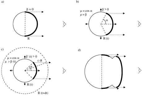
Figure 29: Dependence of the radiation flux at a remote point of observation (on the right) on the dynamical characteristics of the observed envelope. The envelope region from which the radiation reaches the observer is highlighted by the heavy line for the following cases: the envelope is at rest (a), expands with a constant velocity $v=\beta c$ (b), and expands with acceleration (c). Panel (d) shows the equitemporal surface the radiation from some regions of which does not reach the observer due to the peculiar envelope dynamics.

The last constraint is most stringent and includes the previous constraints as special cases. Let us demonstrate this using the following example. For the dynamics of an expanding envelope with a linear increase in velocity, the propagation law can be written as $R/c=R_{0}+\beta_{0}t+at^{2}$, where $R_{0}$, $\beta_{0}$, and $a$ are constants. Generally, the analytical solution is cumbersome and cuts out certain intervals of angles from the flux integration. However, it is reduced to $\mu_{\mathrm{min}}=\beta_{0}+2at/c$ for $R_{0}=0$ and we can see that, in this case, the flux will be lower than that in the case of envelope motion with a constant velocity.

To demonstrate the peculiarities of the flux behavior at the point of observation, let us consider the effect of a flux decrease in the problem of an outburst of radiation on the envelope surface. This problem for an instantaneous outburst and an envelope at rest was solved by Imshennik, Nadezhin & Utrobin (1981). It is similar to the problem of a light echo from a nova outburst considered long ago by Couderc (1939), see also Barkov & Bisnovatyi-Kogan (2005) for an infrared outburst generated by a gamma-ray burst in a dust cloud. In contrast, we investigate the influence of an outburst with duration $dt$ followed by envelope expansion on the radiation flux at the point of observation; the source cannot be considered stationary and instantaneous and the envelope motion can be relativistic.

Consider a spherical envelope with radius $R_{0}=c$ on the surface of which an outburst with intensity $I_{\nu}=100I_{\nu,0}$ and duration $dt=0.1$ s occurred at $t=0$ followed by envelope expansion according to the law $R=R_{0}+0.5c(t-dt)$. The calculated radiation flux from the envelope at a remote point of observation is shown in Fig. 30 (scenario $1$). Also shown here is a comparison with the flux calculated for the case where only the outburst without subsequent motion occurred on the envelope surface (scenario $2$) and the flux calculated when there was no outburst but the expansion followed (scenario $3$). The gentler flux decline in the first scenario than that in the second one stems from the fact that the flux from the envelope starting to move at $t=0.1$ s is higher that from the envelope at rest. The steep decline near $t=0.6$ s is related to the fact that the light from the moving parts of the envelope arrives at the point of observation earlier than that from the parts at rest and by $t=0.8$ s the moving parts completely obscure the delayed flux of the outburst from the envelope edges and the flux behavior begins to follow scenario $3$.

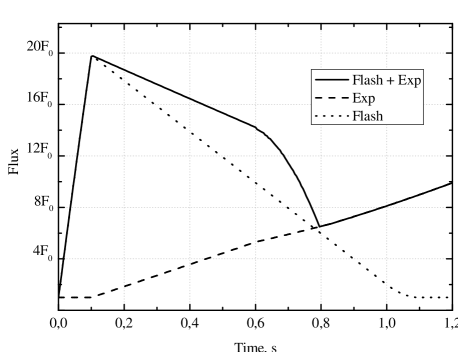
Figure 30: Radiation flux at a remote point of observation from an envelope of radius $R_{0}=c$ on the surface of which an outburst with intensity $I_{\nu}=100I_{\nu,0}$ and duration $dt=0.1R_{0}/c$ s occurred at $t=0$ followed by envelope expansion $R=R_{0}+0.5c(t-dt)$ (scenario 1). The dotted line denotes the flux as if only the outburst without any subsequent expansion occurred (scenario 2) and the dashed line represents only the motion (scenario 3). A zero time of observation corresponds to the outburst onset; $F_{0}$ is the radiation flux at a remote point of observation at the initial time $t=0$.

References

- Band et al. (2008) Band D. L., Grindlay J. E., Hong J., Fishman G., Hartmann D. H., Garson III A., Krawczynski H., Barthelmy S., Gehrels N., Skinner G., 2008, ApJ, 673, 1225
- Barkov & Bisnovatyi-Kogan (2005) Barkov M. V., Bisnovatyi-Kogan G. S., 2005, Astrophysics, 48, 369
- Becker (1988) Becker P. A., 1988, ApJ, 327, 772
- Belokon (1959) Belokon V. A., 1959, Soviet Physics – JETP, 9, 235
- Bisnovatyi-Kogan et al. (1975) Bisnovatyi-Kogan G. S., Imshennik V. S., Nadyozhin D. K., Chechetkin V. M., 1975, Ap&SS, 35, 23
- Blandford & Payne (1981a) Blandford R. D., Payne D. G., 1981a, MNRAS, 194, 1041
- Blandford & Payne (1981b) Blandford R. D., Payne D. G., 1981b, MNRAS, 194, 1033
- Blinnikov et al. (2003) Blinnikov S., Chugai N., Lundqvist P., Nadyozhin D., Woosley S., Sorokina E., 2003, in W. Hillebrandt & B. Leibundgut ed., From Twilight to Highlight: The Physics of Supernovae Observable Effects of Shocks in Compact and Extended Presupernovae. p. 23
- Blinnikov et al. (2000) Blinnikov S., Lundqvist P., Bartunov O., Nomoto K., Iwamoto K., 2000, ApJ, 532, 1132
- Blinnikov (1999) Blinnikov S. I., 1999, Astronomy Letters, 25, 359
- Blinnikov et al. (1998) Blinnikov S. I., Eastman R., Bartunov O. S., Popolitov V. A., Woosley S. E., 1998, ApJ, 496, 454
- Blinnikov et al. (2002) Blinnikov S. I., Nadyozhin D. K., Woosley S. E., Sorokina E. I., 2002, in W. Hillebrandt & E. Müller ed., Nuclear Astrophysics Shock breakouts in SNe Ib/c. pp 144–147
- Blinnikov et al. (2006) Blinnikov S. I., Röpke F. K., Sorokina E. I., Gieseler M., Reinecke M., Travaglio C., Hillebrandt W., Stritzinger M., 2006, A&A, 453, 229
- Blinnikov & Tolstov (2011) Blinnikov S. I., Tolstov A. G., 2011, Astronomy Letters, 37, 194
- Calzavara & Matzner (2004) Calzavara A. J., Matzner C. D., 2004, MNRAS, 351, 694
- Castor (1972) Castor J. I., 1972, ApJ, 178, 779
- Chevalier (1981) Chevalier R. A., 1981, Fundamentals of Cosmic Physics, 7, 1
- Colgate (1974) Colgate S. A., 1974, ApJ, 187, 333
- Colgate et al. (1972) Colgate S. A., McKee C. R., Blevins B. A., 1972, in Bulletin of the American Astronomical Society Vol. 4 of Bulletin of the American Astronomical Society, Relativistic shock propagation and search for supernova electromagnetic pulses.. p. 258
- Couderc (1939) Couderc P., 1939, Annales d’Astrophysique, 2, 271
- Dwek & Arendt (2008) Dwek E., Arendt R. G., 2008, ApJ, 685, 976
- Ensman & Burrows (1992) Ensman L., Burrows A., 1992, ApJ, 393, 742
- Fukue et al. (1985) Fukue J., Kato S., Matsumoto R., 1985, PASJ, 37, 383
- Gandelman & Frank-Kamenetsky (1956) Gandelman G. M., Frank-Kamenetsky D. A., 1956, Doklady Akad. Nauk SSSR, 107, 811
- Gezari et al. (2008) Gezari S., Dessart L., Basa S., Martin D. C., Neill J. D., Woosley S. E., Hillier D. J., Bazin G., Forster K., Friedman P. G., Le Du J., Mazure A., Morrissey P., Neff S. G., Schiminovich D., Wyder T. K., 2008, ApJL, 683, L131
- Grasberg (1981) Grasberg E. K., 1981, SvA, 25, 85
- Grassberg et al. (1971) Grassberg E. K., Imshennik V. S., Nadyozhin D. K., 1971, Ap&SS, 10, 28
- Grindlay et al. (2003) Grindlay J. E., Craig W. W., Gehrels N. A., Harrison F. A., Hong J., 2003, in J. E. Truemper & H. D. Tananbaum ed., Society of Photo-Optical Instrumentation Engineers (SPIE) Conference Series Vol. 4851 of Society of Photo-Optical Instrumentation Engineers (SPIE) Conference Series, EXIST: mission design concept and technology program. pp 331–344