Transverse spin gradient functional for non-collinear
spin density functional theory

Abstract

We present a novel functional for spin density functional theory aiming at the description of non-collinear magnetic structures. The construction of the functional employs the spin-spiral-wave state of the uniform electron gas as reference system. We show that the functional depends on transverse gradients of the spin magnetization, i.e. , in contrast to the widely used local spin density approximation, the functional is sensitive to local changes of the direction of the spin magnetization. As a consequence the exchange-correlation magnetic field is not parallel to the spin magnetization and a local spin-torque is present in the ground state of the Kohn-Sham system. As a proof-of-principle we apply the functional to a Chromium mono-layer in the non-collinear ${120^{\circ}}$-Néel state.

Since the discovery of the giant magnetoresistanceBaibich et al. (1988); *Grunberg:89 the field of spintronics Žutić et al. (2004) plays an important role in the everlasting goal to miniaturize devices for data storage and manipulation. For instance, the coupling of orbital and spin degrees of freedom is used to move magnetic domain walls in so-called “racetrack” memory devices Parkin et al. (2008) via a charge current. Similarly, spin polarized currents can switch the magnetic state of spin-valves by means of the so-called spin-transfer torque.Ralph and Stiles (2008) Whenever spin-orbit coupling is present, there is no global spin-quantization axis and the spin magnetization becomes non-collinear. A specific example of non-collinear magnetic structures on the nano scale are skyrmions Skyrme (1962), i.e. , topological twists in the spin magnetization, which recently have been observed in magnetic solids Mühlbauer et al. (2009) and magnetic surfaces.Heinze et al. (2011) Even within a single atom non-collinear magnetism is present.Nordström and Singh (1996); *EschrigServedio:99

Density functional theory (DFT) Dreizler and Gross (1990) is presently the most widely used approach to determine the electronic structure of large molecules and solids. Shortly after the original formulation by Hohenberg and Kohn Hohenberg and Kohn (1964) in terms of the electronic density ${n\left(\bm{r}\right)}$ alone, the theory was extended to include also the spin magnetization ${\bm{m}\!\left(\bm{r}\right)}$ as fundamental variable.von Barth and Hedin (1972) Spin density functional theory (SDFT) applies to Hamiltonians of the form

$$\hat{\mathcal{H}}=\hat{\mathcal{T}}+\hat{\mathcal{V}}+\hat{\mathcal{B}}+\hat{\mathcal{W}},$$ (1)

where in addition to the kinetic energy ${\hat{\mathcal{T}}}$, the potential energy ${\hat{\mathcal{V}}}$ and the electron-electron interaction energy ${\hat{\mathcal{W}}}$ a contribution, ${\hat{\mathcal{B}}}$, due to an external magnetic field ${\bm{B}\!\left(\bm{r}\right)}$ is considered, i.e. ,

$$\hat{\mathcal{B}}=-\mu_{\mathrm{B}}\int\!\!\mathrm{d}^{3}r\;\bm{B}\!\left(\bm{r}\right)\cdot\hat{\bm{m}}\!\left(\bm{r}\right).$$ (2)

The operator ${\hat{\bm{m}}\!\left(\bm{r}\right)=\hat{\Phi}^{\dagger}\!\left(\bm{r}\right)\bm{\sigma}\hat{\Phi}\!\left(\bm{r}\right)}$, representing the spin magnetization, is defined in terms of the spinor field ${\hat{\Phi}^{\dagger}\!\left(\bm{r}\right)=\begin{pmatrix}\hat{\phi}_{\uparrow}^{\dagger}\!\left(\bm{r}\right)&\hat{\phi}_{\downarrow}^{\dagger}\!\left(\bm{r}\right)\end{pmatrix}}$ and the vector of Pauli matrices ${\bm{\sigma}}$.

An immediate application of spin density functional theory (SDFT) is to find the configuration of the spin magnetization which is lowest in energy and hence the most stable. Furthermore it is possible to shape the spin magnetization via an external magnetic field. Comparing energies for different magnetic configurations (or equivalently different external magnetic fields) one can map out the energy landscape for a given material. A specific example is to constrain the spin magnetization to rotate in space with a given wave vector ${\bm{q}}$ in order to compute the magnon dispersion by ${\epsilon_{mag}\!\left(\bm{q}\right)=E\!\left(\bm{q}\right)-E\!\left(0\right)}$ (frozen magnon approach).

As always in DFTs the success of the theory hinges on the availability of accurate and physically sound approximations to the exchange-correlation (${xc}$) energy ${E_{xc}\!\left[n,\bm{m}\right]}$ - a functional of ${n\!\left(\bm{r}\right)}$ and ${\bm{m}\!\left(\bm{r}\right)}$ in the case of SDFT. The functional derivative of ${E_{xc}\!\left[n,\bm{m}\right]}$ w.r.t. the density (spin magnetization) yields the so-called ${xc}$ potential ${v_{xc}\!\left(\bm{r}\right)}$ (${xc}$ magnetic field ${\bm{B}_{xc}\!\left(\bm{r}\right)}$). These ${xc}$ potentials describe the effect of exchange and correlation in the Kohn-Sham (KS) system Kohn and Sham (1965), an effective system of non-interacting electrons, exposed to the potential ${v_{s}\!\left(\bm{r}\right)=v\!\left(\bm{r}\right)+v_{\mathrm{H}}\!\left(\bm{r}\right)+v_{xc}\!\left(\bm{r}\right)}$ and magnetic field ${\bm{B}_{s}\!\left(\bm{r}\right)=\bm{B}\!\left(\bm{r}\right)+\bm{B}_{xc}\!\left(\bm{r}\right)}$, which reproduces the density and spin magnetization of the interacting system.

The simplest approximation in the framework of DFT is the local density approximation (LDA) Kohn and Sham (1965), which determines the ${xc}$ energy of the non-uniform systems by treating it locally as a uniform electron gas. Including the spin magnetization this idea is readily generalized yielding for the ${xc}$ energy

$$E_{xc}^{\mathrm{LSDA}}\!\left[n,\bm{m}\right]=\int\!\!\mathrm{d}^{3}r\;n\!\left(\bm{r}\right)\varepsilon_{xc}^{\mathrm{unif}}\!\left(n\!\left(\bm{r}\right),m\!\left(\bm{r}\right)\right),$$ (3)

the so-called local spin density approximation (LSDA), with ${m\!\left(\bm{r}\right)}$ being the magnitude of ${\bm{m}\!\left(\bm{r}\right)}$ and ${\varepsilon_{xc}^{\mathrm{unif}}}$ the ${xc}$ energy of a spin-polarized uniform electron gas (UEG). For collinear magnetism, i.e. , ${\bm{m}\!\left(\bm{r}\right)}$ pointing in the same direction everywhere in space, a plethora of functionals was derived (cf. Ref. Rappoport et al., 2009) improving over the collinear LSDA, however, much less is known about constructing functionals for non-collinear magnetism, where the direction of ${\bm{m}\!\left(\bm{r}\right)}$ is allowed to vary freely in space. In fact, most applications of non-collinear SDFT up-to-date are based on the idea, pioneered by Kübler et al. Kübler et al. (1988), to apply collinear functionals to non-collinear systems by evaluating the functional in a local reference frame with the local ${z}$-axis determined by the direction of ${\bm{m}\!\left(\bm{r}\right)}$. The LSDA, defined in Eq. (3), employs a local reference frame intrinsically which can be seen by evaluating the corresponding ${xc}$ magnetic field

$$\bm{B}_{xc}^{\mathrm{LSDA}}\!\left(\bm{r}\right)=-\frac{\delta E_{xc}^{\mathrm{LSDA}}\!\left[n,\bm{m}\right]}{\delta\mu_{\mathrm{B}}\bm{m}\!\left(\bm{r}\right)}=-\frac{\partial\varepsilon_{xc}^{\mathrm{unif}}}{\partial m}\frac{n\!\left(\bm{r}\right)\bm{m}\!\left(\bm{r}\right)}{\mu_{\mathrm{B}}m\!\left(\bm{r}\right)}.$$ (4)

By construction ${\bm{B}_{xc}^{\mathrm{LSDA}}}$ is always aligned with ${\bm{m}}$. The same is true for generalized gradient approximations (GGAs) employing the aforementioned rotation to a local reference frame. In recent years attempts were made to extend GGAs and meta-GGAs to non-collinear systems without invoking a local reference frame in order to produce a ${\bm{B}_{xc}\!\left(\bm{r}\right)}$ which is non-collinear w.r.t. ${\bm{m}\!\left(\bm{r}\right)}$.Peralta et al. (2007); *ScalmaniFrisch:12 Since collinear functionals are usually formulated in terms of ${n_{\uparrow}\!\left(\bm{r}\right)}$ and ${n_{\downarrow}\!\left(\bm{r}\right)}$ (as opposed to ${n\!\left(\bm{r}\right)}$ and ${m\!\left(\bm{r}\right)}$) and gradients thereof, these approaches require a prescription mapping the gradient of ${\bm{m}\!\left(\bm{r}\right)}$ (a ${3\!\times\!3}$-matrix for non-collinear systems) to gradients of ${n_{\uparrow}\!\left(\bm{r}\right)}$ and ${n_{\downarrow}\!\left(\bm{r}\right)}$. Sharma et al. demonstrated that orbital functionals yield in general a ${\bm{B}_{xc}}$ which is non-collinear w.r.t. ${\bm{m}}$.Sharma et al. (2007) Another approach was to consider the variations of the direction of ${\bm{m}\!\left(\bm{r}\right)}$ perturbatively.Katsnelson and Antropov (2003); Capelle and Gyorffy (2003) Capelle and Oliveira proposed a non-local DFT approach Capelle and Oliveira (2000a, b), in close analogy to the DFT for superconductors.Oliveira et al. (1988)

In this letter we show that the very idea of the LSDA can be extended in a non-perturbative way to yield a new functional for SDFT depending on transverse gradients. This means that the ${xc}$ functional depends on spatial variations of the direction of ${\bm{m}}$ and, as a consequence, the ${xc}$ magnetic field exerts a local torque on the spin magnetization. This local torque is important for the ab-initio description of spin dynamics. Capelle et al. (2001)

In the LSDA the spin polarized UEG is chosen as reference system to determine the local ${xc}$ energy. Note that the LSDA does not employ the ground-state ${xc}$ energy of the UEG, but instead the minimal ${xc}$ energy of the UEG under the constraint that its spin magnetization is ${m_{0}}$. Usually one imposes the constraint of a fixed spin magnetization via a uniform magnetic field. The new functional is based on the idea to consider a reference system with a non-collinear spin magnetization. In close analogy to the LSDA the local ${xc}$ energy is determined from the UEG constrained to be in the so-called spin-spiral-wave (SSW) state.Overhauser (1962); *GiulianiVignaleSDW:05 The SSW state of the UEG is characterized by a constant density ${n_{0}}$ and a spin magnetization of the form

$$\bm{m}_{0}\!\left(\bm{r}\right)=m_{0}\begin{pmatrix}s\cos\!\left(\bm{q}\!\cdot\!\bm{r}\right)\\ s\sin\!\left(\bm{q}\!\cdot\!\bm{r}\right)\\ \sqrt{1-s^{2}}\end{pmatrix},$$ (5)

with ${s=\sin\!\left(\theta\right)}$ and ${\theta}$ is the azimuthal angle between the rotating part (in the ${x}$-${y}$ plane) and the constant part (parallel to ${z}$-axis). Similar to the case of the uniformly polarized UEG the constraint of a spin-spiral magnetization is imposed via a local external magnetic field that itself has a spiral structure. The ${xc}$ energy of the SSW UEG depends on four parameters: ${n_{0}}$, ${m_{0}}$, ${s}$ and ${q=|\bm{q}|}$. As we will see below it is possible to define local ${s\!\left(\bm{r}\right)}$ and ${q\!\left(\bm{r}\right)}$ in terms of transverse gradients of ${\bm{m}\!\left(\bm{r}\right)}$ which leads to the definition of the SSW functional

$$E_{xc}^{\mathrm{SSW}}\!\left[n,\bm{m}\right]=\int\!\!\mathrm{d}^{3}r\;n\!\left(\bm{r}\right)\varepsilon_{xc}^{\mathrm{SSW}}\!\left(n\!\left(\bm{r}\right),m\!\left(\bm{r}\right),s\!\left(\bm{r}\right),q\!\left(\bm{r}\right)\right),$$ (6)

where ${\varepsilon_{xc}^{\mathrm{SSW}}\!\left(n,m,s,q\right)}$ is the minimal ${xc}$ energy of the UEG under the constraint that it is in the SSW state specified by ${n}$, ${m}$, ${s}$ and ${q}$. It is important to realize that the LSDA is included in this definition in the limits ${s\to 0}$ or ${q\to 0}$, i.e. , $\varepsilon_{xc}^{\mathrm{SSW}}\!\left(n,m,s,q=0\right)=\varepsilon_{xc}^{\mathrm{SSW}}\!\left(n,m,s=0,q\right)=\varepsilon_{xc}^{\mathrm{SSW}}\!\left(n,m,s=0,q=0\right)=\varepsilon_{xc}^{\mathrm{unif}}\!\left(n,m\right)$. This can be emphasized by rewriting the SSW functional as

$$E_{xc}^{\mathrm{SSW}}\!\left[n,\bm{m}\right] =\int\!\!\mathrm{d}^{3}r\;n\!\left(\bm{r}\right)\varepsilon_{xc}^{\mathrm{unif}}\!\left(n\!\left(\bm{r}\right),m\!\left(\bm{r}\right)\right)$$

$$\times\left(1+S_{xc}\!\left(n\!\left(\bm{r}\right),m\!\left(\bm{r}\right),s\!\left(\bm{r}\right),q\!\left(\bm{r}\right)\right)\right),$$ (7)

where we have introduced the spin gradient enhancement (SGE)

$$S_{xc}\!\left(n,m,s,q\right)=\frac{\varepsilon_{xc}^{\mathrm{SSW}}\!\left(n,m,s,q\right)-\varepsilon_{xc}^{\mathrm{unif}}\!\left(n,m\right)}{\varepsilon_{xc}^{\mathrm{unif}}\!\left(n,m\right)}.$$ (8)

Before we discuss the explicit form of the local ${s\!\left(\bm{r}\right)}$ and ${q\!\left(\bm{r}\right)}$ we briefly discuss global, i.e. , spatially independent, rotations of the internal (spin) space. These rotations correspond to transforming ${\hat{\Phi}\!\left(\bm{r}\right)\to\mathcal{U}\hat{\Phi}\!\left(\bm{r}\right)}$, where ${\mathcal{U}}$ is an element of ${\mathrm{SU}\!\left(2\right)}$ (a rotation of the internal [spin] degree of freedom). Note that spatial vectors, e.g. the (charge) current ${\bm{\jmath}\!\left(\bm{r}\right)}$, are invariant under such internal rotations whereas spin vectors as ${\bm{m}\!\left(\bm{r}\right)}$ transform as ${\bm{m}\!\left(\bm{r}\right)\to\underline{R}\bm{m}\!\left(\bm{r}\right)}$, with ${\underline{R}}$ being the ${3\!\times\!3}$ rotation matrix corresponding to ${\mathcal{U}}$. Since the kinetic energy ${\hat{\mathcal{T}}}$ and the interaction energy ${\hat{\mathcal{W}}}$ are invariant under global rotations of the internal space it follows that ${E_{xc}\!\left[n,\bm{m}\right]=E_{xc}\!\left[n,\underline{R}\bm{m}\right]}$. Considering infinitesimal spin rotations one obtains the so-called zero-torque theorem

$$0=\int\!\!\mathrm{d}^{3}r\;\bm{m}\!\left(\bm{r}\right)\times\bm{B}_{xc}\!\left(\bm{r}\right),$$ (9)

which was first derived by Capelle et al. via the equation of motion for the spin magnetization.Capelle et al. (2001) It states that ${\bm{B}_{xc}}$ cannot exert a net torque on the whole system.

A simple rule to follow in order to ensure that explicit functionals for SDFT obey the zero-torque theorem is to write ${E_{xc}\!\left[n,\bm{m}\right]}$ in terms of proper scalars, i.e. , spin indices have to be contracted with spin indices and spatial indices with spatial indices. This implies that the determination of the local ${xc}$ energy in terms of strictly local densities is exhausted by ${n\!\left(\bm{r}\right)}$ and ${m\!\left(\bm{r}\right)}$. Hence the local ${s\!\left(\bm{r}\right)}$ and ${q\!\left(\bm{r}\right)}$ have to be determined from properly contracted gradients of ${\bm{m}\!\left(\bm{r}\right)}$.

Let us first look at ${D\!\left(\bm{r}\right)=|\nabla\!\otimes\!\bm{m}\!\left(\bm{r}\right)|^{2}}$, which corresponds to the total first order change of ${\bm{m}\!\left(\bm{r}\right)}$. It can be split into a longitudinal contribution ${D_{\mathrm{L}}\!\left(\bm{r}\right)}$ and a transverse contribution ${D_{\mathrm{T}}\!\left(\bm{r}\right)}$, i.e. ,

$$D\!\left(\bm{r}\right) =\frac{1}{m^{2}\!\left(\bm{r}\right)}\left(D_{\mathrm{L}}\!\left(\bm{r}\right)+D_{\mathrm{T}}\!\left(\bm{r}\right)\right),$$ (10)

$$D_{\mathrm{L}}\!\left(\bm{r}\right) =|\bm{m}\!\left(\bm{r}\right)\!\cdot\!\left(\nabla\!\otimes\!\bm{m}\!\left(\bm{r}\right)\right)|^{2},$$ (11)

$$D_{\mathrm{T}}\!\left(\bm{r}\right) =|\bm{m}\!\left(\bm{r}\right)\!\times\!\left(\nabla\!\otimes\!\bm{m}\!\left(\bm{r}\right)\right)|^{2},$$ (12)

where the meaning of longitudinal and transverse is defined by the local direction of ${\bm{m}\!\left(\bm{r}\right)}$. We use “${\otimes}$” to emphasize that the gradient of the magnetization is a tensor. The scalar and the cross product in Eqs. (11) and (12) act on the components of ${\bm{m}}$. For the SSW UEG the two contributions are ${D_{\mathrm{L}}^{\mathrm{SSW}}=0}$ and ${D_{\mathrm{T}}^{\mathrm{SSW}}=m_{0}^{4}s^{2}q^{2}}$. Both contributions are constant in space for the SSW UEG and hence play a similar role as the density ${n_{0}}$ and the magnitude of the spin magnetization ${m_{0}}$, i.e. , they locally characterize the state. ${D_{\mathrm{L}}^{\mathrm{SSW}}}$ vanishes because the spin magnetization in the SSW UEG only rotates (the magnitude ${m}$ is constant). ${D_{\mathrm{T}}}$ does not vanish but it only determines the combination ${sq}$.

Accordingly we look at the second order variation ${d\!\left(\bm{r}\right)=|\nabla^{2}\bm{m}\!\left(\bm{r}\right)|^{2}}$. Again, it can be analyzed w.r.t. longitudinal and transverse contributions

$$d\!\left(\bm{r}\right) =\frac{1}{m^{2}\!\left(\bm{r}\right)}\left(d_{\mathrm{L}}\!\left(\bm{r}\right)+d_{\mathrm{T}}\!\left(\bm{r}\right)\right),$$ (13)

$$d_{\mathrm{L}}\!\left(\bm{r}\right) =|\bm{m}\!\left(\bm{r}\right)\!\cdot\!\left(\nabla^{2}\bm{m}\!\left(\bm{r}\right)\right)|^{2},$$ (14)

$$d_{\mathrm{T}}\!\left(\bm{r}\right) =|\bm{m}\!\left(\bm{r}\right)\!\times\!\left(\nabla^{2}\bm{m}\!\left(\bm{r}\right)\right)|^{2}.$$ (15)

For our reference system this yields ${d_{\mathrm{L}}^{\mathrm{SSW}}=m_{0}^{4}s^{4}q^{4}}$ and ${d_{\mathrm{T}}^{\mathrm{SSW}}=m_{0}^{4}\left(1-s^{2}\right)s^{2}q^{4}}$. The change of ${\bm{m}\!\left(\bm{r}\right)}$ to first order is perpendicular to ${\bm{m}\!\left(\bm{r}\right)}$, but to second order ${\bm{m}\!\left(\bm{r}\right)}$ also changes in the direction of ${\bm{m}\!\left(\bm{r}\right)}$ which explains why ${d_{\mathrm{L}}^{\mathrm{SSW}}}$ does not vanish for the SSW UEG. However, we see that ${d_{\mathrm{L}}^{\mathrm{SSW}}}$ provides the same information as ${D_{\mathrm{T}}^{\mathrm{SSW}}}$, meaning, ${sq}$ to some power. Adopting the strategy that we obtain the characteristic parameters for the local ${xc}$ energy choosing the order of derivatives as low as possible, ${s\!\left(\bm{r}\right)}$ and ${q\!\left(\bm{r}\right)}$ are given by

$$s\!\left(\bm{r}\right) =\sqrt{\frac{D_{\mathrm{T}}^{2}\!\left(\bm{r}\right)}{D_{\mathrm{T}}^{2}\!\left(\bm{r}\right)+m^{4}\!\left(\bm{r}\right)d_{\mathrm{T}}\!\left(\bm{r}\right)}},$$ (16)

$$q\!\left(\bm{r}\right) =\sqrt{\frac{D_{\mathrm{T}}^{2}\!\left(\bm{r}\right)+m^{4}\!\left(\bm{r}\right)d_{\mathrm{T}}\!\left(\bm{r}\right)}{m^{4}\!\left(\bm{r}\right)D_{\mathrm{T}}\!\left(\bm{r}\right)}}.$$ (17)

This completes the definition of the SSW functional Eq. (6) or equivalently the SGE to the LSDA Eq. (7).

By definition (c.f. Eq. (16)) the local ${s\!\left(\bm{r}\right)}$ is between ${\left[0,1\right]}$ in accordance with being the sine of an azimuthal angle. Furthermore we have the following hierarchy in the dependence of the SGE, Eq. (7), on the transverse gradients: i) If ${D_{\mathrm{T}}\!\left(\bm{r}\right)=0}$, the SGE correction is zero. ii) If ${D_{\mathrm{T}}\!\left(\bm{r}\right)\neq 0}$ and ${d_{\mathrm{T}}\!\left(\bm{r}\right)=0}$, the SGE correction is obtained from a planar SSW (${s=1}$). iii) If both transverse gradients are non-zero the SGE correction is obtained from a general SSW.

We proceed by evaluating the ${xc}$ magnetic field from the SSW functional,

$$\bm{B}_{xc}^{\mathrm{SSW}}\!\left(\bm{r}\right)=-\frac{\delta E_{xc}\!\left[n,\bm{m}\right]}{\delta\mu_{\mathrm{B}}\bm{m}\!\left(\bm{r}\right)}=\bm{B}_{xc}^{m}+\bm{B}_{xc}^{D_{\mathrm{T}}}+\bm{B}_{xc}^{d_{\mathrm{T}}},$$ (18)

where we split ${\bm{B}_{xc}^{\mathrm{SSW}}\!\left(\bm{r}\right)}$ into contributions coming from the dependence of ${\varepsilon_{xc}^{\mathrm{SSW}}}$ on ${m}$, ${D_{\mathrm{T}}}$ and ${d_{\mathrm{T}}}$, respectively. The explicit evaluation of ${\bm{B}_{xc}^{\mathrm{SSW}}\!\left(\bm{r}\right)}$ is straight-forward but rather lengthy. Here we will show the energetic content in the KS system, i.e. ,

$$E_{\bm{B}_{xc}}^{\mathrm{KS}}=-\mu_{\mathrm{B}}\int\!\!\mathrm{d}^{3}r\;\bm{m}\!\left(\bm{r}\right)\!\cdot\!\bm{B}_{xc}\!\left(\bm{r}\right)$$

$$=2\int\!\!\mathrm{d}^{3}r\;n\!\left(\bm{r}\right)\left(\partial_{m^{2}}\varepsilon_{xc}^{\mathrm{SSW}}\right)|\bm{m}\!\left(\bm{r}\right)|^{2}$$ (19)

$$+4\int\!\!\mathrm{d}^{3}r\;n\!\left(\bm{r}\right)\left(\partial_{D_{\mathrm{T}}}\varepsilon_{xc}^{\mathrm{SSW}}\right)|\bm{m}\!\left(\bm{r}\right)\!\times\!\left(\nabla\!\otimes\!\bm{m}\!\left(\bm{r}\right)\right)|^{2}$$ (20)

$$+4\int\!\!\mathrm{d}^{3}r\;n\!\left(\bm{r}\right)\left(\partial_{d_{\mathrm{T}}}\varepsilon_{xc}^{\mathrm{SSW}}\right)|\bm{m}\!\left(\bm{r}\right)\!\times\!\left(\nabla^{2}\bm{m}\!\left(\bm{r}\right)\right)|^{2}.$$ (21)

The first term (Eq. (19)) is already present in the LSDA, whereas the other two terms (Eqs. (20),(21)) arise due to the inclusion of the SGE. The zero-torque theorem, Eq. (9), is fulfilled by construction, however the new terms in ${\bm{B}_{xc}\!\left(\bm{r}\right)}$ are non-collinear w.r.t. ${\bm{m}\!\left(\bm{r}\right)}$, i.e. , they provide a local torque.

The final step for a practical implementation of the SSW functional is the determination of the SGE from the SSW UEG. We have evaluated ${S_{xc}\!\left(n,m,s,q\right)}$ using the random-phase approximation (RPA) for the SSW UEG. It is important to stress that we approximate the ${S_{xc}}$ with the RPA and not ${\varepsilon_{xc}^{\mathrm{SSW}}}$. In this way the SSW functional reduces to the LSDA parameterized using the Monte Carlo reference data.Ceperley and Alder (1980); *PerdewWang:92 From ${\sim 65000}$ data points in the four-dimensional domain of ${S_{xc}}$ we have constructed a polynomial fit for ${S_{xc}}$.

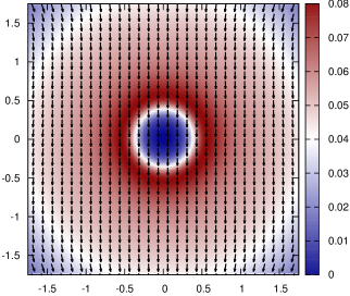
Figure 1: (Color online). Magnitude (color coded) and direction (arrows) of ${\bm{B}_{xc}\!\left(\bm{r}\right)}$ around an atom for the Cr mono-layer using the LSDA.

As a first application we have implemented the SSW functional in the ELK code ELK in order to investigate the Chromium mono-layer in the ${120^{\circ}}$-Néel state. In FIGs. 1 and 2 we plot the magnitude and direction of ${\bm{B}_{xc}}$ in order to illustrate the qualitative difference between the LSDA and the SSW functional. While the local spin magnetizations ${\bm{m}\!\left(\bm{r}\right)}$ are similar for the LSDA and the SSW functional, ${\bm{B}_{xc}}$ obtained via the SGE exhibits much more structure compared to the LSDA ${\bm{B}_{xc}}$. As a result the local torque does not vanish and a ground-state spin current is present in the KS system. The local torque which is completely missed by the usual LSDA is shown explicitly in FIG. 3 for the non-collinear the ${120^{\circ}}$-Néel state. The global zero-torque theorem (cf. Eq. (9)) may be inferred from the pattern of negative (blue) and positive (red) local torques around the nuclei. Since the SSW functional is not restricted to small ${q\!\left(\bm{r}\right)}$ it accounts for the intra-atomic non-collinearity.

In conclusion we have proposed a novel functional for SDFT depending on the first and second order transverse gradients of ${\bm{m}\!\left(\bm{r}\right)}$. We emphasize that this functional is formulated in terms of an enhancement to the LSDA. In particular this means that the correction vanishes in the case of a collinear system. The construction of the new functional parallels closely the original formulation of the LSDA. On one hand this means that the system is locally treated as a uniform electron gas in the SSW state, which may appear as a rather crude approximation. On the other hand the success of DFT may be attributed, to some extent, to the fact that the LDA already represents a reasonable approximation even for strongly inhomogeneous systems. GGAs are also corrections to the LSDA, hence it is conceivable to employ the two corrections simultaneously. Since GGAs are constructed having collinear systems in mind, one may argue that the longitudinal gradients ${D_{\mathrm{L}}\!\left(\bm{r}\right)}$, ${d_{\mathrm{L}}\!\left(\bm{r}\right)}$ should enter in the GGA part. We expect that the SGE will improve the ab-initio description of materials exhibiting a non-collinear magnetic structure.

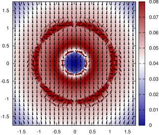
Figure 2: (Color online). Same as FIG. 1 for the SSW functional (LSDA+SGE). Note the richer structure of ${\bm{B}_{xc}\!\left(\bm{r}\right)}$ close to the Cr nucleus.

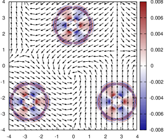
Figure 3: (Color online). The ${z}$-component of ${\bm{m}\!\left(\bm{r}\right)\!\times\!\bm{B}_{xc}\!\left(\bm{r}\right)}$ (color coded) around Cr atoms in the mono-layer computed using the SGE functional. The arrows show the direction of the spin magnetization.

While the corrections to the part of the ${\bm{B}_{xc}\!\left(\bm{r}\right)}$ parallel to ${\bm{m}\!\left(\bm{r}\right)}$ will adjust the energetics, the perpendicular part of ${\bm{B}_{xc}\!\left(\bm{r}\right)}$ describes the ${xc}$ corrections to the spin current, which in turn is crucial for ab-initio spin dynamics. We expect that the functional presented in this letter will pave the road to a better description of domain wall motion and spin wave propagation from first principles in the framework of time-dependent SDFT.

In both aforementioned scenarios it is important to have a numerically accessible functional which, given currently available computing facilities, implies the use of semi-local functionals. We have demonstrated that non-collinearity can be included by a generalization of the reference system employed in the LSDA and hence the numerical accessibility of the LSDA is retained in the SSW functional making it the ideal candidate for large scale quantum simulations.