Energy-Efficient Resource Allocation in Multiuser OFDM Systems with Wireless Information and Power Transfer

Abstract

In this paper, we study the resource allocation algorithm design for multiuser orthogonal frequency division multiplexing (OFDM) downlink systems with simultaneous wireless information and power transfer. The algorithm design is formulated as a non-convex optimization problem for maximizing the energy efficiency of data transmission (bit/Joule delivered to the users). In particular, the problem formulation takes into account the minimum required system data rate, heterogeneous minimum required power transfers to the users, and the circuit power consumption. Subsequently, by exploiting the method of time-sharing and the properties of nonlinear fractional programming, the considered non-convex optimization problem is solved using an efficient iterative resource allocation algorithm. For each iteration, the optimal power allocation and user selection solution are derived based on Lagrange dual decomposition. Simulation results illustrate that the proposed iterative resource allocation algorithm achieves the maximum energy efficiency of the system and reveal how energy efficiency, system capacity, and wireless power transfer benefit from the presence of multiple users in the system.

I Introduction

Orthogonal frequency division multiplexing (OFDM) is one of the leading candidates for supporting high data rate wireless broadband communication systems, as envisioned e.g. in the 3GPP Long Term Evolution Advanced (LTE-A) and IEEE 802.11 a/g/n Wireless Fidelity (Wi-Fi) standards, due to its flexibility in resource allocation and ability in exploiting multiuser diversity. In practice, a wireless communication system is expected to support multiple mobile users and to guarantee quality of service. However, because of the limited radio resources and harsh wireless channel conditions, some of the mobile users are typically switched to idle mode since they cannot be served by the system temporarily. Unfortunately, mobile devices are often battery driven and energy is dissipated even if they are idle which creates bottlenecks in perpetuating the network’s lifetime.

Recently, driven by environmental concerns, green mobile communication has received considerable interest from both industry and academia [1]-[3]. A promising approach to enhance the energy efficiency (bit-per-Joule) of wireless communication systems is to harvest energy from the environment. Solar, wind, and geothermal are the major renewable energy sources for generating electricity. However, these conventional natural energy sources may not be suitable for mobile devices and not be available in enclosed/indoor environments. On the other hand, wireless power transfer, in which energy is harvested from propagating electromagnetic waves (EM) in radio frequency (RF), is becoming a new paradigm in energy harvesting since it recycles the abundant ambient RF energy [4]–[9]. Although the development of wireless power transfer technology is still in its infancy, there have been some preliminary applications of wireless power transfer such as wireless body area networks (WBAN) for biomedical implants [4] and passive radio-frequency identification (RFID) systems [5]. Indeed, EM waves can carry both information and power/energy simultaneously [6]–[9]. The utilization of this characteristic of EM waves imposes many new challenges for wireless communication engineers. In [6] and [7], the fundamental trade-off between system capacity and wireless power transfer was studied for flat fading and frequency selective channels, respectively. However, [6] and [7] assumed a theoretical receiver, which is able to decode information and extract power from the same received signal but is not yet available in practice. In [8] and [9], the authors proposed different power allocation schemes for multiple antenna two-user narrowband systems by separating the process of information decoding and energy harvesting into two receivers. However, if a multicarrier system with an arbitrary number of users is considered, the results in [8] and [9] which are valid for single-carrier transmission, may no longer be applicable. Besides, the energy efficiency of wireless information and power transfer systems is still unknown since the power dissipations in RF transmission and electronic circuitries have not been taken into account in the literature, e.g. [6]–[9].

In this paper, we address the above issues and focus on the resource allocation algorithm design for energy efficient communication in multiuser OFDM systems with wireless information and power transfer. In Section II, we introduce the adopted multiuser OFDM channel model. In Section III, we formulate the resource allocation algorithm design as a non-convex optimization problem, which is solved by an efficient iterative resource allocation algorithm in Section IV. Section V presents simulation results for the system performance, and in Section VI, we conclude with a brief summary of our results.

II System Model

In this section, we introduce the OFDM system model.

II-A Multiuser OFDM Channel Model

We consider a multiuser OFDM system which consists of a transmitter and $K$ mobile users. All transceivers are equipped with a single antenna, cf. Figure 1. The total bandwidth of the system is $\cal B$ Hertz and there are $n_{F}$ subcarriers. Each subcarrier has a bandwidth $W={\cal B}/n_{F}$ Hertz. We assume that the OFDM signaling is time slotted and the length of each time (/scheduling) slot is comparable to the length of the channel coherence time; the channel impulse response is assumed to be time invariant during each scheduling slot. As a result, the downlink channel state information (CSI) can be accurately obtained by exploiting feedback from users in frequency division duplex (FDD) systems and channel reciprocity in time division duplex (TDD) systems. At the beginning of each scheduling slot, the transmitter computes the resource allocation policy based on the available CSI. The downlink received symbol at user $k\in\{1,\,\ldots,\,K\}$ on subcarrier $i\in\{1,\,\ldots,\,n_{F}\}$ in a scheduling slot is given by

$$Y_{i,k}=\sqrt{P_{i,k}l_{k}g_{k}}H_{i,k}X_{i,k}+Z_{i,k},$$ (1)

where $X_{i,k}$, $P_{i,k}$, and ${H}_{i,k}$ are the transmitted symbol, the transmitted power, and the multipath fading coefficient between the transmitter and user $k$ on subcarrier $i$, respectively. We assume that the transmitted symbol is zero mean with variance ${\cal E}\{\lvert X_{i,k}\rvert^{2}\}=1,\,\forall i,k,$ where ${\cal E}\{\cdot\}$ denotes statistical expectation. $l_{k}$ and $g_{k}$ represent the path loss and shadowing between the transmitter and user $k$, respectively. $Z_{i,k}$ is the additive white Gaussian noises (AWGN) on subcarrier $i$ at user $k$ with zero mean and variance $\sigma_{z}^{2}$.

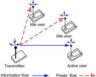
Figure 1: Illustration of a multiuser OFDM system with $K=3$ users for downlink wireless information and power transfer.

II-B Information Decoding and Energy Harvesting Receiver

In this paper, we assume that each user has the ability to decode the modulated information and to harvest energy from the received radio signal. However, the signal used for decoding of the modulated information cannot be used for harvesting energy [8]. As a result, at any given scheduling slot, a user can either decode information when it is active (being served by the transmitter) or harvest energy when it is idle, but not both concurrently, cf. Figure 1.

III Resource Allocation

In this section, we define the system energy efficiency and formulate the corresponding resource allocation problem.

III-A Instantaneous Channel Capacity

In this subsection, we define the adopted system performance measure. Given perfect CSI at the user, the channel capacity in a scheduling slot between the transmitter and user $k$ on subcarrier $i$ with channel bandwidth $W$ is given by

$$C_{i,k}=W\log_{2}\Big{(}1+P_{i,k}\Gamma_{i,k}\Big{)}\,\,\,\,\mbox{and}\,\,\,\,\Gamma_{i,k}=\frac{l_{k}g_{k}\lvert H_{i,k}\rvert^{2}}{\sigma_{z}^{2}},$$ (2)

where $\Gamma_{i,k}$ is the channel-to-noise ratio (CNR) at user $k$ on subcarrier $i$. On the other hand, we assume that in each scheduling slot one user is selected for information transfer and served by the transmitter. Concurrently, the remaining $K-1$ idle users harvest energy from the radio signal emitted by the transmitter. Then, the system capacity in a scheduling slot is defined as the total number of bits successfully delivered to the selected user (bit-per-second) and is given by

$$U({\cal P},{\cal S})=\sum_{i=1}^{n_{F}}\sum_{k=1}^{K}w_{k}s_{k}C_{i,k},$$ (3)

where ${\cal P}=\{P_{i,k}\geq 0,\,\forall i,k\}$ and ${\cal S}=\{s_{k}=\{0,1\},\forall k\}$ are the power allocation and user selection policies, respectively. $w_{k}\geq 0,\,\forall k,$ is a positive constant which allows the transmitter to give different priorities to different mobile users and to enforce certain notions of fairness. On the other hand, for designing an energy efficient resource allocation algorithm, we incorporate the total power dissipation of the system in the optimization objective function. To this end, we model the power dissipation (Joule-per-second) in the system as:

$$U_{TP}({\cal P},{\cal S}) = P_{C}+\sum_{i=1}^{n_{F}}\sum_{k=1}^{K}\varepsilon P_{i,k}s_{k}-P_{H}$$ (4)

$$\mbox{where}\,\,P_{H} = \underbrace{\sum_{i=1}^{n_{F}}\sum_{k=1}^{K}P_{i,k}s_{k}\Big{(}\sum_{j\neq k}\eta_{j}\lvert H_{i,j}\rvert^{2}l_{j}g_{j}\Big{)}}_{\mbox{Power harvested by idle users}}$$ (5)

and $j\in\{1,\,\ldots,\,K\}$. $P_{C}>0$ is the static circuit power dissipation of device electronics of the active transceiver such as mixers, filters, digital-to-analog converters, and is independent of the actual transmitted power. The total power consumption of the $K-1$ idle users is omitted in (4) since it is relatively small compared to the power dissipation of the active transceiver pair. The middle term on the right hand side of (4) is the power consumption in the power amplifier and $\varepsilon\geq 1$ is a constant which accounts for the power inefficiency of the power amplifier. For example, if $\varepsilon=5$, then $5$ Watts are consumed in the power amplifier for every 1 Watt of power radiated in the RF which results in a power efficiency of $\frac{1}{\varepsilon}=\frac{1}{5}=20\%$; power that is not converted to a useful signal is dissipated as heat in the power amplifier. On the other hand, the minus sign in front of $P_{H}$ in (4) indicates that a part of the power radiated by the transmitter can be possibly harvested by the idle users. Here, we assume that the ability to harvest energy is heterogeneous. Specifically, we define the constant parameter $0\leq\eta_{j}\leq 1$ used in (5) as user $j$’s efficiency in harvesting energy from the received radio signal. The term $\eta_{j}\lvert H_{i,j}\rvert^{2}l_{j}g_{j}$ in (5) can be interpreted as frequency selective power transfer efficiency for transferring power from the transmitter to idle user $j$ on subcarrier $i$. We note that although $U_{TP}({\cal P},{\cal S})$ can be a negative value mathematically since $\lvert H_{i,j}\rvert^{2}\in[0,\infty)$, $U_{TP}({\cal P},{\cal S})>0$ always holds in practical communication systems. In particular, since the transmitter is the only RF energy source of the idle users, we have $\sum_{i=1}^{n_{F}}\sum_{k=1}^{K}\varepsilon P_{i,k}s_{k}\geq\sum_{i=1}^{n_{F}}\sum_{k=1}^{K}P_{i,k}s_{k}\geq\sum_{i=1}^{n_{F}}\sum_{k=1}^{K}P_{i,k}s_{k}\Big{(}\sum_{j\neq k}\eta_{j}\lvert H_{i,j}\rvert^{2}l_{j}g_{j}\Big{)}$, where the second inequality is due to the second law of thermodynamics in energy flow from physic.

The energy efficiency of the considered system in a scheduling slot is defined as the total number of bits successfully delivered to the selected users per unit energy consumption (bit-per-Joule) which is given by

$$U_{eff}({\cal P},{\cal S}) = \frac{U({\cal P},{\cal S})}{U_{TP}({\cal P},{\cal S})}.$$ (6)

III-B Optimization Problem Formulation

The optimal power allocation policy, ${\cal P}^{*}$, and user selection policy, ${\cal S}^{*}$, can be obtained by solving

$$\hskip 42.67912pt\max_{{\cal P},{\cal S}}\,\,U_{eff}({\cal P},{\cal S})$$ (7)

s.t. $$\mbox{C1:}\,\,\sum_{i=1}^{n_{F}}\sum_{j=1}^{K}P_{i,j}s_{j}\Big{(}\eta_{k}\lvert H_{i,k}\rvert^{2}l_{k}g_{k}\Big{)}\geq(1-s_{k})P_{\min_{k}}^{req},\,\forall k,$$

$$\mbox{C2:}\,\,\sum_{i=1}^{n_{F}}\sum_{k=1}^{K}P_{i,k}s_{k}\leq P_{\max},$$

$$\mbox{C3:}\,\,\sum_{i=1}^{n_{F}}\sum_{k=1}^{K}\varepsilon P_{i,k}s_{k}+P_{C}\leq P_{PG},$$

$$\mbox{C4:}\,\,\sum_{i=1}^{n_{F}}\sum_{k=1}^{K}s_{k}C_{i,k}\geq R_{\min}\hskip 22.76219pt\mbox{C5:}\,\,\sum_{k=1}^{K}s_{k}\leq 1,$$

$$\mbox{C6:}\,\,s_{k}\in\{0,1\},\,\forall k,\hskip 50.07686pt\mbox{C7:}\,\,P_{i,k}\geq 0,\forall i,k.$$

Here, $P_{\min_{k}}^{req}$ in C1 denotes the minimum required power transfer for user $k$ if it is idle. $P_{\max}$ in C2 is the maximum transmit power allowance to control the amount of out-of-cell interference. C3 constrains the total power consumption of the system to not exceed the maximum power supply from the power grid, $P_{PG}$. C4 ensures a minimum required system data rate $R_{\min}$. C6 is a combinatorial constraint on the user selection variables. C5 and C6 are imposed to guarantee that in each scheduling slot at most one user is served by the transmitter. C7 is the non-negative constraint on the power allocation variables.

IV Solution of the Optimization Problem

The optimization problem in (7) is a mixed non-convex and combinatorial optimization problem. The non-convexity comes from the objective function which is the ratio of two functions and the combinatorial nature comes from the integer constraint for user selection. The first step in solving the considered problem is to simplify the objective function using techniques from nonlinear fractional programming.

IV-A Transformation of the Objective Function

For the sake of presentation simplicity, we define $\mathcal{F}$ as the set of feasible solutions of the optimization problem in (7) and $\{{\cal P},{\cal S}\}\in\mathcal{F}$. As the power allocation variables are constrained by C2, C3, and C7, $\mathcal{F}$ is a compact set. Without loss of generality, we define $q^{*}$ as the maximum energy efficiency of the considered system which is given by

$$q^{*}=\frac{U({\cal P^{*}},{\cal S^{*}})}{U_{TP}({\cal P^{*}},{\cal S^{*}})}=\max_{{\cal P},{\cal S}}\,\frac{U({\cal P},{\cal S})}{U_{TP}({\cal P},{\cal S})}.$$ (8)

We are now ready to introduce the following Theorem which is borrowed from nonlinear fractional programming [10].

Theorem 1

The maximum energy efficiency $q^{*}$ is achieved if and only if

$$\max_{{\cal P},{\cal S}} \,U({\cal P},{\cal S})-q^{*}U_{TP}({\cal P},{\cal S})$$

$$= U({\cal P^{*}},{\cal S^{*}})-q^{*}U_{TP}({\cal P^{*}},{\cal\cal S^{*}})=0,$$ (9)

for $U({\cal P},{\cal S})\geq 0$ and $U_{TP}({\cal P},{\cal S})>0$.

 Proof: Please refer to [3, Appendix A] for a proof of Theorem 1.

Theorem 1 provides a necessary and sufficient condition for the optimal resource allocation policy. Specifically, for an optimization problem with an objective function in fractional form, there exists an equivalent optimization problem with an objective function in subtractive form, e.g. $U({\cal P},{\cal S})-q^{*}U_{TP}({\cal P},{\cal S})$ in the considered case, such that both problem formulations lead to the same optimal resource allocation policy. As a result, we can focus on the equivalent objective function in the rest of the paper.

TABLE I: Iterative Resource Allocation Algorithm.

Algorithm 1 Iterative Resource Allocation Algorithm

1:  Initialize the maximum number of iterations $L_{max}$ and the maximum tolerance $\epsilon$

2:  Set maximum energy efficiency $q=0$ and iteration index $n=0$

3:  repeat {Main Loop}

4:     Solve the inner loop problem in (10) for a given $q$ and obtain resource allocation policy $\{{\cal P^{\prime}},{\cal S^{\prime}}\}$

5:     if $U({\cal P^{\prime}},{\cal S^{\prime}})-qU_{TP}({\cal P^{\prime}},{\cal S^{\prime}})<\epsilon$ then

6:        $\mbox{Convergence}=\,$true

7:        return  $\{{\cal P^{*},\cal S^{*}}\}=\{{\cal P^{\prime},\cal S^{\prime}}\}$ and $q^{*}=\frac{U({\cal P^{\prime}},{\cal S^{\prime}})}{U_{TP}({\cal P^{\prime}},{\cal S^{\prime}})}$

8:     else

9:        Set $q=\frac{U({\cal P^{\prime}},{\cal S^{\prime}})}{U_{TP}({\cal P^{\prime}},{\cal S^{\prime}})}$ and $n=n+1$

10:        Convergence $=$ false

11:     end if

12:  until Convergence $=$ true or $n=L_{max}$

IV-B Iterative Algorithm for Energy Efficiency Maximization

In this section, an iterative algorithm (known as the Dinkelbach method [10]) is proposed for solving (7) with an equivalent objective function such that the obtained resource allocation policy satisfies the conditions stated in Theorem 1. The proposed algorithm is summarized in Table I and the convergence to the maximum energy efficiency is guaranteed if the inner problem (10) in each iteration can be solved.

Proof: Please refer to [3, Appendix B] for a proof of convergence.

As shown in Table I, in each iteration in the main loop, i.e., in lines 3–12, we solve the following optimization problem for a given parameter $q$:

$$\max_{{\cal P},{\cal S}}\,\,\,{U}({\cal P},{\cal S})-q{U}_{TP}({\cal P},{\cal S})$$ (10)

$$\mbox{s.t.}\,\,\mbox{C1, C2, C3, C4, C5, C6, C7}.$$

We note that ${U}({\cal P},{\cal S})-q{U}_{TP}({\cal P},{\cal S})\geq 0$ holds for any value of $q$ generated by Algorithm I. Please refer to [3, Proposition 3] for a proof. On the other hand, it can be observed that the problem formulation in (10) for energy efficiency maximization is a generalized problem formulation for aggregate weighted system capacity maximization. Indeed, if we set $q=0$, then the objective function in (10) will become the aggregate weighted system capacity.

Solution of the Main Loop Problem

The transformed problem is now a mixed convex and combinatorial optimization problem. The integer constraint for user selection in C6 is still an obstacle in tackling the problem. Indeed, the traditional brute force approach or a branch-and-bound method can be used to obtain a global optimal solution but result in a prohibitively high complexity with respect to (w.r.t.) the numbers of users and subcarriers. In order to strike a balance between computational complexity and optimality, we follow the approach in [11] and relax $s_{k}$ in constraint C6 to be a real value between zero and one instead of a Boolean, i.e., $\mbox{C6: }0\leq s_{k}\leq 1,\,\forall k$. Then, $s_{k}$ can be interpreted as a time-sharing factor for the $K$ users to utilize the subcarriers. For facilitating the time-sharing, we introduce a new variable and define it as $\tilde{P}_{i,k}={P}_{i,k}s_{k},\,\forall i,k$. The variable represents the actual transmitted power in the RF of the transmitter on subcarrier $i$ for user $k$ under the time-sharing assumption. Although the relaxation of the user selection constraint will generally lead to a suboptimal solution, the authors in [12] show that the duality gap (suboptimality) due to the constraint relaxation becomes zero when the number of subcarriers is sufficiently large, e.g. $n_{F}=128$.

With this relaxation, it can be shown that the problem is now jointly concave w.r.t. the power allocation and user selection variables under the time-sharing assumption. As a result, under some mild conditions, solving the dual problem is equivalent to solving the primal problem [13].

IV-C Dual Problem Formulation

In this subsection, we solve the resource allocation optimization problem by solving its dual for a given value of $q$. For this purpose, we need the Lagrangian function of the primal problem in (10) which is given by

$${\cal L}(\boldmath\textbf{$\alpha$},\beta,\gamma,\lambda,\delta,{\cal P},{\cal S})$$

$$= \sum_{k=1}^{K}\sum_{i=1}^{n_{F}}(w_{k}+\gamma)s_{k}C_{i,k}-q\Big{(}U_{TP}({\cal P},{\cal S})\Big{)}$$

$$- \lambda\Big{(}\sum_{i=1}^{n_{F}}\sum_{k=1}^{K}\varepsilon\tilde{P}_{i,k}+P_{C}-P_{PG}\Big{)}-\delta\Big{(}\sum_{k=1}^{K}s_{k}-1\Big{)}$$

$$- \beta\Big{(}\sum_{i=1}^{n_{F}}\sum_{k=1}^{K}\tilde{P}_{i,k}s_{k}-P_{\max}\Big{)}-\gamma R_{\min}$$

$$- \sum_{k=1}^{K}\alpha_{k}\Big{(}(1-s_{k})P_{\min_{k}}^{req}-\sum_{i=1}^{n_{F}}\sum_{j=1}^{K}\tilde{P}_{i,j}\Big{(}\eta_{k}\lvert H_{i,k}\rvert^{2}l_{k}g_{k}\Big{)}\Big{)}.$$

Here, $\alpha$ has elements $\alpha_{k}$, $k\in\{1,\ldots,K\}$, and is the Lagrange multiplier vector accounting for the minimum required power transfer for idle users in C1. $\beta\geq 0$ is the Lagrange multiplier corresponding to the maximum transmit power limit in C2. $\lambda\geq 0$ is the Lagrange multiplier for C3 accounting for the maximum power dissipation in the transmitter due to the limited power supply from the power grid. $\gamma\geq 0$ and $\delta\geq 0$ are the Lagrange multipliers associated with the minimum data rate requirement and the user selection constraint in C4 and C5, respectively. On the other hand, the boundary constraints C6 and C7 on the user selection and power variables will be absorbed into the Karush-Kuhn-Tucker (KKT) conditions when deriving the optimal resource allocation policy in the following.

Thus, the dual problem is given by

$$\underset{\boldmath\textbf{$\alpha$},\beta,\gamma,\lambda,\delta\geq 0}{\min}\ \underset{{\cal P,\cal S}}{\max}\quad{\cal L}(\boldmath\textbf{$\alpha$},\beta,\gamma,\lambda,\delta,{\cal P},{\cal S}).$$ (12)

IV-D Lagrange Dual Decomposition

By Lagrange dual decomposition, the dual problem can be decomposed into two layers: Layer 1 (inner maximization in (12)) consists of $n_{F}+1$ subproblems where $n_{F}$ of them have identical structure and can be solved in parallel; Layer 2 (outer minimization in (12)) is the master problem. The dual problem can be solved by solving the problems in Layer 1 and Layer 2 iteratively, where in each iteration, the transmitter solves the subproblems by using the KKT conditions for a fixed set of Lagrange multipliers, and the master problem is solved using the gradient method.

Layer 1 (Subproblem Solution)

Using standard optimization techniques and the KKT conditions, the closed-form optimal power allocation on subcarrier $i$ for user $k$ for a given $q$ is obtained as

$$\tilde{P}_{i,k}^{*} = s_{k}{P}_{i,k}^{*}=s_{k}\Bigg{[}\frac{W(w_{k}+\gamma)}{\ln(2)\Theta_{i,k}}-\frac{1}{\Gamma_{i,k}}\Bigg{]}^{+},\,\forall i,k,\,$$ (13)

$$\mbox{where }\Theta_{i,k} = q\Big{(}\varepsilon-\sum_{j\neq k}\eta_{j}g_{j}l_{j}\lvert H_{i,j}\rvert^{2}\Big{)}+\lambda\varepsilon+\beta$$ (14)

$$-\sum_{j\neq k}\alpha_{j}\eta_{j}g_{j}l_{j}\lvert H_{i,j}\rvert^{2}$$

and $\big{[}x\big{]}^{+}=\max\{0,x\}$. The optimal power allocation solution in (13) has the form of multilevel water-filling. In particular, the water-level, i.e., $\frac{W(w_{k}+\gamma)}{\ln(2)\Theta_{i,k}}$, is different across different subcarriers and different users. In fact, the water-level on subcarrier $i$ for user $k$ depends not only on the priority of user $k$ via $w_{k}$, but also on its influence on the other $K-1$ users via $\sum_{j\neq k}\eta_{j}g_{j}l_{j}\lvert H_{i,j}\rvert^{2}$. Besides, Lagrange multipliers $\gamma$ and $\alpha_{j}$ force the transmitter to transmit with a sufficient amount of power to fulfill the system data rate requirement $R_{\min}$ and the minimum power transfer requirement $P_{\min_{j}}^{req}$ for idle user $j$, respectively.

On the other hand, in order to obtain the optimal user selection, we take the derivative of the subproblem w.r.t. $s_{k}$, which yields $\frac{\partial{\cal L}(\boldmath\textbf{$\alpha$},\beta,\gamma,\lambda,\delta,{\cal P},{\cal S})}{\partial s_{k}^{*}}=Q_{k}-\delta+\alpha_{k}P_{\min_{k}}^{req}$, where $Q_{k}$ is the marginal benefit achieved by the system by selecting user $k$. From (IV-C) we obtain $Q_{k}=$

$$W(w_{k}+\gamma)\sum_{i=1}^{n_{F}}\Bigg{(}\log_{2}\Big{(}1+P^{*}_{i,k}\Gamma_{i,k}\Big{)}-\frac{\Gamma_{i,k}P^{*}_{i,k}/\ln(2)}{1+{P}^{*}_{i,k}\Gamma_{i,k}}\Bigg{)}.$$ (15)

Thus, the optimal user selection is given by

$$s_{k}^{*}=\left\{\begin{array}[]{rl}1&\mbox{if $Q_{k}[j]\geq 0$}\\ 0&\mbox{ otherwise}\end{array}\right..$$ (18)

We note that although $P_{C}$ does not appear in (13)-(18), it has an influence on the solution of the dual problem via the updating process of $q$, cf. Table I.

Layer 2 (Master Problem Solution)

For solving the Layer 2 master minimization problem in (12), i.e, to find $\textbf{\boldmath$\alpha$},\beta,\gamma,\lambda$, and $\delta$ for given $\cal P$ and $\cal S$, the gradient method can be used since the dual function is differentiable. The gradient update equations are given by:

$$\alpha_{k}(m+1) = \Big{[}\alpha_{k}(m)-\xi_{1}(m)\times\Big{(}\sum_{i=1}^{n_{F}}\sum_{j=1}^{K}P^{*}_{i,j}s^{*}_{j}\Big{(}\eta_{k}\lvert H_{i,k}\rvert^{2}l_{k}g_{k}\Big{)}\Big{.}$$ (19)

$$-(1-s^{*}_{k})P_{\min_{k}}^{req}\Big{)}\Big{]}^{+},\forall k,$$

$$\beta(m+1) = \Big{[}\beta(m)-\xi_{2}(m)\times\Big{(}P_{\max}-\sum_{i=1}^{n_{F}}\sum_{k=1}^{K}P^{*}_{i,k}s^{*}_{k}\Big{)}\Big{]}^{+},$$ (20)

$$\gamma(m+1) = \Big{[}\gamma(m)-\xi_{3}(m)\times\Big{(}\sum_{i=1}^{n_{F}}\sum_{k=1}^{K}s^{*}_{k}C_{i,k}-R_{\min}\Big{)}\Big{]}^{+},$$ (21)

$$\lambda(m+1) = \Big{[}\lambda(m)-\xi_{4}(m)\times\Big{(}P_{PG}\Big{.}$$

. $$-P_{C}-\sum_{i=1}^{n_{F}}\sum_{k=1}^{K}\varepsilon s^{*}_{k}P^{*}_{i,k}\Big{)}\Big{]}^{+},$$ (22)

$$\delta(m+1) = \Big{[}\delta(m)-\xi_{5}(m)\times\Big{(}1-\sum_{k=1}^{K}s^{*}_{k}\Big{)}\Big{]}^{+},$$ (23)

where index $m\geq 0$ is the iteration index and $\xi_{u}(m)$, $u\in\{1,\ldots,5\}$, are positive step sizes. The updated Lagrange multipliers in (19)–(23) are used for solving the subproblems in (12) via updating the resource allocation policy in (13)–(18). Since the transformed problem is concave for a given parameter $q$, it is guaranteed that the iteration between Layer 2 (master problem) and Layer 1 (subproblems) converges to the primal optimum of (10) in the main loop, if the chosen step sizes satisfy the infinite travel condition [13].

To summarize the iterative algorithm between Layer 1 and Layer 2, the gradient update in (19)–(23) can be interpreted as the pricing adjustment rule of the demand and supply model [13]. Specifically, the Lagrange multipliers can be interpreted as a set of shadow prices for utilizing the resources. If the demand of the resource exceeds the supply, then the gradient method will raise the shadow prices via adjusting the Lagrange multipliers in the next iteration; otherwise, it will reduce the shadow prices until some users can afford them. By combining the gradient update equations and the user selection criterion in (18), only one user is selected eventually even though time-sharing is introduced for solving the transformed problem in (IV-C).

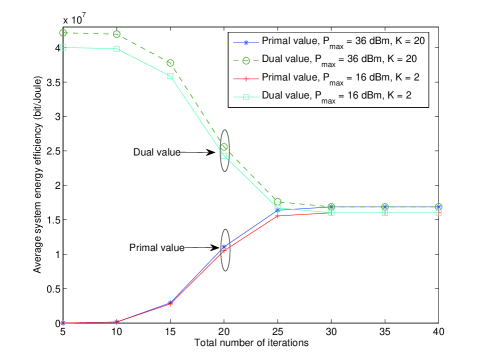
Figure 2: Average system energy efficiency (bit-per-Joule) versus number of iterations with different numbers of users, $K$, and different values of maximum transmit power allowance, $P_{\max}$.

V Simulation Results

In this section, we evaluate the performance of the proposed resource allocation algorithm using simulations. An indoor communication system with a maximum service distance of 10 meters is considered. The TGn path loss model [14] is adopted with a reference distance of $d_{0}=2$ meters. The $K$ users are uniformly distributed between the reference distance and the maximum service distance. The effective antenna gain for each transceiver is assumed to be $14$ dB. The system bandwidth is ${\cal B}=5$ MHz, the number of subcarriers is $n_{F}=128$, and $w_{k}=1,\,\forall k$. Note that by setting $w_{k}=1,\,\forall k$, we obtain the maximum achievable system energy efficiency. We assume a carrier center frequency of $470$ MHz which will be used by IEEE 802.11 for the next generation of Wi-Fi systems [15]. Each subcarrier for RF transmission has a bandwidth of $W=39$ kHz and the noise variance is $\sigma_{z}^{2}=-118$ dBm. The multipath fading coefficients of the transmitter–user links are generated as independent and identically distributed (i.i.d.) Rayleigh random variables with unit variance. The shadowing of all communication links is set to $0$ dB, i.e., $g_{k}=1,\,\forall k$. We assume a static circuit power consumption of $P_{C}=$ 40 dBm, a maximum power grid supply of $P_{PG}=50$ dBm, and a minimum data rate requirement of $R_{\min}=10$ Mbits/s. The minimum required power transfer and the energy harvesting efficiency are set to $P_{\min_{k}}^{req}=-10$ dBm,  $\forall k$, and $\eta_{k}=0.8,\,\forall k,$ respectively. Besides, we assume a power efficiency of $40\%$ for the power amplifier used at the transmitter, i.e., $\varepsilon=\frac{1}{0.4}=2.5$. The average energy efficiency is computed according to (6) and averaged over multipath fading and path loss. In the sequel, the total number of iterations is defined as the number of main loops in Algorithm 1 multiplied with the number of iterations in solving the Layer 1 and Layer 2 problems. Moreover, the step sizes adopted in (19)–(23) are optimized for obtaining a fast convergence. Note that if the transmitter is unable to fulfill the minimum required system data rate $R_{\min}$ or the minimum required power transfer $P^{req}_{\min_{k}}$, we set the energy efficiency and the system capacity for that channel realization to zero to account for the corresponding failure.

V-A Convergence of Iterative Algorithm 1

Figure 2 illustrates the convergence behavior and the duality gap of the proposed iterative algorithm for maximizing the system energy efficiency. The duality gap is defined as the difference between primal optimum and dual optimum (achieved by the proposed algorithm) and indicates the suboptimality due to the constraint relaxation in C6 and insufficient numbers of iterations. We investigate the system performance for different numbers of users, $K$, and different values for the maximum transmit power allowance, $P_{\max}$. The results in Figure 2 were averaged over $10^{5}$ independent channel realizations for both path loss and multipath fading. It can be observed that the energy efficiency of the proposed algorithm converges to the optimum value within 30 iterations for all considered scenarios. The fast convergence and the zero duality gap confirm the practicality of the proposed algorithm.

In the following results, we set the total number of iterations to 30 to illustrate the performance of the proposed algorithm.

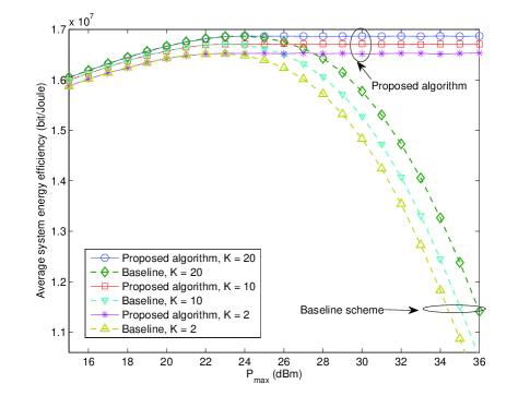
Figure 3: Average system energy efficiency (bit-per-Joule) versus maximum transmit power allowance, $P_{\max}$, for different numbers of users, $K$.

V-B Average Energy Efficiency and Average System Capacity

Figure 3 depicts the average system energy efficiency versus the maximum transmit power allowance, $P_{\max}$, for different numbers of users, $K$. It can be observed that the energy efficiency of the proposed algorithm increases w.r.t. $P_{\max}$ monotonically and reaches an upper limit where the energy efficiency gain due to a higher value of $P_{\max}$ vanishes. This result indicates that once the maximum energy efficiency is achieved by transmitting a sufficiently large power in the RF, any additional increase in the transmitted power will incur a loss in energy efficiency. On the other hand, the energy efficiency of the system increases with the number of users and there are two reasons for this behaviour. First, as the number of users in the system increases, the transmitter has a higher chance to select a user who has a strong channel due to multiuser diversity (MUD). Indeed, the MUD introduces an extra power gain to the system which helps save energy. Second, more idle users harvest the power radiated by the transmitter which reduces the total power consumption of the system, cf. (4). For comparison, Figure 3 also contains the energy efficiency of a baseline scheme which adopts a resource allocation algorithm maximizing the system capacity (bit/s) under constraints C1–C7. It can be seen that in the low transmit power allowance regime, the proposed algorithm performs virtually the same as the baseline scheme. Indeed, the small power radiated by the transmitter creates a bottleneck in the system and the performance of the proposed algorithm is restricted by the limited system resources. However, in the high transmit power allowance regime, the energy efficiency of the baseline scheme decreases dramatically since an exceedingly large transmit power is used for capacity maximization.

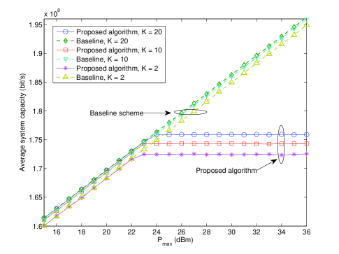
Figure 4: Average system capacity (bit-per-second) versus maximum transmit power allowance, $P_{\max}$, for different numbers of users, $K$.

Figure 4 shows the average system capacity versus maximum transmit power allowance, $P_{\max}$, for different numbers of users, $K$. The proposed algorithm is compared with the baseline scheme described in the last section. It can be observed that both schemes benefit from an increasing number of users due to MUD. On the other hand, the proposed algorithm achieves virtually the same system capacity as the baseline scheme in the low transmit power regime. This suggests that the proposed algorithm transmits with full power in the low transmit power allowance regime. However, as the transmit power allowance increases, the baseline scheme outperforms the proposed algorithm, since the former scheme uses all the available power for capacity maximization which impairs the system energy efficiency.

V-C Average Harvested Power

Figure 5 shows the total average power harvested by the idle users versus the maximum transmit power allowance, $P_{\max}$, for different numbers of users, $K$. It can be observed in Figure 5 that the total average harvested power increases with $P_{\max}$ since more power is available in the RF. On the other hand, a larger portion of the radiated power can be harvested when there are more users in the system since more idle users are participating in the energy harvesting process.

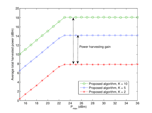
Figure 5: Average total harvested power versus maximum transmit power allowance, $P_{\max}$, for different numbers of users, $K$. The double-sided arrows indicate the power harvesting gain due to an increasing number of users.

VI Conclusions

In this paper, we formulated the resource allocation algorithm design for multiuser OFDM systems as a non-convex and combinatorial optimization problem, in which concurrent wireless information and power transfer were considered. By exploiting nonlinear fractional programming and Lagrange dual decomposition, a novel iterative resource allocation algorithm was proposed for maximizing the system energy efficiency. Simulation results showed that the proposed algorithm converges within a small number of iterations and unveiled the potential benefits of having multiple users for energy efficiency, system capacity, and wireless power transfer.

References

- [1] T. Chen, Y. Yang, H. Zhang, H. Kim, and K. Horneman, “Network Energy Saving Technologies for Green Wireless Access Networks,” IEEE Wireless Commun., vol. 18, pp. 30–38, Oct. 2011.
- [2] O. Arnold, F. Richter, G. Fettweis, and O. Blume, “Power Consumption Modeling of Different Base Station Types in Heterogeneous Cellular Networks,” in Proc. Future Netw. and Mobile Summit, Jun. 2010, pp. 1–8.
- [3] D. W. K. Ng, E. Lo, and R. Schober, “Energy-Efficient Resource Allocation in OFDMA Systems with Large Numbers of Base Station Antennas,” IEEE Trans. Wireless Commun., vol. 11, pp. 3292 –3304, Sep. 2012.
- [4] F. Zhang, S. Hackworth, X. Liu, H. Chen, R. Sclabassi, and M. Sun, “Wireless Energy Transfer Platform for Medical Sensors and Implantable Devices,” in Annual Intern. Conf. of the IEEE Eng. in Med. and Biol. Soc., Sep. 2009, pp. 1045–1048.
- [5] V. Chawla and D. S. Ha, “An Overview of Passive RFID,” IEEE Commun. Magazine, vol. 45, pp. 11–17, Sep. 2007.
- [6] L. Varshney, “Transporting Information and Energy Simultaneously,” in Proc. IEEE Intern. Sympos. on Inf. Theory, Jul. 2008, pp. 1612 –1616.
- [7] P. Grover and A. Sahai, “Shannon Meets Tesla: Wireless Information and Power Transfer,” in Proc. IEEE Intern. Sympos. on Inf. Theory, Jun. 2010, pp. 2363 –2367.
- [8] R. Zhang and C. K. Ho, “MIMO Broadcasting for Simultaneous Wireless Information and Power Transfer,” in Proc. IEEE Global Telecommun. Conf., Dec. 2011, pp. 1 –5.
- [9] Z. Xiang and M. Tao, “Robust Beamforming for Wireless Information and Power Transmission,” IEEE Commun. Lett., vol. 1, pp. 372 –375, Aug. 2012.
- [10] W. Dinkelbach, “On Nonlinear Fractional Programming,” Management Science, vol. 13, pp. 492–498, Mar. 1967. [Online]. Available: http://www.jstor.org/stable/2627691
- [11] C. Y. Wong, R. S. Cheng, K. B. Letaief, and R. D. Murch, “Multiuser OFDM with Adaptive Subcarrier, Bit, and Power Allocation,” IEEE J. Select. Areas Commun., vol. 17, pp. 1747–1758, Oct. 1999.
- [12] D. W. K. Ng, E. S. Lo, and R. Schober, “Energy-Efficient Resource Allocation in Multi-Cell OFDMA Systems with Limited Backhaul Capacity,” IEEE Trans. Wireless Commun., vol. 11, pp. 3618–3631, Oct. 2012.
- [13] S. Boyd and L. Vandenberghe, Convex Optimization. Cambridge University Press, 2004.
- [14] IEEE P802.11 Wireless LANs, “TGn Channel Models”, IEEE 802.11-03/940r4, Tech. Rep., May 2004.
- [15] H.-S. Chen and W. Gao, “MAC and PHY Proposal for 802.11af,” Tech. Rep., Feb., [Online] https://mentor.ieee.org/802.11/dcn/10/11-10-0258-00-00af-mac-and-phy-proposal-for-802-11af.pdf.