Incommensurability Effects in Odd Length $J_{1}$-$J_{2}$ Quantum Spin Chains:
On-site magnetization and Entanglement

Abstract

For the antiferromagnetic $J_{1}$-$J_{2}$ quantum spin chain with an even number of sites, the point $J_{2}^{d}=J_{1}/2$ is a disorder point. It marks the onset of incommensurate real space correlations for $J_{2}>J_{2}^{d}$. At a distinct larger value of $J_{2}^{L}=0.52036(6)J_{1}$, the Lifshitz point, the peak in the static structure factor begins to move away from $k=\pi$. Here, we focus on chains with an odd number of sites. In this case the disorder point is also at $J_{2}^{d}=J_{1}/2$ but the behavior close to the Lifshitz point, $J_{2}^{L}\simeq 0.538J_{1}$, is quite different: starting at $J_{2}^{L}$, the ground state goes through a sequence of level crossings as its momentum changes away from $k=\pi/2$. An even length chain, on the other hand, is gapped for any $J_{2}>0.24J_{1}$ and has the ground state momentum $k=0$. This gradual change in the ground state wave function for chains with an odd number of sites is reflected in a dramatic manner directly in the ground state on-site magnetization as well as in the bi-partite von Neumann entanglement entropy. Our results are based on DMRG calculations and variational calculations performed in a restricted Hilbert space defined in the valence bond picture. In the vicinity of the point $J_{2}=J_{1}/2$, we expect the variational results to be very precise.

I Introduction

Disorder points were first discussed by Stephenson in models described by classical statistical mechanics. Stephenson (1969, 1970a); Stephenson and Betts (1970); Stephenson (1970b) On one site of a disorder point, the correlation function shows monotonic decay, on the other oscillatory decay. Depending on the how the wavelength of the oscillation depends on the temperature, one distinguishes between two kinds of disorder points. If the wavelength of the oscillation depends on the temperature, one speaks of a disorder point of the first kind, if it does not, one speaks of a disorder point of the second kind. Stephenson (1970a) In the first studies, disorder points were found where the paramagnetic phase of frustrated two-dimensional Ising models starts to show incommensurate instead of commensurate behavior. In models with competing commensurate and incommensurate order one might expect such a point to occur where the short-range correlations with the largest correlation length change from being commensurate to being incommensurate. Such a point should then be associated with a cusp in the correlation length, a fact that was quickly established. Stephenson (1970c) Schollwöck, Jolicoeur and Garel first investigated disorder points in a quantum spin chain for the bilinear-biquadratic $S=1$ quantum spin chain, Schollwöck et al. (1996) which has $H=\cos{\theta}\sum\mathbf{S_{i}}\cdot\mathbf{S_{i+1}}+\sin{\theta}\sum\mathbf{S_{i}}\cdot\mathbf{S_{i+1}}$. They pointed out that the disorder point in this gapped quantum model coincides with the AKLT-point where $\tan{\theta_{VBS}}=1/3$ and the known ground state is a valence bond solid (VBS) with correlation length $\xi=1/\ln(3)$. They also identified another distinct point, the Lifshitz point, at $\tan{\theta_{L}}=1/2$, where the peak in the structure factor is displaced away from $\pi$ due to incommensurability effects. A third distinct point in this $S=1$ model, $\tan{\theta_{disp}}\simeq 0.4$, has also been located Golinelli et al. (1999) where the minimum in the magnon dispersion shifts away from $\pi$ and the curvature (velocity) vanishes. These 3 points can be distinct since no phase transition occurs and the correlation length remains finite. Subsequently it was confirmed Bursill et al. (1995) that for the $S=1/2$ $J_{1}$-$J_{2}$ spin chain with Hamiltonian:

$$H=J_{1}\sum_{i}\mathbf{S}_{i}\cdot\mathbf{S}_{i+1}+J_{2}\sum_{i}\mathbf{S}_{i}\cdot\mathbf{S}_{i+2},\ J_{1},J_{2}>0\ ,$$ (1)

the situation is similar. For the calculations presented in this paper, we set $J_{1}\equiv 1$ and vary the remaining parameter $J_{2}$. The disorder point, with minimal correlation length ($\xi\simeq 0$), occurs at the Majumdar-Ghosh Majumdar (1970) (MG) point, $J_{2}^{d}=J_{1}/2$, and the Lifshitz point at $J_{2}^{L}=0.52036(6)J_{1}$. Bursill et al. (1995)

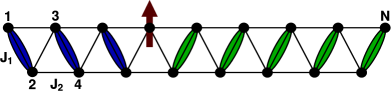
Figure 1: (Color online.) The odd length $J_{1}$-$J_{2}$ chain. Two different dimerization patterns are separated by a soliton.

At the disorder points, the ground states of these two quantum spin models share important features: the system is gapped and an exact wave function is known. For both, the momentum of the lowest excitations changes at a distinct point. Yet, there are also important differences between the two systems. While the $S=1$ VBS state remains an exact state for a chain with an odd number of spins, this is not the case for the $S=1/2$ $J_{1}$-$J_{2}$ chain at the MG point where no analytical expression for the odd length ground state wave function is known. Moreover, the odd length $J_{1}$-$J_{2}$ chain is gapless in the thermodynamic limit within the $S_{Tot}=1/2$ subspace, and a large spin gap exists. The onset of incommensurability effects for odd length chains must then be quite distinct from the onset in even length chains. Here, we show that this is indeed the cases. While the disorder point remains unchanged, the nature of the Lifshitz point, $J_{2}^{L}\simeq 0.538J_{1}$, is rather different. At $J_{2}^{L}$, a sequence of level crossings starts, changing the ground state momentum away from $k=\pi/2$. Although the correlation length remains small, the change in ground state momentum induces pronounced oscillations directly in the on-site magnetization as well as the entanglement entropy. The modulations in the on-site magnetization are potentially observable in experiments. This scenario is reminiscent of a real Lifshitz transition Lifshitz (1960); Hornreich et al. (1975); Blanter et al. (1994); Yamaji et al. (2006) in which the ground state becomes modulated. The scaling of the entanglement entropy at Lifshitz transitions recently has been the subject of interest. Fradkin (2009); Rodney et al. (2012)

The $S=1/2$ $J_{1}$-$J_{2}$ antiferromagnetic (AF) spin chain is one of the simplest frustrated Heisenberg spin models, but it has a rich phase diagram. The system undergoes a transition Haldane (1982) from a gapless Luttinger liquid to a dimerized phase at a critical value of $J^{c}_{2}=0.241167J_{1}$. Tonegawa and Harada (1987); Okamoto and Nomura (1992); Eggert (1996) For even length chains the ground state wave function at the MG point $J_{2}=J_{1}/2$ is known to be formed by nearest neighbor dimers. Majumdar and Ghosh (1969); Majumdar (1970); Broek (1980) It is two-fold degenerate, corresponding to the two possible nearest neighbor dimerization patterns, indicated in Fig. 1. As is evident from Fig. 1, an unpaired spin, a soliton, Shastry and Sutherland (1981); Caspers et al. (1984) can act as a ’domain wall’ and separate regions of different dimerization patterns. In the Luttinger liquid phase unpaired spins are more commonly called spinons since they do not act as domain walls. Spin excitations in the even length chain correspond to introducing two solitons and it is known Sørensen et al. (1998) that in the vicinity of the MG point the solitons do not bind and a large spin gap of $\Delta=2\Delta_{sol}$ (at the MG point $\Delta_{sol}/J_{1}=0.1170(2)$) Sørensen et al. (1998) exists. The spin gap for even length chains is known to remain sizable Chitra et al. (1995); White and Affleck (1996) beyond $J_{2}^{L}$. The presence of a large soliton mass, $\Delta_{sol}$, renders variational calculations based on a reduced Hilbert space consisting of soliton states very precise; Shastry and Sutherland (1981); Caspers et al. (1984) a fact that we shall exploit here.

In contrast, for odd length chains it is not possible for the chain to be fully dimerized and the ground state wave function is not known for any value of $J_{2}$. An $S=1/2$ soliton that effectively behaves as a free particle Uhrig et al. (1999a) is always present in the ground state and gives rise to gapless excitations. Depending on the quantity in question, odd and even length chains can show very different behavior. Under open boundary conditions (OBC), this has for example already been seen in the on-site magnetization, Sørensen et al. (1998) the entanglement entropy Sørensen et al. (2007); Affleck et al. (2009) and the negativity. Deschner and Sørensen (2011) As mentioned, here we focus on odd length chains.

While it is possible to perform highly precise density matrix renormalization group (DMRG) calculations well beyond the onset of incommensurability for even chains, White and Affleck (1996); Chitra et al. (1995) the sequence of level crossings that we encounter for odd length chains for $J_{2}>J_{2}^{L}$ significantly restrains the usefulness of the DMRG technique in a large region of parameter space for $J_{2}>J_{2}^{L}$. Fortunately, using the picture of Shastry and Sutherland, Shastry and Sutherland (1981) it is possible to quite efficiently perform very precise variational calculations for both open and periodic boundary conditions (PBC). Here, we mainly present results of such variational calculations and supplement them with DMRG-results.

A number of spin-Peierls compounds, which to some extent realize the $J_{1}$-$J_{2}$ spin chain, have been identified. One of the most well known is CuGeO₃. Hase et al. (1993) In these materials impurities often cut the chains at random points. Therefore both odd and even length chains are present. A particular point of focus has been the study of $S=1/2$ solitons Fagot-Revurat et al. (1996, 1997); Horvatić et al. (1999); Uhrig et al. (1999b) in these systems. Thus, our results might be directly verifiable if materials with sufficiently large $J_{2}>J_{2}^{d}$ can be found.

The outline of the paper is as follows. In section II the variational approach is described. Section III begins with a presentation of our DMRG results for the correlation functions, correlation lengths and the structure factor. In section III.1 we discuss our variational results for the $J_{1}$-$J_{2}$ with periodic boundary conditions and show the change in ground state momentum developing at the Lifshitz point. Section III.2 contains variational and DMRG results for the on-site magnetization and level crossings occurring with open boundary conditions. Variational and DMRG results for the entanglement entropy for a range of $J_{2}$ for odd length chains (OBC) are presented in section IV and contrasted with results for even length chains (OBC). Finally, estimates for the location of the Lifshitz point are presented in section V.

In the following, we shall take $J_{1}\equiv 1$. This leaves us with only one parameter, $J_{2}$, that governs the properties of the system.

II The variational method

Most of the results presented in this paper were generated using variational calculations, Shastry and Sutherland (1981); Caspers et al. (1984); Zeng and Parkinson (1995); Sørensen et al. (2007); Deschner and Sørensen (2011) i.e. the results were obtained by minimizing the expectation value of the Hamiltonian within a reduced Hilbert-space:

$$\langle H\rangle=\frac{(\varphi|H\varphi)}{(\varphi|\varphi)}\ ,$$ (2)

where

$$\varphi=\sum c_{j}\varphi_{j}$$ (3)

and the minimization is done with respect to the $c_{j}$. To get a good estimate of the true ground state of the system, it is necessary that the ground state has a sizable projection onto the subspace one diagonalizes in. The quality of the result of a variational calculation thus depends very strongly on the choice of subspace. Often one has to rely on physical insight and intuition to choose well. For the $J_{1}$-$J_{2}$-model, which we consider, the selection of an appropriate subspace is straight-forward as long as one stays in the dimerized phase. In contrast, in the Luttinger liquid phase, selecting an appropriate subspace seems intractable.

The first variational calculations on the $J_{1}$-$J_{2}$-model were done in a space that we in the following shall call $R_{0}$. Shastry and Sutherland (1981); Caspers et al. (1984) It is spanned by the states in which there are domains that have one of the two ground state configurations of the MG-chain and which are separated by one soliton. Examples can be seen in Figs. 1 and 2. The arrows in Fig. 2 serve to fix the phase of the dimers that make up the ground state. Our convention is such that if the arrow goes from site $i$ to site $j$ the spins are in the state: $\frac{1}{\sqrt{2}}(|\uparrow\rangle_{i}|\downarrow\rangle_{j}-|\downarrow\rangle_{i}|\uparrow\rangle_{j})$.

(a)

(b)

Figure 2: Two variational states used in the calculations within $R_{0}$ for a chain with an odd number of sites. The arrows between sites are used to fix the phase of the dimers (see main text).

For a chain with an odd number of sites, a set of single soliton states can be generated by leaving the chain maximally dimerized and taking the remaining site to be in the $S_{z}$$=$$1/2$-state. For a chain with open boundary-conditions, the soliton can only reside on every second site. The dimension of this variational subspace is then $D$$=$$(N+1)/2$. We use $N$ to denote the length of the chain. For calculations on odd length chains with periodic boundary conditions it is necessary to allow a nearest neighbor dimer across the boundary and to let the soliton cross the boundary by going from site $N$ to site 2. In this case $R_{0}$ has dimension $N$ and incorporates states with the soliton at every site with the remaining spins paired in nearest neighbor dimers. (For odd $N$ and PBC it becomes difficult to distinguish the 2 dimerization patterns since they twist into each other at the boundary. Still, the soliton clearly denotes a ’domain wall’ between the two patterns).

To improve upon $R_{0}$, it is natural to act with the Hamiltonian onto the space as doing this repeatedly generates a space that contains the ground state if the starting space had any overlap with and all symmetries of the ground state. It was shown that acting onto $R_{0}$ with the Hamiltonian only once is at the MG point already enough to make the calculation almost exact.Caspers et al. (1984) For the $J_{1}$-$J_{2}$-model with $J_{2}\neq 0.5J_{1}$ the linearly independent states generated by acting with the Hamiltonian onto $R_{0}$ fall into three classes, each of which corresponds to a variational subspace:

• The variational space $R_{0}$: Spanned by the states that are in $R_{0}$.

• The variational space $R_{1}$: Spanned by states in which sites to the left and right of the soliton are connected by a valence bond. Pictorial representations of example-states are shown in Fig. 3.

• The variational space $R_{2}$: Spanned by states in which two neighboring sites are in a valence bond with their next-nearest neighbor. These states are generated by the action of the nearest-neighbor-terms and the next-nearest neighbor terms in the Hamiltonian on adjacent dimers in the states in $R_{0}$. Pictorial representations of example-states are shown in Fig. 4. In the case of the MG-chain, $J_{1}$ and $J_{2}$ are balanced in such a way that these states are not generated because they occur with a weight of $2J_{2}-J_{1}$.

The number of states in $R_{0}$ and $R_{1}$ scales linearly with the size of the chain, whereas the number of states in $R_{2}$ scales quadratically. Due to computational cost we have thus not found it practical to use the union of the three as the variational subspace for chains longer than 101 sites. We performed calculations using the union of $R_{0}$ and $R_{1}$ (in the following called $Z_{s}$) for chains up to $1001$ and the union of all three (in the following called $Z_{b}$) for a chain of $101$ sites. In this way we could go to long chains and also check the validity through the comparison at $N=101$. We found that while there were small quantitative differences between calculations done in $Z_{s}$ and $Z_{b}$ the overall qualitative features of the results where the same. Therefore, we chose to use $Z_{s}$, the union of $R_{0}$ and $R_{1}$, or just $R_{0}$ for the variational calculations shown in this paper.

All the states in these spaces have $S_{z}^{Tot}:=\sum_{i}S_{z}^{i}=1/2$. We could equally well have worked in the $S_{z}^{Tot}=-1/2$ space. States of higher total spin are of little importance to the low-energy physics since they contain more solitons and are thus gapped by at least twice the soliton mass $\Delta_{sol}$. Since $\Delta_{sol}$ is sizable Sørensen et al. (1998) in the regime of our study, such states can be disregarded for both odd and even $N$.

(a)

(b)

Figure 3: Two variational states used in the calculations within $R_{1}$ for a chain with an odd number of sites. The arrows between sites are used to fix the phase of the dimers (see main text).

(a)

(b)

(c)

Figure 4: Three states that are generated by acting with the Hamiltonian onto $R_{0}$. The arrows between sites are used to fix the phase of the dimers (see main text).

A variational description of a chain with an even number of sites can be done along the same lines. Again, the states are chosen in order to leave all but two spins in the favored dimerized state. In this way one can gain insight into the low-energy singlet- as well as triplet-excitations by choosing the two spins to be in singlet- or the triplet-states respectively.

If one considers a subspace with an orthogonal basis, one can just diagonalize the Hamiltonian. While an easy way to orthogonalize $R_{0}$ is known, Uhrig et al. (1999a) this is generally not true for other subspaces. Importantly, for $R_{1}$ no such method is known. We thus have to solve the generalized eigenvalue-problem given by

$$\mathfrak{H}\;\vec{\varphi}=\lambda\;\mathfrak{B}\vec{\varphi}\ ,$$ (4)

where $\mathfrak{H}_{ij}:=(\varphi_{i}|H\varphi_{j})$ and $\mathfrak{B}_{ij}:=(\varphi_{i}|\varphi_{j})$. Such generalized-eigenvalue-problems can be solved numerically by standard routines. We calculate $\mathfrak{H}$ and $\mathfrak{B}$ by evaluating their defining expressions. This is possible because for valence-bond-states the action of $H$ on them as well as the overlap between them can straightforwardly be calculated in an automated manner. How to do all other calculations necessary to get the results presented in this paper has already been described in an earlier publication. Deschner and Sørensen (2011) We took the coefficients $c_{j}$ in Eq. (3) to be real. Also for PBC, the resulting wave function is not an eigenstate of the translational operator which would have required the use of complex $c_{j}$’s. Effectively we obtain states that are linear combinations of translationally invariant states with $k$ and $-k$, degenerate in energy. While this has no bearing on the obtained energies, it affects real-space quantities like the on-site magnetization and entanglement which cannot be translational invariant.

III The incommensurate behavior

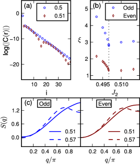
Figure 5: (Color online.) (a) The spin-spin correlation function $C(r)=\langle S_{i}S_{i+r}\rangle$ for a chain with 201 sites and $J_{2}=0.5,0.51$. The correlation-length (b) and the static structure factor (c) for chains with an odd (201) or an even (200) number of sites. The data was obtained with DMRG. Open boundary conditions were employed and $m=256$ states kept. For both, odd and even length chains, the correlation-length displays a minimum at the MG point. The static structure factors of odd and even are shown for $J_{2}=0.51$ and $J_{2}=0.57$. The maximum remains at $q=\pi$ until the Lifshitz point is crossed (not shown in figure).

Previous numerical studies of disorder points in $S=1/2$ Tonegawa and Harada (1987); Nomura and Okamoto (1993, 1994); Bursill et al. (1995); Chitra et al. (1995); White and Affleck (1996) and $S=1$ Schollwöck et al. (1996); Kolezhuk et al. (1996); Roth and Schollwöck (1998); Polizzi et al. (1998); Golinelli et al. (1999) quantum spin chains have concentrated on the behavior of even length chains. For the $S=1/2$ $J_{1}$-$J_{2}$ chain it has been shown that the disorder point of this $1$-dimensional quantum system can be understood as a $1+1$ dimensional classical disorder point. In particular, it was shown Garel and Maillard (1986); Fáth and Sütő (2000); Nomura (2003) that in the “commensurate” region of the phase diagram the correlation function behaves asymptotically, with $r\gg\xi$, as

$$\langle S_{i}S_{i+r}\rangle\sim(-1)^{r}\frac{e^{-r/\xi}}{\sqrt{r}},$$ (5)

and in the “incommensurate” region of the phase diagram as

$$\langle S_{i}S_{i+r}\rangle\sim(-1)^{r}\frac{e^{-r/\xi}}{\sqrt{r}}\cos\left[(q-\pi)r+\phi\right].$$ (6)

Here, $q$ is the wave vector of the incommensurate correlations and $\phi$ a phase shift. However, right at the disorder point separating commensurate and incommensurate correlations the correlation function is asymptotically purely exponential:

$$\langle S_{i}S_{i+r}\rangle\sim(-1)^{r}e^{-r/\xi}.$$ (7)

For these quantum spin models it appears that this purely exponential behavior is in part connected to the fact that the ground state is an exact nearest neighbor dimer state. Interestingly, as we shall see, the correlation functions at the MG point for odd length chains display the same behavior in the absence of a unique nearest neighbor dimer ground state. Furthermore, it is known Garel and Maillard (1986); Fáth and Sütő (2000) that as the disorder point is approached from the commensurate side, the derivative of the correlation length with respect to the driving coupling becomes infinite, while it is finite on the incommensurate side. It is also known that the disorder point has special degeneracies that are exact for any system size $N$. For instance, for the $J_{1}$-$J_{2}$ chain with periodic boundary conditions and an even length, the two dimerization patterns are degenerate at the disorder point while their symmetric and antisymmetric combinations are split with an exponentially small gap away from this point.

We now present our results for the incommensurate effects in odd length $S=1/2$ $J_{1}$-$J_{2}$ chains. Our first point of focus is the location of the disorder point. As stressed above, when $N$ is odd, the nearest neighbor dimer wave function is not an exact solution Shastry and Sutherland (1981) and there are also no special degeneracies. There is therefore no reason to expect that the behavior of the correlation length at the MG point is in any way unique. However, as we shall see, this is indeed the case. DMRG results for $C(r)=\langle S_{i}S_{i+r}\rangle$ for an open chain with $N=201$ are shown in Fig. 5(a) for $J_{2}=0.5$ and $0.51$. The correlation function follows a purely exponential decay at the MG point, $J_{2}=0.5$, with a finite correlation length:

$$\xi_{\mathrm{MG}}\sim 2.8\ \ (\mathrm{odd}\ N).$$ (8)

Distant spins in odd chains are correlated even at the MG point, because the soliton is present in the chain. The correlations can be thought of as correlations in the soliton wave function. Secondly, as can be seen in Fig. 5(a), incommensurate correlations are clearly present for $J_{2}=0.51$. They were present in every calculation we performed with $J_{2}>0.5$. We conclude that the disorder point remains at $J_{2}=J_{1}/2$ albeit with a finite correlation length compared to the case of even $N$ where the correlation length is nominally zero.

The precise behavior of the correlation length around the disorder point $J_{2}=1/2$ appears to have been studied neither for even length nor for odd length chains. Results for larger $J_{2}>0.6$ are available for even $N$. White and Affleck (1996) By fitting DMRG results for chains of $200$ and $201$ sites to the forms Eqs. (5), and (6) we have determined $\xi$ as a function of $J_{2}$ for both even and odd $N$ (see Fig. 5(b)). The results for the even and the odd length chain are remarkably similar. At the disorder point there is a discontinuity in the slope of $\xi$ and on the commensurate side the slope of $\xi$ approaches $-\infty$. We found that close to the disorder point in the commensurate region combined forms like $|C(r)|\sim C\exp(-r/\xi_{C})/\sqrt{r}+D\exp(-r/\xi_{D})$ with $\xi_{C}>\xi_{D}$ fit the data better than the single forms Eq. (5), and (6), because the dominant short-ranged correlations change at the disorder point. The results presented in Fig. 5 do not use such combined forms. We also note that for odd $N$ and for a range of $J_{2}>0.538$ it becomes very difficult to obtain reliable DMRG results due to the appearance of many almost degenerate states.

The structure factor for even chains has been studied in some detail previously, Tonegawa and Harada (1987); Bursill et al. (1995) and the Lifshitz point has been located, $J_{2}^{L}=0.52036(6)$. Bursill et al. (1995) Our DMRG results are shown in Fig. 5(c). In agreement with previous studies for even $N$, we observe that the maximum in the structure factor remains at $q=\pi$ for $J_{2}=0.51$ but has clearly moved away from $\pi$ at $J_{2}=0.57$. This is clearly also the case for odd $N$. Due to the above mentioned difficulties in obtaining reliable DMRG results for odd $N$ and $J_{2}>0.538$ we have not been able to determine the precise point where the peak in the structure factor is displaced from $q=\pi$. Using the variational techniques outlined above it is possible to understand in detail what happens close to $J_{2}\simeq 0.538$.

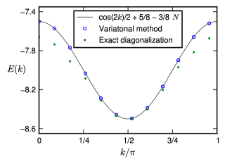
Figure 6: (Color online.) Comparison of the estimate by Shastry and Sutherland Shastry and Sutherland (1981), the variational method and exact diagonalization (ED) data. Sørensen et al. (1998) Data was taken for a chain with 23 sites and $J_{2}$=$0.5$. Only the lowest energy of a spin $1/2$ excitation for every momentum is shown. The deviations to ED occur at higher energies where the dispersive mode enters the continuum and the variational calculation is only of limited value.

III.1 Variational Results in Periodic Boundary Conditions

We now turn to a discussion of our variational results obtained using the method outlined in section II. We begin by focusing on the case of odd length chains and periodic boundary conditions. The case of open boundary conditions will be the subject of the next subsection. The results shown in this subsection were obtained using the space $R_{0}$ (see section II), consisting of all single soliton states with $S_{z}^{Tot}=1/2$.

At the MG point the spectrum of the $J_{1}$-$J_{2}$-model has been studied extensively. The feature that is most important to us is the low-lying dispersive line that is well separated from the continuumSørensen et al. (1998) and roughly follows a cosine as found in previous variational studies. Shastry and Sutherland (1981); Arovas and Girvin (1992)

$$E(k)=\frac{1}{8}\left(5+4\cos(2k)-3N\right).$$ (9)

Our variational method reproduces this estimate and agrees well with the low-energy data of an exact diagonalization of a chain of 23 sites (see Fig. 6). It may be surprising that the minimum of the dispersion relation is not at $k=\pi$ but at $k=\pi/2$. This is a natural consequence of the effective doubling of the unit cell that occurs because the action of the Hamiltonian displaces the soliton by two sites.

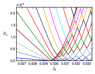
Figure 7: (Color online.) The excitation spectrum with periodic boundary conditions in the variational subspace with $S_{z}^{Tot}=1/2$. The energies of the first few excited states are shown. The ground state energy was set to zero. The energies of the excited states approaches the ground state energy until, at $J_{2}=J_{2}^{L}$, level-crossings start to occur. All energy-levels are doubly degenerate. The data was taken for a chain with 401 sites.

One of the strengths of the variational method is that within the limits of the approximation it is possible to easily access not only the ground state but also the entire energy spectrum within the variational subspace of $S_{z}^{Tot}=1/2$ states. Computing the spectrum through the transition region reveals very surprising behavior (see Fig. 7). All the states are two-fold degenerate corresponding to the energetically degenerate $k$ and $-k$. As one approaches the transition, the excited states linearly move closer and closer to the ground state. At the Lifshitz point $J_{2}^{L}\approx 0.53$ the energy of the first excited state crosses the ground state energy. This level crossing marks the first shift in the ground state momentum and is followed by a series of other level crossings at larger $J_{2}$ that further shift the ground state momentum. Clearly, the presence of the many adjacent level crossings hinders the effectiveness of DMRG calculations.

This is in stark contrast to the spectrum of even length chains: The ground state of even length chains is exactly two fold degenerate at the MG point for any $N$ whereas for larger $J_{2}$ the symmetric and antisymmetric combinations are split with an exponentially small gap in $N$. The excited states are separated from these two states by a large gap of approximately $2\Delta_{sol}$. This gap persists throughout the transition region and no level crossings are observed. Tonegawa and Harada (1987); White and Affleck (1996)

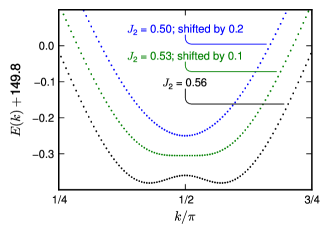
Figure 8: (Color online.) Dispersion relation for varying $J_{2}$. The data was taken for a chain with 401 sites. To avoid cluttering, the dispersion relations for the smaller two $J_{2}$ were shifted. As $J_{2}$ is increased, the minimum first flattens and then turns into a local maximum.

It is very instructive to look at how the dispersion relation in Fig. 6 evolves with $J_{2}$. As can be seen in Fig. 8, the dispersion relation changes its shape when $J_{2}$ is increased. The minimum at $k=\pi/2$ first becomes flat very close to $J_{2}=0.53$ and then becomes a local maximum. In the process two minima are created, which move away from $k=\pi/2$ with increasing $J_{2}$. The ground state momentum is then clearly changing away from $k=\pi/2$ beyond $J_{2}=0.53$ and we may identify the point where this happens with a real Lifshitz transition Hornreich et al. (1975); Hornreich and Bruce (1978); Hornreich (1980); Michelson (1977a, b, c) as opposed to the corresponding point in the $S=1$ bilinear biquadratic chain where the ground state momentum remains unchanged and the shift is in the excited magnon dispersion. Due to the shift in the ground state momentum we conclude that the maximum of the structure factor will shift away from $k=\pi$ at the same point. This is consistent with the data in Fig. 5. We therefore in the following refer to this point as the Lifshitz point, $J_{2}^{L}$.

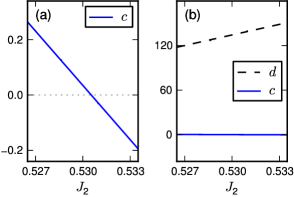
Figure 9: (Color online.) The second-order coefficient of the dispersion relation $c$ changes sign ((a), (b)) while the forth-order coefficient $d$ stays positive (b). The data are results off a fit to data of the kind shown in Fig. 8. The dotted horizontal line in (a) separates positive from negative values.

The precise behavior of the dispersion relation close to $J_{2}^{L}$ is analyzed in Fig. 9.

For a range of $J_{2}$, we fitted the dispersion relation to the form Golinelli et al. (1999)

$$E(k)=E(k_{0})+\frac{c}{2}(k-k_{0})^{2}+\frac{d}{24}(k-k_{0})^{4}$$ (10)

and confirmed that the second-order coefficient $c$ changes its sign at a $J_{2}$ close to 0.53 while the fourth order coefficient $d$ stays positive (see Fig. 9). This behavior is typical of a Lifshitz transition and if the coefficient $c=v^{2}/\Delta_{sol}$ is associated with a velocity, $v$, the Lifshitz point signals the vanishing of this velocity. Golinelli et al. (1999)

The variational calculations with periodic boundary conditions presented in this section were limited to the subspace $R_{0}$ described in section II. This basis only includes nearest neighbor valence bonds and it is quite noteworthy that the physics of the Lifshitz point along with the associated level crossings are captured within this simple basis set. However, as we discuss in section V we do not expect the precise location of the Lifshitz point to be accurately determined within $R_{0}$.

III.2 Open boundary conditions

In materials that realize the $J_{1}$-$J_{2}$ spin chain impurities are always present. They often act as non-magnetic impurities effectively breaking the linear chains into finite segments. The use of open boundary conditions is therefore closer to the experimental situation than the use of periodic boundary conditions. Furthermore, it is natural to expect half of the chain segments to have an odd number of sites. In this subsection we therefore focus on odd length chains with open boundary conditions. In particular, we describe the change that switching from periodic to open boundary conditions causes. The variational results shown in this subsection were obtained using the space $Z_{s}$ (see section II).

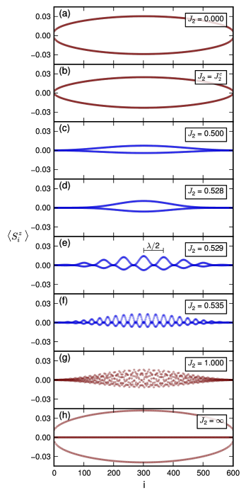
Figure 10: (Color online.) The on-site magnetization at a range of values of $J_{2}$ for $N=601$ sites. Additional structure appears beyond $J_{2}^{L}$. For $J_{2}=0$, $J_{2}^{c}$, $1$ and $\infty$ DMRG-data (obtained with $m=256$ states kept) are shown (red). For the remaining $J_{2}$ variational calculations are shown (blue).

One quantity that very directly shows the qualitative difference between PBC and OBC is the ground state on-site or local magnetization, $\langle S^{z}_{i}\rangle$, which is of importance to for instance NMR measurements. Fagot-Revurat et al. (1996, 1997) Figure 10 shows the on-site magnetization at 8 different values of the frustrating interaction $J_{2}$ between $J_{2}=0$ and $J_{2}=\infty$ in a chain of 601 sites. The figures 10(c)-(f) show variational calculations through the Lifshitz point $J_{2}^{L}$ where DMRG calculations are less effective, the remaining results (a),(b),(g) and (h) are obtained with DMRG.

The Luttinger liquid phase ($J_{2}\leq J_{2}^{c}$): The transition to the dimerized phase occurs at $J_{2}^{c}$, see Fig. 10(b). At this point, as well as throughout the Luttinger liquid phase ($J_{2}<J_{2}^{c}$), the on-site magnetization agrees very well with the prediction for the on-site magnetization in the ground state with $S_{z}^{Tot}=1/2$ from conformal field theory: Eggert et al. (2002)

$$\langle S^{z}_{i}\rangle=C(-1)^{i}\sqrt{\frac{\pi}{2N}\sin\left(\frac{\pi i}{N}\right)}+\frac{1}{2N},$$ (11)

where $C$ is a constant. In this phase $\langle S^{z}_{i}\rangle$ increases with the characteristic behavior $\langle S^{z}_{i}\rangle\sim\sqrt{i}$ for small $i$ close to the boundary.

Dimerized phase with $J_{2}<J_{2}^{L}$: Once the dimerized phase is entered $\langle S^{z}_{i}\rangle$ is drastically altered. The on-site magnetization roughly follows the behavior of a massive particle in a box Sørensen et al. (2007) with $\langle S^{z}_{i}\rangle\sim i^{2}$ close to the boundary. This behavior is clearly visible at the MG point (Fig. 10(c)). As $J_{2}$ is increased beyond the MG point towards the Lifshitz point $J_{2}^{L}$ the central peak sharpens (Fig. 10(d)).

’Incommensurate’ phase $J_{2}>J_{2}^{L}$: At the Lifshitz point there is another dramatic change in $\langle S^{z}_{i}\rangle$: additional maxima develop and the magnetization is modulated by an oscillating function (Fig. 10(e)). Upon increasing $J_{2}$ further, more such maxima form and the wave-length of the modulation decreases (see figures 10(f) and (g)). If $J_{2}$ is fine tuned for a given $N$ it is possible to find a point where 2 maxima occur in $\langle S^{z}_{i}\rangle$, then 3 maxima and so forth.

It is natural to expect this behavior based on the results for PBC presented in section III.1. The local magnetization is effectively modulated with the momentum of the ground state. The running wave found under periodic boundary conditions is converted to a standing wave under open boundary conditions. Then, as the momentum of the ground states changes with growing $J_{2}$, the wave-length of the modulation shrinks. Finally, in Fig. 10(h) we show results for $J_{2}\to\infty$. In this limit the odd length chain with $N$ sites is split into 2 chains with $(N-1)/2$ and $(N+1)/2$ sites one of which will have an even number of sites and hence $\langle S^{z}_{i}\rangle\equiv 0$. The on-site magnetization of the other chain can be found by calculating $\langle S^{z}_{i}\rangle$ for a chain with $J_{2}=0$ of the same length. The results shown in Fig. 10(h) were obtained in this way, i.e. from data for a chain with $N=301$ and $J_{2}=0$ that was then interspersed with zeros from the half of the chain that had an even number of sites.

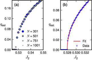
Figure 11: (Color online.) The wave number $q_{\mathrm{est}}$ against $J_{2}$. Data is shown for four chains of different length (a) and with the result of a fit $q_{\mathrm{est}}=1.2062\ \Theta(J_{2}-0.528)(J_{2}-0.528)^{0.4806}$ for a chain of 601 sites (b).

To estimate the wave-length of the incommensurate modulation we make use of the fact that, if our system had translational invariance, the distance between maxima in the on-site magnetization would be equal to half of the wave-length, as indicated in Fig. 10(e). Thus, by calculating the mean distance of the central maxima, we are able to determine an estimate for the wave-length of the incommensurate modulation. The inverse of this quantity can then be used to calculate the wave number, $q_{\mathrm{est}}=2\pi/\lambda_{\mathrm{est}}$. In Fig. 11(a) we show how $q_{\mathrm{est}}$ varies with $J_{2}$ for four chains whose length ranges from 301 to 1001 sites.

Since the incommensurate behavior can only be seen if the wave-length is shorter than the system, it starts later in smaller chains. Aside from small deviations, that can be attributed to finite size effects, the wave-length does only depend on $J_{2}$ and not the length of the chain (see Fig. 11(a)). In the limit of infinite $J_{2}$, the next-neighbor interaction $J_{1}$ can be neglected and the chain be partitioned into two sub-chains that do not interact. As mentioned, the $J_{1}$-$J_{2}$-model in this limit approaches two uncoupled chains with intra chain coupling $J_{2}$. The wave-length of the incommensurate behavior in this limit reaches its minimum with $\lambda=4$ lattice spacings.

For $J_{2}>J_{2}^{\mathrm{L}}$, one expects the wave number $q$ to behave as $q\propto(J_{2}-J_{2}^{\mathrm{L}})^{\alpha}$, where $0<\alpha<1$. Schollwöck et al. (1996) In a study of correlations functions around the disorder point in the $S=1/2$ $J_{1}$-$J_{2}$-model with an even number of sites and modified interactions on the edge of the chain, the exponent was reported to have been calculated to be $\alpha=1/2$. Nomura and Murashima (2005) This is consistent with calculations on classical Lifshitz points Hornreich et al. (1975); Hornreich and Bruce (1978) which at the mean field level find $\alpha=1/2$. In the present case, where the ground state momentum is changing, one might also expect corrections to the mean-field value of $\alpha=1/2$ as described in Ref. Hornreich et al., 1975; Hornreich and Bruce, 1978.

Our calculations indeed confirm that $q_{\mathrm{est}}(J_{2})$ follows a power-law with exponent smaller than 1 (see Fig. 11( b)). The line in Fig. 11(b) is a fit of the three parameter function $f(x)=c_{1}\Theta(x-c_{2})|x-c_{2}|^{\alpha}$, where $\Theta(x)$ is the Heaviside step function, to the blue data points also shown in the plot. Using this form we find a value for the exponent $\alpha=0.4806$. The data in Fig. 11 show steplike features. The cause of the steps is the introduction of new maxima: every time a new maximum appears, $q_{\mathrm{est}}$ jumps abruptly in order to accommodate the new maximum and there is a step. Between the appearance of new maxima, the maxima that are present move closer together and $q_{\mathrm{est}}$ increases smoothly. As one increases the system size, this effect affects the mean distance between maxima less and thus leads to less pronounced steps. Due to the different range of $J_{2}$-values, the steplike features explained above are more pronounced in Fig. 11(b) than in Fig. 11(a). Because of the inaccuracies the steplike features introduce to the fitting procedure, we cannot comment on whether or not the corrections mentioned above are necessary.

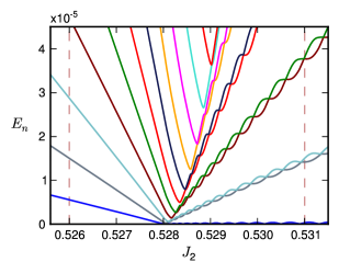
Figure 12: (Color online.) The excitation spectrum with open boundary conditions in the variational subspace with $S_{z}^{Tot}=1/2$. The energies of the first few excited states are shown. The ground state energy was set to zero. The values at which the scaling with $N$ is studied in Fig. 14 are indicated by dashed vertical lines. The data was taken for a chain with 601 sites.

While the on-site magnetization could relatively easily be understood from the results obtained with PBC, this is not the case for the energy spectrum. To the left of the transition ($J_{2}<J_{2}^{L}$), the spectrum for OBC (shown Fig. 12) looks exactly like the spectrum for PBC (shown Fig. 7) – yet there is an important difference: the spectrum for OBC is not degenerate. Introducing the boundary splits the degenerate states. On the other side of the transition ($J_{2}>J_{2}^{L}$), the behavior of the energy of the first excited state also looks familiar: it hits the ground state energy, grows, approaches it again and another level-crossing occurs. Repeated level-crossings of just the two states follow. Higher excitation-levels, however, do not cross many other levels as they do for PBC. They approach the ground state, then turn around and form a pair with the state they would have been degenerate with under PBC. The two states exhibit a repeated pattern of intertwining level-crossings while their mean energy-difference to the ground state grows. We do not know of an intuitive way of understanding the spectrum for OBC from the spectrum with PBC. Modifying the couplings at the boundary of the chain by a multiplicative factor of $\lambda$ and varying $\lambda$ between 0 and 1 we have studied the cross-over from PBC to OBC. A low-energy spectrum similar to the one for OBC is observed until $\lambda\approx 0.9$.

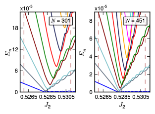
Figure 13: (Color online.) Spectrum with open boundary conditions for chains of 301 and 451 sites. The values at which the scaling with $N$ is studied in Fig. 14 are indicated by dashed vertical lines.

It is reasonable to ask if the Lifshitz point is a well defined point in the spectrum. In order to answer this question we show results in Fig. 13 for chains of length 301 and 451 sites for a range of $J_{2}$ close to $J_{2}^{L}$. As can be clearly seen, the minima of the higher energy levels occur much closer to the first level crossing of the ground state for $N=451$ than for $N=301$. In the thermodynamic limit we expect the minima for all higher lying levels to occur at $J_{2}^{L}$.

We next focus on the scaling of the energy levels with $N$. In Fig. 14(a) we show data for $N^{2}E_{n}$ taken at $J_{2}=0.526$, to the left of the transition as indicated in Fig. 12 and 13. As can be seen, it converges to a constant value indicating that for this value of $J_{2}$ $E_{n}\propto N^{-2}$. For the first excited state this behavior is apparent for quite short chains already and it seems plausible that for higher excited states longer chains would lead to the same decay proportional to $N^{-2}$. This scaling is not surprising since the soliton behaves like a massive particle in a box. We therefore expect the low energy spectrum to be approximated by $\hbar^{2}k^{2}/(2\Delta_{sol})$ with $k=\pi n/2N$, $n=1,2..$, yielding the expected scaling of the energies as $N^{-2}$.

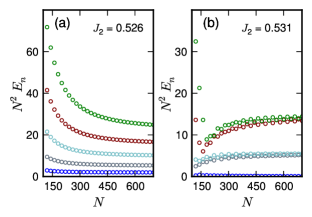
Figure 14: (Color online.) The energy scales proportionally to $N^{-2}$. Plot of $N^{2}\Delta E_{n}$ to the left of the transition (a) and to the right of the transition (b) for the first five excited states.

In Fig. 14(b) we show data taken on the other side of $J_{2}^{L}$ at $J_{2}=0.531$ (again indicated in Fig. 12 and 13). For the smallest $N$ shown, the higher excited states still show signs of the transition at this value of $J_{2}$. For short chains the second, third, forth and fifth excited state thus have minimum in Fig. 14(b). For chains with more than roughly 160 sites we see of intertwining pairs of states familiar from Figs. 12 and 13. The average energy of the pair at big $N$ also scales proportionally to $N^{-2}$. We therefore conclude that sufficiently far away from the transition point for the first few energy-states $\Delta E_{n}\propto J_{2}/N^{2}$.

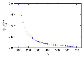
Figure 15: (Color online.) The energy at which the 2^nd excited state turns around goes to zero faster than $N^{-2}$. The value of $J_{2}$ of $E_{2}^{\mathrm{min}}$ was found up to $\Delta J_{2}=10^{-5}$. The resulting uncertainty of the value of the minimum energy is smaller than the size of the symbols in the plot.

In order to study the scaling of the spectrum at the Lifshitz point $J_{2}^{L}$ we focus on the minimum in the second excited state. Although this minimum occurs at slightly different $J_{2}$ as $N$ is varied it serves as the best possible definition of an excited energy scale at the Lifshitz point. Specifically, we define the minimal energy-difference of the ground state and the second excited state as $E^{\mathrm{min}}_{2}=\mathrm{min}_{J_{2}}[E_{2}-E_{0}]$. Our results for $E^{\mathrm{min}}_{2}$ are shown in Fig.15. As can be clearly seen in this figure $E^{\mathrm{min}}_{2}$ goes to zero faster than $N^{-2}$ violating the simple scaling found elsewhere.

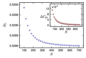
Figure 16: (Color online.) Main panel: $J_{2}^{L}$ as a function of the length of the chain. Inset: The difference between $J_{2}^{L}$ and the $C_{2}$ at which the minimum of the second excited state occurs. All values were determined up to $\Delta J_{2}=10^{-5}$. The resulting uncertainty of the value of the minimum energy is smaller than the size of the symbols in the plot and causes deviations from very smooth behavior.

We now turn to an estimate of the location of $J_{2}^{L}$ within the variational approach. The level-crossing of the first excited and the ground state allows for an easy way to define the value of $J_{2}^{L}$ for a given $N$. As one could already see in the Figures 12 and 13, $J_{2}^{L}$ varies slightly with the length of the chain. Our results are shown in Fig. 16 for chains out to $N=701$. The main panel in Fig. 16 shows that $J_{2}^{L}$ converges to approximately $J_{2}^{L}=0.528$ as one increases the length of the chain.

The value of $J_{2}$ at which the second excited state has its minimum also approaches $J_{2}^{L}$. To show this we use the value of $J_{2}$ at which the $n$-th state reaches its first minimum for a given $N$. We call this quantity $C_{n}$. The inset in Fig. 16 shows $\Delta C_{21}=C_{2}-J_{2}^{L}$. As can be seen, this quantity approaches 0 and the minimum for big $N$ thus lies at the Lifshitz point.

IV Incommensurate behavior in the entanglement entropy

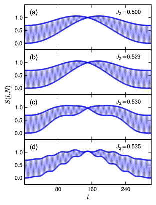
Figure 17: (Color online.) The entanglement entropy of a bipartition of an odd chain. The data was taken for chain of 301 sites and the variational subspace $R_{0}$ (see Sec. II) was used.

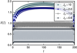
(a) Even number of sites

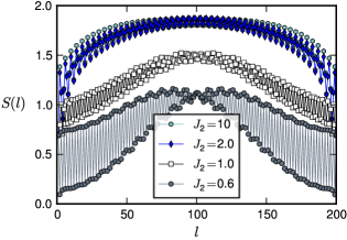
(b) Odd number of sites

Figure 18: (Color online.) The entanglement entropy of a bipartition of an even chain (200 sites) (a) and an odd chain (201 sites) (b). The data was obtained using DMRG with $m=256$ states kept.

The scaling of the entanglement entropy at a (quantum) Lifshitz transition has recently been the subject of interest. Fradkin (2009); Rodney et al. (2012) In free fermion models, analogous to the spin chain model discussed here, the Lifshitz transition is associated with a change in the topology of the Fermi surface. In one dimension new Fermi points appear at the Lifshitz transition and, analogously, new patches appear in higher dimensional models. If one associates a chiral conformal field theory with each patch, it can be argued Swingle (2010) that, when the number of points (patches) increases by a factor $K$, the entanglement should be multiplied with the same factor $K$. For a free fermion model with next nearest neighbor hopping, $t_{2}$, one expects the number of Fermi points to double at the Lifshitz transition $t_{2}^{L}=1/2$ at half-filling with a corresponding doubling in the entanglement entropy. This behavior is well confirmed in numerical calculations. Rodney et al. (2012)

In this section we discuss our results for the entanglement entropy across the Lifshitz point in the odd length $J_{1}$-$J_{2}$ quantum spin chain which is the quantum spin analogue of the model considered in Ref. Rodney et al., 2012. We study the entanglement in terms of the von Neumann entanglement entropy of a sub-system $A$ of size $l$ and reduced density-matrix $\rho_{A}$ defined by von Neumann (1927); Wehrl (1978),

$$S(l,N)\equiv-\mathrm{Tr}[\rho_{A}\ln\rho_{A}]\ ,$$ (12)

where $N$ again stands for the total system size. We consider exclusively open boundary conditions.

If one uses the restricted space $R_{0}$, which was introduced in Sec. II, as the variational subspace, one can also calculate the entanglement entropy using the method employed in this paper. Sørensen et al. (2007) Away from MG and Lifshitz points, where the variational method is not reliable, we complement the variational results with DMRG calculations.

We first discuss the variational results for odd length chains close to the Lifshitz point shown in Fig. 17 for $N=301$. The entanglement entropy at the MG point for the odd length chain, shown in Fig. 17(a), has previously been discussed in detail.  Sørensen et al. (2007) Since the entanglement entropy is very directly connected to the wave function of the state, drastic changes of the wave function should also be present in the entanglement entropy when the Lifshitz point is reached. This is clearly the case as can be seen in Fig. 17. As the Lifshitz point, $J_{2}^{L}$, is reached, the entanglement entropy develops plateaus (Fig.17(c)). As $J_{2}$ is increased more plateaus appear (Fig. 17(d)). For the free fermion model studied in Ref. Rodney et al., 2012 analogous oscillations in the entanglement entropy are observed beyond $t_{2}>1/2$. Because a different subspace was used in the previous parts of this paper, the transition begins at $J_{2}\sim 0.529$ which is slightly higher than $J_{2}\sim 0.528$ which could be inferred from Fig. 13.

For an even length system no such plateaus are visible (see Fig. 18(a)). As $J_{2}\to\infty$ the entanglement increases towards that of two independent gapless Heisenberg chains as it must. A similar increase is seen for an odd number of sites but with pronounced signatures of the incommensurability (see Fig. 18(b)).

V The transition point

The numerical value of $J_{2}^{L}$ for the Lifshitz point depends not only on the length of the chain but also on the basis-set that one uses in the variational calculation. While this is a small concern when one looks at qualitative features, it is of course detrimental if one is interested in a precise estimate of the Lifshitz point. Just using the different basis sets introduced in Sec. II this is evident. Using the smallest basis, $R_{0}$, for a chain with $N=301$ sites, we obtained $J_{2}^{L}\approx 0.5295$ (see Fig. 17) for the onset of oscillations in the entanglement. This is a slightly bigger value than what was found in Fig. 13, $J_{2}^{L}\approx 0.528$, based on the calculations with the larger basis $Z_{s}$.

DMRG can give us a more reliable estimate for $J_{2}^{L}$ at least for small chains. For a chain with $201$ sites we found the first indications of incommensurate behavior in the local magnetization at:

$$J_{2}^{L}\approx 0.538(1)$$ (13)

We expect this estimate to depend on $N$ in roughly the same way as the variational estimate does in Fig. 16. If this is the case, an eventual extrapolation to the $N\to\infty$ limit might change this estimate by 0.0005 which is smaller than the uncertainty to which we have determined the point.

VI Conclusion

We have studied incommensurability effects as they occur in the odd length antiferromagnetic $J_{1}$-$J_{2}$ chain. Even though no exact ground state wave function is known at the MG point, $J_{2}=J_{1}/2$, this point is the disorder point with minimal correlation length. The Lifshitz point $J_{2}^{L}=0.538J_{1}$ marks the onset of significant modulations directly in the ground state $\langle S^{z}_{i}\rangle$ as well as a shift in the ground state momentum. A series of inter-twining level crossings causing the shift in the ground state momentum starts at the Lifshitz point. The shift in the ground state momentum and the associated modulations directly affect the entanglement entropy which shows distinct plateaus developing for $J_{2}>J_{2}^{L}$.

In realistic compounds with chain breaking impurities one would expect half the chain segments to be of odd length. The experimentally well studied compound CuGeO₃ has a $J_{2}\sim 0.36J_{1}<J_{1}/2$.Riera and Dobry (1995) If compounds with a $J_{2}$ in excess of $J_{1}/2$ can be identified, it would be very interesting to experimentally look for the odd length effects that we have detailed here. In particular, the effects on the on-site magnetization shown in Fig. 10 might be observable using NMR techniques or other local probes.

References

References

- Stephenson (1969) J. Stephenson, Canadian Journal of Physics 47, 2621 (1969).
- Stephenson (1970a) J. Stephenson, Phys. Rev. B. 1, 4405 (1970a).
- Stephenson and Betts (1970) J. Stephenson and D. Betts, Phys. Rev. B. 2, 2702 (1970).
- Stephenson (1970b) J. Stephenson, Canadian Journal of Physics 48, 1724 (1970b).
- Stephenson (1970c) J. Stephenson, Canadian Journal of Physics 48, 2118 (1970c).
- Schollwöck et al. (1996) U. Schollwöck, T. Jolicœur, and T. Garel, Phys. Rev. B. 53, 3304 (1996).
- Golinelli et al. (1999) O. Golinelli, T. Jolicoeur, and E. S. Sørensen, Eur. Phys. J. B 11, 199 (1999).
- Bursill et al. (1995) R. Bursill, G. A. Gehring, D. J. J. Farnell, J. B. Parkinson, T. Xiang, and C. Zeng, Journal of Physics: Condensed Matter 7, 8605 (1995).
- Majumdar (1970) C. K. Majumdar, Journal of Physics C: Solid State Physics 3, 911 (1970).
- Lifshitz (1960) I. Lifshitz, Sov. Phys. JETP 11, 1130 (1960).
- Hornreich et al. (1975) R. M. Hornreich, M. Luban, and S. Shtrikman, Phys. Rev. Lett. 35, 1678 (1975).
- Blanter et al. (1994) Y. Blanter, M. Kaganov, A. Pantsulaya, and A. Varlamova, Phys. Rep. 245, 159 (1994).
- Yamaji et al. (2006) Y. Yamaji, T. Misawa, and M. Imada, J. Phys. Soc. Jpn. 75, 094719 (2006).
- Fradkin (2009) E. Fradkin, J. Phys. A: Math. Theor. 42, 504011 (2009).
- Rodney et al. (2012) M. Rodney, H. F. Song, S.-S. Lee, K. Le Hur, and E. S. Sørensen, arXiv:1210.8403 (2012).
- Haldane (1982) F. D. M. Haldane, Phys. Rev. B. 25, 4925 (1982).
- Tonegawa and Harada (1987) T. Tonegawa and I. Harada, Journal of the Physical Society of Japan 56, 2153 (1987).
- Okamoto and Nomura (1992) K. Okamoto and K. Nomura, Physics Letters A 169, 433 (1992).
- Eggert (1996) S. Eggert, Phys. Rev. B 54, R9612 (1996).
- Majumdar and Ghosh (1969) C. K. Majumdar and D. K. Ghosh, Journal of Mathematical Physics 10, 1388 (1969).
- Broek (1980) P. M. v. d. Broek, Physics Letters A 77, 261 (1980).
- Shastry and Sutherland (1981) B. S. Shastry and B. Sutherland, Phys. Rev. Lett. 47, 964 (1981).
- Caspers et al. (1984) W. J. Caspers, K. M. Emmett, and W. Magnus, Journal of Physics A: Mathematical and General 17, 2687 (1984).
- Sørensen et al. (1998) E. S. Sørensen, I. Affleck, D. Augier, and D. Poilblanc, Phys. Rev. B. 58, R14701 (1998).
- Chitra et al. (1995) R. Chitra, S. Pati, H. Krishnamurthy, D. Sen, and S. Ramasesha, Phys. Rev. B. 52, 6581 (1995).
- White and Affleck (1996) S. R. White and I. Affleck, Phys. Rev. B 54, 9862 (1996).
- Uhrig et al. (1999a) G. Uhrig, F. Schönfeld, M. Laukamp, and E. Dagotto, The European Physical Journal B 7, 67 (1999a).
- Sørensen et al. (2007) E. S. Sørensen, M. Chang, N. Laflorencie, and I. Affleck, Journal of Statistical Mechanics: Theory and Experiment 2007, P08003 (2007).
- Affleck et al. (2009) I. Affleck, N. Laflorencie, and E. S. Sørensen, Journal of Physics A: Mathematical and Theoretical 42, 504009 (2009).
- Deschner and Sørensen (2011) A. Deschner and E. S. Sørensen, Journal of Statistical Mechanics: Theory and Experiment 2011, P10023 (2011).
- Hase et al. (1993) M. Hase, I. Terasaki, and K. Uchinokura, Phys. Rev. Lett. 70, 3651 (1993).
- Fagot-Revurat et al. (1996) Y. Fagot-Revurat, M. Horvatić, C. Berthier, P. Ségransan, G. Dhalenne, and A. Revcolevschi, Phys. Rev. Lett. 77, 1861 (1996).
- Fagot-Revurat et al. (1997) Y. Fagot-Revurat, M. Horvatić, C. Berthier, J.-P. Boucher, P. Ségransan, G. Dhalenne, and A. Revcolevschi, Phys. Rev. B. 55, 2964 (1997).
- Horvatić et al. (1999) M. Horvatić, Y. Fagot-Revurat, C. Berthier, G. Dhalenne, and A. Revcolevschi, Phys. Rev. Lett. 83, 420 (1999).
- Uhrig et al. (1999b) G. Uhrig, F. Schönfeld, J.-P. Boucher, and M. Horvatić, Phys. Rev. B. 60, 9468 (1999b).
- Zeng and Parkinson (1995) C. Zeng and J. B. Parkinson, Phys. Rev. B 51, 11609 (1995).
- Nomura and Okamoto (1993) K. Nomura and K. Okamoto, J. Phys. Soc. Jpn. 62, 1123 (1993).
- Nomura and Okamoto (1994) K. Nomura and K. Okamoto, Journal of Physics A: Mathematical and General 27, 5773 (1994).
- Kolezhuk et al. (1996) A. Kolezhuk, R. Roth, and U. Schollwöck, Phys. Rev. Lett. 77, 5142 (1996).
- Roth and Schollwöck (1998) R. Roth and U. Schollwöck, Phys. Rev. B. 58, 9264 (1998).
- Polizzi et al. (1998) E. Polizzi, F. Mila, and E. S. Sørensen, Phys. Rev. B. 58, 2407 (1998).
- Garel and Maillard (1986) T. Garel and J. M. Maillard, J. Phys. C 19, L505 (1986).
- Fáth and Sütő (2000) G. Fáth and A. Sütő, Phys. Rev. B 62, 3778 (2000).
- Nomura (2003) K. Nomura, J. Phys. Soc. Jpn. 72, 476 (2003).
- Arovas and Girvin (1992) D. P. Arovas and S. M. Girvin, “Recent progress in many body theories iii,” (Plenum, New York, 1992) pp. 315–345.
- Hornreich and Bruce (1978) R. Hornreich and A. Bruce, Journal of Physics A: Mathematical and General 11, 595 (1978).
- Hornreich (1980) R. Hornreich, Journal of Magnetism and Magnetic Materials 15, 387 (1980).
- Michelson (1977a) A. Michelson, Phys. Rev. B. 16, 577 (1977a).
- Michelson (1977b) A. Michelson, Phys. Rev. B. 16, 585 (1977b).
- Michelson (1977c) A. Michelson, Phys. Rev. B. 16, 5121 (1977c).
- Eggert et al. (2002) S. Eggert, I. Affleck, and M. Horton, Phys. Rev. Lett. 89, 047202 (2002).
- Nomura and Murashima (2005) K. Nomura and T. Murashima, J. Phys. Soc. Jpn 74, 42 (2005).
- Swingle (2010) B. Swingle, Phys. Rev. Lett. 105, 050502 (2010).
- von Neumann (1927) J. von Neumann, Nachr. Ges. Wiss. Göttingen, 273 (1927).
- Wehrl (1978) A. Wehrl, Rev. Mod. Phys. 50, 221 (1978).
- Riera and Dobry (1995) J. Riera and A. Dobry, Phys. Rev. B 51, 16098 (1995).