Jovian plasma torus interaction with Europa. Plasma wake structure and effect of inductive magnetic field: 3D Hybrid kinetic simulation

Abstract

The hybrid kinetic model supports comprehensive simulation of the interaction between different spatial and energetic elements of the Europa moon-magnetosphere system with respect a to variable upstream magnetic field and flux or density distributions of plasma and energetic ions, electrons, and neutral atoms. This capability is critical for improving the interpretation of the existing Europa flyby measurements from the Galileo Orbiter mission, and for planning flyby and orbital measurements (including the surface and atmospheric compositions) for future missions. The simulations are based on recent models of the atmosphere of Europa (Cassidy et al., 2007; Shematovich et al., 2005). In contrast to previous approaches with MHD simulations, the hybrid model allows us to fully take into account the finite gyroradius effect and electron pressure, and to correctly estimate the ion velocity distribution and the fluxes along the magnetic field (assuming an initial Maxwellian velocity distribution for upstream background ions). Photoionization, electron-impact ionization, charge exchange and collisions between the ions and neutrals are also included in our model. We consider the models with $O^{++}$ and $S^{++}$ background plasma, and various betas for background ions and electrons, and pickup electrons. The majority of $O_{2}$ atmosphere is thermal with an extended non-thermal population (Cassidy et al., 2007). In this paper we discuss two tasks: (1) the plasma wake structure dependence on the parameters of the upstream plasma and Europa’s atmosphere (model I, cases (a) and (b) with a homogeneous Jovian magnetosphere field, an inductive magnetic dipole and high oceanic shell conductivity); and (2) estimation of the possible effect of an induced magnetic field arising from oceanic shell conductivity. This effect was estimated based on the difference between the observed and modeled magnetic fields (model II, case (c) with an inhomogeneous Jovian magnetosphere field, an inductive magnetic dipole and low oceanic shell conductivity).

Keywords: Europa, Jovian magnetosphere, Plasma, Magnetic fields, Ion composition

^∗ Corresponding author. NASA GSFC, Code 673, Bld. 21, Rm. 247, 8800 Greenbelt Rd., Greenbelt, MD 20771, USA. Tel.: +1 301 286 0906; fax: +1 301 286 1648.

E-mail address: Alexander.Lipatov-1@nasa.gov, alipatov@umbc.edu (A.S. Lipatov), John.F.Cooper@nasa.gov (J.F. Cooper), William.R.Paterson@nasa.gov (W.R. Paterson), Edward.C.Sittler@nasa.gov (E.C. Sittler Jr.), Richard.E.Hartle@nasa.gov (R.E. Hartle), David.G.Simpson@nasa.gov (D.G. Simpson)

1.  Introduction

The interaction of the Jovian plasma torus with Europa and other moons is a fundamental problem in magnetospheric physics (see e.g., Goertz, 1980; Southwood et al., 1980; Southwood et al., 1984; Wolf-Gladrow et al., 1987; Ip, 1990; Schreier et al., 1993; Lellouch, 1996). The plasma environment near Europa was studied by flyby observations during the Galileo prime mission and the extended Galileo Europa mission (Kivelson et al., 1997; Khurana et al., 1998; Kivelson et al., 1999, Paterson et al., 1999).

Europa, one of the icy moons of Jupiter, was encountered by the Galileo satellite three times during its primary mission, seven times during its Galileo Europa Mission (GEM), and once during Galileo Millennium Mission (GMM). Europa is located at a radial distance of 9.4 $R_{J}$ (Jovian radii, 71,492 km) from Jupiter, and has a radius of 1560 km (1 $R_{E}$).

The interaction of Europa with the magnetized plasma of the Jovian plasma sheet gives rise to a so-called Alfvén wing, which has been extensively studied in the case of Io (e.g., Neubauer, 1980; Southwood et al., 1980; Herbert, 1985; Lipatov and Combi, 2006). Neubauer (1998; 1999) has shown theoretically how an Alfvén wing is modified by an induced magnetic field, such as that found at Europa (Kivelson et al., 2000). Observations by Kivelson et al. (1992) show the generation of ultra-low frequency electromagnetic waves in Europa’s wake. These waves have frequencies near and below the gyrofrequencies of the ion species in the plasma torus (e.g., ionized sulfur, oxygen, and protons). Ion cyclotron waves grow when ion distribution functions are sufficiently anisotropic, as occurs when ion pickup creates a ring distribution of ions (in velocity space). The analysis of these waves has been done by Huddleston et al. (1997) (Io), Volwerk et al. (2001) and Kivelson, Khurana and Volwerk (2009) (Europa). They found intensive wave power at low frequencies (near and below the cyclotron frequencies of heavy ions) in Europa’s wake during the E11 and E15 flybys. However, our current 3D hybrid modeling cannot yet produce these waves due to insufficient spatial grid resolution.

The most general and accurate theoretical approach to this problem would require the solution of a nonlinear coupled set of integro-MHD/kinetic-Boltzmann equations which describe the dynamics of Jupiter’s corotating magnetospheric plasma, pickup ions, and ionosphere, together with the neutrals from Europa’s atmosphere. To first order, the plasma and neutral atoms and molecules are coupled by charge exchange and ionization. The characteristic scale of the ionized components is usually determined by the typical ion gyroradius, which for Europa is much less than characteristic global magnetospheric scales of interest, but which may be comparable to the thickness of the plasma structures near Europa. Kinetic approaches, such as Direct Simulation Monte Carlo, have been applied to the understanding of global aspects of the neutral atmosphere (Marconi et al., 1996; Austin and Goldstein, 2000). Plasma kinetic modeling is, however, much more complicated, and even at the current stage of computational technology require some approximations and compromises to make some initial progress. Several approaches have been formulated for including the neutral component and pickup ions self-consistently in models that describe the interaction of the plasma torus with Europa.

There have been recent efforts to improve and extend the pre-Galileo models for Europa, Io and Ganymede, both in terms of the MHD (Kabin et al., 1999; Combi et al., 1998; Linker et al., 1998; Kabin et al., 2001; Jia et al., 2008), the electrodynamic (Saur et al., 1998; Saur et al., 1999; Schilling et al., 2008), and hybrid kinetic (Lipatov and Combi, 2006; Lipatov et al., 2010) approaches. These approaches are distinguished by the physical assumptions that they include. MHD and hybrid kinetic models cannot, at least yet, include the charge separation effects which are likely to be important very close to the moon where the neutral densities are large and the electric potential can introduce non-symmetric flow around the body. MHD models for Io either include constant artificial conductivity (Linker et., 1998) or assume perfect conductivity (Combi et al., 1998). Comparisons of the sets of published results do not indicate that this choice has any important consequences. The MHD model of Europa developed by Kabin et al. (1999) includes an exospheric mass loading, ion-neutral charge exchange, and recombination. Further development of this model by Liu et al. (2000) already includes a possible intrinsic dipole magnetic field of Europa. Schilling, Neubauer and Saur (2007; 2008) found that a conductivity of Europa’s ocean of 500 mS/m or largecombined with an ocean thickness of 100 km or smaller is most suitable for explaining the magnetic flyby data. They also found that the influence of the fields induced by the time variable plasma interaction is small compared to the induction caused by the time-varying background field.

Hybrid kinetic models can include the finite ion gyroradius effects, non-Maxwellian velocity distribution for ions, and correct flux of pickup ions along the magnetic field. Hybrid modeling of Io has demonstrated several features. The kinetic behavior of ion dynamics reproduces the inverse structure of the magnetic field (due to drift current) which cannot be explained by standard MHD or electrodynamic modeling which do not account for anisotropic ion pressure. The diamagnetic effect of non-isotropic gyrating pickup ions broadens the B-field perturbation and produces increased temperatures in the flanks of the wake, as observed by the Galileo spacecraft, but had not been explained by previous models. The temperatures of the electrons which are created and cooled by collisions with neutrals in the exosphere and inside the ionosphere may strongly affect the pickup ion dynamics along the magnetic field and consequently the pickup distribution across the wake. The physical chemistry in Io’s corona was considered in the paper by Dols et al. (2008). They couple a model of the plasma flow around Io with a multi-species chemistry model and compare the model results to the Galileo observation in Io’s wake.

Galileo flyby measurements E4, E6 (plasma only), E11, E12, E14, E15, E19, and E26 demonstrate several features in the plasma environment: Alfvén wing formation and an induced magnetosphere, possible existence of the dipole-type induced magnetic field, and variation of the magnetic field in the plasma wake due to diamagnetic currents. The measurements also demonstrate mass loading of the plasma torus plasma by pickup ions and the interaction of the ions with the surface of Europa. For an interpretation of these data we need to use a kinetic model because of effects of the finite ion gyroradius.

Hybrid models have been shown to be very useful in studying the complex plasma wave processes of space, astrophysical, and laboratory plasmas. These models provide a kinetic description of plasmas in local regions, together with the possibility of performing global modeling of the whole plasma system. Revolutionary advances in computational speed and memory are making hybrid modeling of various space plasma problems a much more effective general tool.

In this paper, we apply a time-dependent Boltzmann equation (a “particle in cell” approach) together with a hybrid kinetic plasma (ion kinetic) model in three spatial dimensions (see, e.g. Lipatov and Combi, 2006; Lipatov et al., 2010), using a prescribed but adjustable neutral atmosphere model for Europa. A Boltzmann simulation is applied to model charge exchange between incoming and pickup ions and the immobile atmospheric neutrals. In this paper we discuss the results of the hybrid kinetic modeling of Europa’s environment - namely, the global plasma structures (formation of the magnetic barrier, Alfvén wing, pickup ion tail etc.). The results of these kinetic modeling are compared with the Galileo E4 flyby observational data. Currently, we are working on the hybrid model of the E12 flyby. The remarkable aspect of this flyby is a strong variation in the upstream plasma density profile approximately from 400 cm^-3 to 80 cm^-3. The results of this modeling will be discussed in future publications.

The paper is organized as follows: in Section 2 we present the computational model and a formulation of the problem. In Section 3 we present the results of the modeling of the plasma environment near Europa and the comparison with observational data. Finally, in Section 4 we summarize our results and discuss the future development of our computational model.

2.  Formulation of the Problem and Mathematical Model

To study the interaction of the plasma torus with the ionized and neutral components of Europa’s environment, we use a quasineutral hybrid model for ions and electrons. The model includes ionization (which in the Europa environment is dominated by electron impact ionization, not photoionization) and charge exchange. The atmosphere is considered to be an immobile component in this paper.

In our hybrid modeling, the dynamics of upstream ions and implanted ions are described in a kinetic approach, while the dynamics of the electrons are described in a hydrodynamical approximation. The details of this plasma-neutral approach were developed early for the study of the Io-Jovian plasma interaction (Lipatov and Combi, 2006).

The single ion particle motion is described by the equations (see, e.g. Eqs. (1) and (14) from Mankofsky, Sudan and Denavit (1987)):

$${{d{\bf r}_{s,l}}\over{dt}}={\bf v}_{s,l};\quad{{d{\bf v}_{s,l}}\over dt}=\frac{e}{M_{\mathrm{i}}}\left({\bf E}+\frac{{\bf v}_{s,l}\times{\bf B}}{c}\right)-\frac{m_{e}\nu_{ie}}{M_{i}}({\bf v}_{s,l}-{\bf U}_{i})-\frac{m_{e}\nu_{ie}}{M_{i}en_{i}}{\bf J}-\nu_{io}{\bf v}_{s,l}.$$ (1)

Here we assume that the charge state is $Z_{i}=1$. ${\bf U}_{i}$, and ${\bf J}$ denote the charge-averaged velocity of all (incoming and pickup) ions and the total current, Eq. (5). The subscript $s$ denotes the ion population ($s=1,2$ for incoming ions and $s=3,4$ for pickup ions) and the index $l$ is the particle index. $\nu_{ie}$ and $\nu_{io}$ are collision frequencies between ions and electrons, and ions and neutrals that may include Coulomb collisions and collisions due to particle-wave interaction.

For a plasma, the thermal velocity, $v_{\alpha}^{\prime}$ ($\alpha=i,e$), is assumed greater than the drift velocity, so we take

$$\nu_{\alpha,o}=n_{o}\sigma^{o,\alpha}v_{\mathrm{\alpha}}^{\prime},$$ (2)

where the cross section $\sigma^{o,\alpha}$ is typically about $5\times 10^{-15}$ cm² (see, e.g., Eq. (17) from Mankofsky, Sudan and Denavit (1987)).

For massless electrons the equation of motion of the electron fluid takes the form of the standard generalized Ohm’s law (e.g. Braginskii, 1965):

$${\bf E}=\frac{1}{en_{\mathrm{e}}c}({\bf J}_{\mathrm{e}}\times{\bf B})-\frac{1}{en_{\mathrm{e}}}\nabla p_{\mathrm{e}}-\frac{m_{\mathrm{e}}}{e}\left[\sum_{s}\nu_{e,s}[({\bf U}_{i}-{\bf U}_{s})-\frac{{\bf J}}{ne}]+\nu_{a,eo}{\bf U}_{e}\right],$$ (3)

where $p_{\mathrm{e}}=nm_{\mathrm{e}}\langle v_{\mathrm{e}}^{\prime 2}\rangle/3=n_{\mathrm{e}}k_{B}T_{\mathrm{e}}$, and $v_{\mathrm{e}}^{\prime}$ are the scalar electron pressure and the thermal velocity of electrons, and the electron current is estimated from Eq. ( 5).

The induction equation (Faraday’s law) has a form

$$\frac{1}{c}\frac{\partial{\bf B}}{\partial t}+\nabla\times{\bf E}=0.$$ (4)

The total current is given by

$${\bf J}={\bf J}_{\mathrm{e}}+{\bf J}_{\mathrm{i}};\quad{\bf J}_{\mathrm{i}}=\sum_{s=1}^{2}en_{s}{\bf U}_{s}=en_{i}{\bf U}_{i},$$ (5)

where ${\bf U}_{s}$ is the bulk velocity of ions of the type $s$.

Since we suppose that electron heating due to collisions with ions is very small, the electron fluid is considered adiabatic. For simplicity we assume that the total electron pressure may be represented as a sum of partial pressures of all electron populations:

$$p_{\mathrm{e}}\propto\frac{(\beta_{\mathrm{e}}n_{\mathrm{i,up}}^{5/3}+\beta_{\mathrm{e,PI}}n_{\mathrm{i,PI}}^{5/3})}{\beta_{\mathrm{e}}},$$ (6)

where $\beta_{\mathrm{e}}$ and $\beta_{\mathrm{e,PI}}$ denote electron upwind, and pickup betas. Note that $\beta_{e,k}=p_{e,k}/(B^{2}/8\pi)$, where $k$ is a population of electrons. We also assume here that $n_{\mathrm{e,up}}=n_{\mathrm{i,up}}$, $n_{\mathrm{e,PI}}=n_{\mathrm{i,PI}}$.

The neutral atmosphere of Europa serves as a source of new ions, mainly by electron impact ionization from corotating (or nearly corotating) plasma and also by photoionization. The neutral atmospheric molecules also serve as collisional targets for charge exchange by corotating ions. The impacting ions consist of both upstream torus ions and newly implanted ions which are picked up by the motional electric field.

In the current model we assume that the background plasma contains only ions with molecular mass/charge of 8 and 16 corresponding to $O^{++}$ and $S^{++}$, respectively.

We assume that Europa has a radius $R_{E}=1560$ km. We have also adopted a two-species description for the neutral $O_{2}$ exosphere of exponential form (Shematovich et al., 2005)

$$n_{\mathrm{neutral,k}}\approx n_{\mathrm{atmos,k}}\exp{[-(r-r_{\mathrm{exobase,k}})/h_{atmos,k}]},$$ (7)

where $n_{\mathrm{atmos,k}}$ denotes the maximum value of the neutral density extrapolated to the exobase ($n_{\mathrm{atmos,1}}=3\times 10^{4}$cm^-3; $n_{\mathrm{atmos,2}}=8.5\times 10^{7}$cm^-3; $r_{\mathrm{exobase},1}\approx 1700$ km; $r_{\mathrm{exobase},2}\approx 1560$ km), and index $k$ denotes either non-thermal ($k=1$) or thermal ($k=2$) species. Here the scale heights $h_{\mathrm{atmos,1}}=200$ km and $h_{\mathrm{atmos,2}}=30$ km.

The production rate of new ions from the exosphere near Europa corresponds to

$$G_{\mathrm{exo,k}}\propto\nu_{i,k}n_{\mathrm{atmos,k}}\exp[-(r-r_{\mathrm{exobase},k})/h_{\mathrm{atmos,k}}],$$ (8)

where $n_{\mathrm{atmos,k}}$ denotes the value of the neutral component density at $r=r_{\mathrm{exobase},k}$ and $\nu_{i,k}$ is the effective ionization rate per atom or molecule of species $k$. $\nu_{i,k}$ includes the photoionozation $\nu_{ph}$, and the electron impact ionization by the magnetospheric electrons $\nu_{e,im}$. We assume that our model of the atmosphere mainly consists of $O_{2}$, and we use the effective photoionization rate $1.7\times 10^{-8}$ s^-1 (Johnson et al., 2009). We also adopt the effective electron impact ionization rates of $2.4\times 10^{-8}$ cm³/s (for 20 eV electrons) and $1.1\times 10^{-7}$ cm³/s (for 250 eV electrons) (see e.g. Johnson et al., 2009). Since the hot electrons represent only 5% of the total electron density (see Voyager 1 plasma science (PLS) measurements analyzed by Sittler and Strobel (1987) and Bagenal (1994)) we use the same composition for computing the impact ionization rate. We assume that the Sun is located in the direction opposite the $x$ axis.

The interaction of ions with neutral particles by charge exchange (see Eqs. (12) - (15) from Lipatov and Combi, 2006) currently includes for the following reactions:

$$O^{++}+O_{2}\rightarrow O^{+}+O_{2}^{+}$$

$$S^{++}+O_{2}\rightarrow S^{+}+O_{2}^{+}$$

$$O_{2}^{+}+O_{2}\rightarrow O_{2}+O_{2}^{+}$$ (9)

The effective cross section for charge exchange ($\sigma_{c,ex}=2.6\times 10^{-19}$ m²) was the same as that used in the hybrid modeling of Io’s plasma environment (see Lipatov and Combi, 2006; and McGrath and Johnson, 1989). A more complete list of reactions will be considered in future modeling. Of course, this also requires the addition of Monte Carlo computations. However, this approach is beyond the scope of this paper.

Our code solves equations (1) - (9).

We discuss two models of the interaction between the Jovian magnetosphere and Europa. In Sect. 3.1 we discuss the interaction model for the cases with different ion and electron betas, different pickup ion production rates near the surface of Europa, and a homogeneous global Jovian magnetic field (model I, cases (a) and (b)). In in Sect. 3.2 we consider model II, case (c) with a realistic global Jovian magnetic field and the internal dipole magnetic field placed in the center of Europa. To study the interaction of the plasma torus with the ionosphere of Europa, the following Jovian plasma torus and ionosphere parameters were adopted in accordance with the Galileo Europa E4 flyby observational data (Paterson, Frank and Ackerson, 1999; Khurana et al., 1998; Kivelson et al., 1997; Kivelson et al., 1998): magnetic field, $B_{0}=469$ nT and ${\bf B}=(77.6,-140.7,-441.3)$ nT; torus plasma speed relative to Europa (Paterson, Frank and Ackerson, 1999), $U_{0}=105$ km/s; upstream ion densities, $\rho_{O^{++}}=10$ cm^-3; $\rho_{S^{++}}=10$ cm^-3 and ion temperature, $T_{i}=(25-100)$ eV (Paterson, Frank and Ackerson, 1999); electron temperature for suprathermal population, $T_{e}=20$ eV (Sittler and Strobel, 1987); ratio of specific heats, $\gamma=5/3$; Alfvén and sonic Mach numbers, $M_{A}=0.25$; $M_{s}=3.66$.

Initial Conditions. Initially, the computational domain contains only supersonic and sub-Alfvénic plasma torus flow with a homogeneous spatial distribution and a Maxwellian velocity distribution; the pickup ions have a weak density and spherical spatial distribution. The magnetic and electric fields are ${\bf B=B}_{0}$ and ${\bf E}=-{\bf U}_{0}\times{\bf B}_{0}$. Inside Europa the electromagnetic fields are ${\bf E}=0$ and ${\bf B=B}_{0}$, and the bulk velocities of ions and electrons are also equal to zero. Here the $X$ - axis is directed in the corotation direction, the $Y$ - axis is directed toward Jupiter, and the $Z$ - axis is directed to the north, as shown in Fig. 1. In model I, cases (a) and (b) we use a homogeneous magnetic field for the initial and boundary conditions (see paragraph above). In model II, case (c) we use an extrapolation of the magnetic field profile along the E4 trajectory (see, Kivelson et al., 1999; 2009) onto the computation domain for the initial and boundary conditions. The effect of global variation on the magnetic field in the rest of Europa was not taken into account directly in the modeling but it was included in the modeling as an internal magnetic dipole (see, Schilling et al., 2007; 2008).

At $t>0$ we begin to inject the pickup ions with a spatial distribution according to Eq. (8). Far upstream ($x=-15\,R_{E}$), the background ion flux is assumed to have a Maxwellian velocity distribution.

Boundary Conditions. On the side boundaries ($y=\pm DY/2$ and $z=\pm DZ/2$), periodic boundary conditions were imposed for incoming flow particles. The pickup ions exit the computational domain when they intersect the side boundary surfaces $y=DY/2-5\times\Delta y$, $y=-DY/2+5\times\Delta y$, $z=DZ/2-\times\Delta z$, $z=-DZ/2+5\times\Delta z$. Thus there is no influx of pickup ions at the side boundaries.

At the side boundaries we also use a damping boundary condition for the electromagnetic field (see e.g., Lipatov and Combi, 2006; Umeda, Omura and Matsumoto, 2001). This procedure allows us to reduce outcoming electromagnetic perturbations, which may be reflected at the boundaries.

Far downstream ($x=12\,R_{E}$), we adopted a free escape condition for particles and the “Sommerfeld” radiation condition for the magnetic field (see e.g., Tikhonov and Samarskii, 1963) and a free escape condition for particles with re-entry of a portion of the particles from the outflow plasma.

At Europa’s surface, $r=R_{E}\approx 1560$ km, the particles are absorbed. In model I, there is no boundary condition at Europa’s surface for the electromagnetic field; we also use our equations for the electromagnetic field, (Eqs. (2), (4) and (9) from Lipatov and Combi (2006)) inside Europa but using the low internal conductivity (Reynolds number, $Re=0.5$) and a very small value for the bulk velocity that is calculated from the particles. In model II, we also use an inductive magnetic dipole $(0,0,-72.5)$ nT $R_{E}^{3}$ for the boundary condition at Europa’s surface that simulates the effect of a nonstationary Jovian magnetic field at the position of Europa. In this way the jump in the electric field is due to the variation of the value of the conductivity and bulk velocity across Europa’s surface. (Note that the center of Europa is at $x=0,y=0,z=0$).

The three-dimensional computational domain has dimensions $DX=27\,R_{E}$, $DY=30\,R_{E}$ and $DZ=30\,R_{E}$. We used mesh of $301\times 301\times 271$ grid points, and $5\times 10^{8}$ and $5\times 10^{8}$ particles for ions and pickup ions, respectively, for a homogeneous mesh computation. The particle time step $\Delta t_{p}$ and the electromagnetic field time step $\Delta t_{EB}$ satisfy the following condition: $v_{max}\Delta t_{p}\leq\min(\Delta x,\Delta y,\Delta z)/8$ and $v_{max}\Delta t_{EB}\leq\min(\Delta x,\Delta y,\Delta z)/256$.

The global physics in Europa’s environment is controlled by a set of dimensionless independent parameters such as $M_{\mathrm{A}}$, $\beta_{\mathrm{i}}$, $\beta_{\mathrm{e}}$, $M_{\mathrm{i}}/M_{\mathrm{p}}$, ion production and charge exchange rates, diffusion lengths, and the ion gyroradius $\epsilon=\rho_{\mathrm{ci}}/R_{E}$. Here $\rho_{\mathrm{ci}}=U_{0}/(eB/M_{\mathrm{i}}c)=M_{\mathrm{A}}c/\omega_{\mathrm{pi}}$ and the ion plasma frequency $\omega_{\mathrm{pi}}=\sqrt{4\pi n_{0}e^{2}/M_{\mathrm{i}}}$. $M_{i}$ and $M_{p}$ denote the ion and proton masses. For real values of the magnetic field, the value of the ion gyroradius is about $80$ km, which is calculated from the local bulk velocity. The dimensionless ion gyroradius and grid spacing have the values $\epsilon=0.05$ and $\Delta_{x}/R_{E}=0.1$.

In order to study ion kinetic effects (e.g. excitation of low-frequency oscillations ($\omega<<\Omega_{b}$) by mass loading), we must satisfy the condition $\Delta\leq(10-20)c/\omega_{pb}$, where $\Omega_{b}$ and $\omega_{pb}$ denote the gyrofrequency and plasma frequency for upstream ions (Winske et al., 1985). The above estimation of the plasma parameters shows that we have good resolution for the low-frequency waves (see also Lipatov et al, 2012).

There is another problem - numerical resolution of the gyroradius on the spatial grid. This becomes very important near Europa’s surface where the MHD model cannot to be used and we have to use a kinetic model to study the trajectory of heavy ions and their interaction with the surface of Europa. Our current model still does resolve this last effect and we expect to improve the model by use of a spherical system of coordinates in future research.

3.  Results of Europa’s Environment Simulation

3.1  Effects of plasma betas on the plasma wake structure

In order to study the effect of plasma parameters on the structure of the plasma wake and the Alfvén wing, we have performed modeling (model I) for two cases (a) and (b) with different values of the upstream background ion temperatures, pickup electron temperatures, and a value of the pickup production rate near the surface of Europa.

The following plasma parameters are chosen the same for both models: full magnetosphere corotation speed is $U_{0}=105$ km/s; upstream densities are $\rho_{O^{++}}=10$ cm^-3, $\rho_{S^{++}}=10$ cm^-3; magnetic field is $B_{0}=469$ nT; ${\bf B}=(77.6,-140.7,-441.3)$ nT; Alfvénic Mach number $M_{A}=0.25$; magnetosonic Mach number $M_{s}=3.66$. The model of $O_{2}$ atmosphere was taken from Cassidy et al. (2007), Shematovich et al. (2005) and Smyth and Marconi (2006). In model I, cases (a) and (b), Europa’s interior is represented as low conducting body with Reynolds number $Re=0.5$.

Model I, case (a): upstream ion temperatures are $T_{O^{++}}=25$ eV; $T_{S^{++}}=25$ eV and upstream electron temperature is $T_{e,0}=20$ eV. Temperatures of electrons connected with non-thermal and thermal $O_{2}^{+}$ pickup ions are $T_{e,non-thermal}=20$ eV; $T_{e,thermal}=20$ eV.

Model I, case (b) (reduced density for thermal $O_{2}$ by a factor 60 near surface and higher electron temperatures; increased upstream ion temperatures, $T_{O^{++}}=100$ eV; $T_{S^{++}}=100$ eV): the upstream electron temperature is $T_{e,0}=20$ eV; temperatures of electrons connected with non-thermal and thermal $O_{2}^{+}$ pickup ions $T_{e,non-thermal}=200$ eV; $T_{e,thermal}=200$ eV.

We have computed several hybrid models with different ion and electron betas, and different production rate for $O_{2}^{+}$ pickup ions, but we discuss here only the models that fit the observations.

The initial thermal velocities of $O_{2}^{+}$ non-thermal and thermal ions are chosen as the following: $v_{th,non-thermal}=3.0$ km/s (2 eV) and $v_{th,thermal}=0.5$ km/s (0.05 eV). The initial bulk velocity of $O_{2}^{+}$ pickup ions is about 1 km/s. Eq. 8 gives the following total pickup ion production rate: $Q_{O_{2}^{+},thermal}=0.825\times 10^{28}\,s^{-1}$ and $Q_{O_{2}^{+},non-thermal}=1.95\times 10^{26}\,s^{-1}$.

Let us consider first the global picture of the interaction of the plasma torus with Europa. The results of this modeling are shown in Figs. 2, 3, and 4. Figures 2 and 3 demonstrate 2D cuts for non-thermal and thermal $O_{2}^{+}$ pickup ion density profiles. One can observe the asymmetrical distribution of the pickup ion density (top, case (a)) and (bottom, case (b)) in the $x$-$y$, $y$-$z$ $(x=5\,R_{E})$ and $z$-$x$ planes. The pickup ion motion is determined mainly by the electromagnetic drift. The motion along the magnetic field is due to the thermal velocity and the gradient of the electron pressure. A more wider density profile of the pickup ions was observed in the case (b), Figs. 2 and 3 (bottom).

The figures demonstrate a strong structuring in the non-thermal and thermal $O_{2}^{+}$ ion density profiles. While case (a) produces a much higher peak in the thermal $O_{2}^{+}$ ion density as was seen in E4 observations, case (b) produces much better agreement with observation for the thermal $O_{2}^{+}$ ion density as shown in Figs. 2 and 3.

The modeling also demonstrates the asymmetrical distribution of the background $O^{++}$ ion density in the $x$-$y$, $y$-$z$ $(x=5\,R_{E})$ and $z$-$x$ planes, Fig. 4. The asymmetrical distribution of the background ions in the $x$-$y$ plane may be explained by the existence of a strong $B_{z}$ component in the upstream magnetic field. One can also see an increase in the plasma density near Europa due to the formation of a magnetic barrier (not shown here). In case (b) this effect is stronger than in case (a). The density profiles for $SO^{++}$ background ions are close to the density profiles for $O^{++}$ ions.

The inclination of the magnetic field results in an asymmetrical boundary condition for ion dynamics (penetration and reflection) in Europa’s ionosphere and an asymmetrical Alfvén wing.

Note that the background ion flow around the effective obstacle that is produced by pickup ions and the ionosphere. The pickup ions flow from the “corona” across the magnetic field due to electromagnetic drift, whereas the motion along the magnetic field is determined by the thermal velocity of ions and the electron pressure.

Figure 5 demonstrates the 1D cuts ($y=0$, $z=0$) of the background density $O^{++}$ for case (a) (top) and case (b) (bottom). Strong jumps in the plasma density with $N_{O^{++},max}=80$cm ^-3 (case (a)) and $N_{O^{++},max}=17$cm ^-3 (case (b)) are observed on the day-side of the ionosphere, whereas a reduction in the plasma density is observed in the plasma wake. Note that the jump in the plasma density profile is stronger in case (a) than it is in case (b). Both jumps are located near the surface of Europa.

Figures 6 shows 1-D density profiles of the background and pickup ions along the E4 trajectory of the Galileo spacecraft. One can see a strong plasma void in the center of the plasma wake. There is also a sharp boundary with an overshoot in the density profiles on the side of the plasma wake in the Jupiter-direction, and a smooth boundary layer on the side in the anti-Jupiter direction, Fig. 6 (top). The density profile for $O^{++}$ is similar the density profiles for the $S^{++}$ upstream ions. Fig. 6 (middle and bottom) also shows the density profiles for the non-thermal (top) and thermal (bottom) $O_{2}^{+}$ pickup ions. One can see the split structure of the plasma tail. The effect of splitting of the plasma tail was also observed in the hybrid modeling of weak comets (see, e.g., Lipatov, Sauer and Baumgätel, 1997; Lipatov, 2002). The general feature of this plasma density is due to the effect of the finite heavy gyroradius. The total ion density profile observed in E4 pass is shown in Fig. 6 (bottom). The observed value of the density in these peaks is lower than in modeling and it may be explained by an overestimated density of $O_{2}^{+}$ pickup ions for case (a). In the case (b), disagreement is not as strong, an improvement of the atmosphere model is still required.

The modeling gives the following total fluxes for the $O_{2}^{+}$ pickup ions (case (a)): $1.4\times 10^{22}$ mol/s (non-thermal) and $1.75\times 10^{25}$ mol/s (thermal); (case (b)): $0.8\times 10^{22}$ mol/s (non-thermal) and $1.0\times 10^{25}$ mol/s (thermal) across the back boundary $x=12R_{E}$.

Let us consider a global distribution of the electric and magnetic field in Europa’s environment. Figure 7 shows $B_{x}$, $B_{z}$ magnetic and $E_{y}$ electric field profiles for case (a) (left) and case (b) (right). The $y-z$ cuts (top and middle) are located at $x/R_{E}=7$, and $x-y$ cuts (bottom) are located at $y=0$. The figure demonstrates perturbations in the magnetic $B_{x}$ and electric $E_{y}$ field profiles, which are due to the formation of an Alfvén wing. The increase in the magnetic field $B_{z}$ indicates the formation of an asymmetrical magnetic barrier, Fig. 7 (bottom).

The asymmetry of the modeling distributions in ${\bf B}$ appears to be caused by the finite gyroradius effects of incoming and pickup ions. A weak perturbation of the magnetic field was observed near the ionosphere of Europa: compression of the upstream magnetic field and decompression in the plasma wake.

The modeling also shows the formation of an Alfvén wing in the direction of the main magnetic field. The formation of the Alfvén wing in a sub-Alfvénic flow near Europa is similar to a formation near Io, which was first studied analytically by Neubauer (1980). The pickup ions play an important role in the fine structure of the Alfvén wing due to effects of mass loading. In particular, the scale of the front of the Alfvén wing must be determined by the gyroradius of pickup ions. Unfortunately, in our 3D hybrid kinetic simulation we cannot yet resolved these spatial scales.

3.2  Effects of inductive Europa’s magnetic field

In the first set of models (Sect. 3.1, model I, cases (a) and (b)), we used a homogeneous global magnetic field as an initial condition. These models do not produce agreement between the simulated and observed magnetic fields.

In the second set of modeling we take into account the gradient of the global Jovian magnetic field for an initial magnetic field distribution. In the paper by Kivelson, Khurana, Stevenson et al. (1999); Kivelson et al. (1997); Kivelson et al. (2000), it has been shown that the $B_{y}$ component of the magnetospheric magnetic field has strong time variations at the position of Europa. In the MHD-fluid approximation the effects of such magnetic field variations are estimated in Schilling, Neubauer and Saur (2007); Schilling, Neubauer and Saur (2008). The initial plasma density and bulk velocity distribution in our modeling were taken from the E4 flyby data (Paterson et al., 1999).

We created the following model II, case (c) for simulation: the density for thermal $O_{2}$ is the same as for model I, case (b), and the pickup electron temperature is lower than in model I, case (b). The plasma density and bulk velocity distribution in our modeling were taken from the E4 flyby data (Paterson et al., 1999): full magnetosphere corotation speed $U_{0}=105$ km/s; upstream densities are $\rho_{O^{++}}=10$ cm^-3; $\rho_{S^{++}}=10$ cm^-3; upstream ion and electron temperatures, $T_{O^{++}}=100$ eV; $T_{S^{++}}=100$ eV; $T_{e,0}=20$ eV. The temperatures of electrons connected with non-thermal and thermal $O_{2}^{+}$ pickup ions are $T_{e,non-thermal}=100$ eV; $T_{e,thermal}=100$ eV.

In our hybrid kinetic modeling (model II) we use a simple magnetic dipole model of the induced oceanic magnetic field from the ten-hour corotation variation of the background Jovian magnetic field at Europa (see paragraph “Boundary Conditions”, Sect. 2). And, finally, we fit the results of modeling to the components of the measured magnetic field.

This is not yet a fully self-consistent approach but provides a first approximation. Also, the ocean may not be exactly a spherically symmetric conducting shell and may ultimately require a higher-order multipole model for the induced fields.

Figure 8 demonstrates the 2D cuts for non-thermal and thermal $O_{2}^{+}$ pickup ion densities. The figure does not show any extension of the pickup ion profile in the $y$ and $z$ directions. The plasma wake is narrower in the $y$ and $z$ directions compared to that produced by model I, cases (a) and (b). The reason for this effect is the lower temperature of electrons connected with pickup $O_{2}^{+}$ ions than in case (b), and a lower pickup ion production rate near the surface of Europa than in case (a).

Figure 9 shows the distribution of the $O^{++}$ ion density in the $x$-$y$, $y$-$z$ $(x=5\,R_{E})$ and $z$-$x$ planes. The narrow plasma wake may be explained by the cooler temperature of the electrons connected with $O_{2}^{+}$ pickup ions, resulting in a smaller polarization electric field that is responsible for the expansion of Europa’s ionosphere.

One can also see an increase in the plasma density near Europa due to the formation of a magnetic barrier (not shown here). The density profile for $SO^{++}$ background ions is close to the density profile for $O^{++}$ ions as in model I, cases (a) and (b).

Figure 10 shows a 1-D cut of the background $O^{++}$ density along the $x$- axis ($y=0,z=0$). One can see jump in the background plasma density with $N_{O^{++},max}=90$cm^-3 (model II, case (c)) on the day-side of the ionosphere and depletion in the plasma density in Europa’s plasma wake. Note that the jump in the plasma density profile is stronger in model II, case (c) than is observed in model I, case (a). The jump is located near the surface of Europa, as was observed in model I, cases (a) and (b).

Figures 11 shows 1-D density profiles of the background and pickup ions along the E4 trajectory of the Galileo spacecraft. One can see a strong plasma void in the center of the plasma wake. There is also a sharp boundary with an overshoot in the density profiles on the left side of the plasma wake, and a smooth boundary layer on the right side, Fig. 11 (top). The density profile for $S^{++}$ is similar the density profile for $O^{++}$ background ions. Fig. 10 (middle) shows the density profiles for non-thermal and thermal $O_{2}{+}$ pickup ions. The total ion density profile observed during the E4 pass is shown in Fig. 11 (bottom). Again, one can see two peaks in the total ion density profile. However, the observed value of the density in these peaks is lower than predicted by the model; this may be explained by an overestimated density of $O_{2}^{+}$ pickup ions for model II, case (c).

The modeling shows that the shape of Europa’s global plasma environment depends on a combination of the upstream plasma parameters and pickup ion and electron parameters. For example, reducing in the temperature of electrons connected with pickup ions results in a higher density of thermal $O_{2}^{+}$ pickup ions at the trajectory of the spacecraft (compare Fig. 6 (right) and Fig. 11). This effect is connected with the polarization electric field which is proportional to the gradient of the electron pressure. Reducing the temperature of the background upstream ions results in the widening of the plasma wake (compare Fig. 6 (left and right, top) and Fig. 11 (top)). These effects were earlier demonstrated in the 3-D hybrid simulation of Io’s plasma environment (Lipatov and Combi, 2006). We have found the similarities between the plasma environments of these objects. Indeed, Io and Europa have sufficiently thin exospheres and strong magnetic fields resulting in a small value of the ion gyroradius.

Let us consider the global distribution for the electromagnetic field of model II, case (c). Figure 12 shows 2-D cuts for the magnetic $B_{x}$, $B_{z}$ and electric $E_{y}$ field profiles. The distributions for the $B_{z}$, $E_{y}$ field shown in the figure are close to the distributions for model I, case (b). However, there are significant differences between the $B_{x}$ profiles for model I, case (a) and case (b), and model II, case (c). The differences between the $B_{x}$ profiles for cases (a) and (b), Fig. 7 (top) are due to a much higher density of the thermal $O_{2}{+}$ pickup ions in the plasma wake, whereas the differences between the $B_{x}$ profiles for cases (b) and (c) are due to the nonlinear interaction of the Alfvén wing with the inhomogeneous Jovian magnetic field in model II, case (c).

Figure 13 shows the magnetic field components (solid line) $B_{x}$, $B_{y}$ , $B_{z}$, and $|B|$ along the E4 trajectory of the Galileo spacecraft. The magnetic field components of the inductive magnetic dipole that simulates the effect of the nonstationarity of the Jovian magnetic field are shown by a dotted line ($---$). The circles ($\circ$) denote observational data from Kivelson et al. (1997) and the initial Jovian magnetospheric field at the position of Europa (+++). The simulation produces a satisfactory agreement with the observational data for the $B_{y}$ magnetic field component, but not for the $B_{x}$ and $B_{z}$ magnetic field components. A multipole model for the oceanic magnetic field may address this issue. We will need to improve the model of the $O_{2}$ atmosphere, the resolution of the ion trajectory, and the gradient in the atmosphere/ionosphere density profiles near the surface of Europa to obtain better agreement in the $B_{x}$ and $B_{z}$ magnetic field components

4.  Conclusions

Hybrid modeling of Europa’s plasma environment for the E4 encounter with 3 ion species demonstrated several features:

• The modeling shows a strong phase mixing in the plasma wake. The plasma wake demonstrates the formation of time-dependent structuring in the pickup ion tails (see, e.g., McKenzie, Sauer, Dubinin, 2001 for a weak comet case) and the splitting of the pickup ion tails. The splitting of the plasma wake has the same nature as the splitting of the weak comet’s plasma wake or the splitting of Titan’s plasma wake. Such finite gyroradius effects were also observed in 2.5 D hybrid and bi-fluid modeling of a weak comet (see, e.g., Lipatov, Sauer, Baumgärtel, 1997; Sauer et al., 1996; 1997; Lipatov, 2002) and in 3D hybrid modeling of Titan’s plasma environment (Lipatov et al., 2011; 2012). The further investigation of these fine structure needs an additional modeling with much better resolution.

• The model shows a magnetic field barrier formation at the day-side portion of the ionosphere. The formation of an Alfvén wing in the plane of the external magnetic field was also observed. Note that the Alfvén wing was earlier observed in a hybrid simulation of the plasma environment of Io and Europa by Lipatov and Combi (2006) and by Lipatov et al. (2010). An MHD simulation of the plasma environment of Io and Europa also produces the formation of an Alfvén wing (Saur et al., 1999; 1998; Liu et al., 2000; Schilling et al., 2008).

• The ion and electron temperatures play an important role in plasma structure formation, and in creating the ion fluxes inside the ionosphere. These effects were observed earlier in a 3-D hybrid simulation of Io’s plasma environment (Lipatov and Combi, 2006). The hybrid model produces the correct pickup ion flux along the magnetic field, in contrast to the MHD models which operate with pickup ions with a Maxwellian velocity distribution. In the current paper we have presented only three runs with different combinations of the upstream ion and pickup electron temperatures.

• The model’s total ion density in the plasma wake does not satisfactory match the observed density.

• The constant induced dipole moment (model II, case (c)) improves a fit of the magnetic field $B_{y}$ component to the E4 trajectory. However, a fit of the magnetic field $B_{x}$ component is still not satisfactory due to the imperfect model of the atmosphere/ionosphere and unsatisfactory numerical resolution of the gyroradii on the grid cell.

• Use of an inhomogeneous background magnetic field provides a good agreement between the observed and simulated magnetic fields. However, we still need to improve the resolution of the gradient in the atmosphere density, the gyroradius of pickup ions, and the fields in the internal non-conduction ice shell and conduction ocean layers of Europa.

In our future computational models, we plan to include a nonstationary boundary condition for the magnetic field in order to take into account the spatially inhomogeneous and nonstationary background Jovian magnetic field. This model will also be appropriate for a potentially nonspherical ocean shell. We also plan the use of a varying atmospheric density, a varying electron temperature (that plays key-role in the pickup ion dynamics), and sputtering processes (Johnson, 1990; Johnson et al., 1998) at the surface of Europa. We also plan to use a composite grid structure using the “cubed sphere” technique (see, e.g. Koldoba et al, 2002) to improve the resolution of the a small scales near the surface of Europa and to increase the size of the computational domain.

The composite grid structure will allow us to estimate the inductive magnetic field from the ocean as a part of the total current closure that also includes the external plasma currents. This technique will allow us to study wave-particle interaction effects in the far plasma wake, such as ion cyclotron waves that have been observed in the Galileo flyby mission (see e.g. Volwerk, Kivelson and Khurana, 2001; Kivelson, Khurana and Volwerk, 2009). These models must include the induced magnetic field from a putative subsurface ocean, and will also include particle trajectory tracing for test particles, e.g. electrons and high-energy ions.

Note that the larger computational domain allows us to use the upstream parameters for the plasma and electromagnetic field instead of the use of the “damping” boundary condition. However, in the outer region of the computational domain (large cell size) we have to use a drift-kinetic approach (see e.g. Lipatov et al., 2005) for ion dynamics since we cannot approximate the ion trajectory there. We can also use a complex particle kinetic technique (see e.g. Lipatov, 2012) which provides a flexible fluid/kinetic description and may significantly save computational resources.

Acknowledgments.

A.S.L. was supported in part by the Project/Grant 00004129, and 00004549 between the GPHI UMBC and NASA GSFC. J.F.C. was supported as Principal Investigator by the NASA Outer Planets Research Program. Computational resources were provided by the NASA Ames Advanced Supercomputing Division (SGI - Columbia, Project SMD-09-1110).

References

Austin, J.V., Goldstein, D.B., 2000. Rarefied gas model of Io’s sublimation-driven atmosphere. Icarus 148, 370-383.

Bagenal, F., 1994. Empirical model of the Io plasma torus: Voyager measurements. J. Geophys. Res. 99, 11043-11062.

Braginskii, S.L., 1965. Transport processes in a plasma. In: Leontovich, M.A. (Ed.), Reviews of Plasma Physics. Consultants Bureau, New York, pp. 205-240.

Cassidy, T.A., Johnson, R.E., McGrath, M.A., Wong, M.C., Cooper, J.F., 2007. The spatial morphology of Europa’s near-surface $O_{2}$ atmosphere. Icarus 191, 755-764.

Combi, M.R., Kabin, K., Gombosi, T., De Zeeuw, D.L., Powell, K., 1998. Io’s plasma environment during the Galileo flyby: Global three-dimensional MHD modeling with adaptive mesh refinement. J. Geophys. Res. 103, 9071-9081.

Combi, M.R., Gombosi, T.I., Kabin, K., 2002. Plasma Flow Past Cometary and Planetary Satellite Atmospheres. In: Mendillo, M., Nagy, A., Waite, J.H. (Eds.), Atmospheres in the Solar System: Comparative Aeronomy. Geophys. Monograph Series Vol. 130. AGU Washington, D.C., pp. 151-167.

Dols, V., Delamere, P.A., Bagenal, F., 2008. A multispecies chemistry model of Io’s local interaction with the Plasma Torus, Journal of Geophysical Research (Space Physics), 113, 9208-+, doi:10.1029/2007JA012805.

Goertz, C.K., 1980. Io’s interaction with the plasma torus. J. Geophys. Res. 85, 2949-2956.

Herbert, F., 1985. “Alfvén wing” models of the induced electrical current system at Io: A probe of the ionosphere of Io. J. Geophys. Res. 90, 8241-8251.

Hewett, D.W., Langdon, A.B., 1987. Electromagnetic Direct Implicit Plasma Simulation. J. Comput. Phys. 72(1), 121-155.

Huddleston, D.E., Strangeway, R.J., Warnecke, J., Russel, C.T., Kivelson, M.G., 1997. Ion cyclotron waves in the Io torus during the Galileo encounter: Warm plasma dispersion analysis. Geophys. Res. Lett. 24 (17), 2143-2146.

Ip, W.-H., 1990. Neutral gas-plasma interaction: The case of the Io plasma torus. Adv. Space Res. 10(1), 15-18.

Jia, X., Walker, R.J., Kivelson, M.G., Khurana, K.K., Linker, J.A., 2008. Three-dimensional MHD simulation of Ganymede’s magnetosphere. J. Geophys. Res. 113, A06212.

Johnson, R.E., 1990. Energetic Charge-Particle Interaction with Atmospheres and Surfaces. Springer-Verlag, New York.

Johnson, R.E., Killen, R.M., Waite, J.H., Lewis, W.S., 1998. Europa’s surface composition and sputter-produced ionosphere. Geophys. Res. Lett. 25, 3257-3260.

Johnson, R.E., Burger, M.H., Cassidy, T.A., Leblanc, F., Marcony, M., Smyth, W.H., 2009. Composition and detection of Europa’s sputter-induced atmosphere. In: Pappalardo, R.T., McKinnon, W.B., Khurana, K.K. (Eds.), Europa. University of Arizona Press, Tucson, pp. 507-527.

Kabin, K., Combi, M.R., Gombosi, T.I., Nagy, A.F., DeZeeuw, D.L., Hansen, K.S., Powell, K.G., 1999. On Europa’s magnetosphere interaction: A MHD simulation of the E4 flyby. J. Geophys. Res. 104(A9), 19983-19992.

Kabin, K., Combi, M.R., Gombosi, T.I., DeZeeuw, D.L., Hansen, K.S., Powell, K.G., 2001. Io’s magnetospheric interaction: an MHD model with day-night asymmetry. Planetary and Space Sci. 49, 337-344.

Kageyama, A., Sato, T., 2004. “Yin-Yang grid”: An overset grid in spherical geometry. Geochemistry, Geophysics and Geosystems 5(9), Q09005, doi:10.1029/2004GC000734.

Khurana, K.K., Kivelson, M.G., Stevenson, D.J., G. Schubert, Russell, C.T., Walker, R.J., Polanskey, C., 1998. Induced magnetic fields as evidence for subsurface oceans in Europa’s and Callisto. Nature 395, 777-780.

Khurana, K., Kivelson, M.G., Hand, K.P., Russell, C.T., 2009. Electromagnetic induction from Europa’s ocean and the deep interior. In: Pappalardo, R.T., McKinnon, W.B., Khurana, K.K. (Eds.), Europa. University of Arizona Press, Tucson, pp. 571-586.

Kivelson, M.G., Khurana, K.K., Means, J.D., Russell, C.T., Snare, R.C., 1992. The Galileo magnetic field investigation. Space Sci. Rev. 60, 357.-383

Kivelson, M.G., Khurana, K.K., Joy, S., Russell, C.T., Southwood, D., Walker, R.J., Polanskey, C., 1997. Europa’s magnetic signature: Report from Galileo’s pass on 19 December 1996. Science 276, 1239-1241.

Kivelson, M.G., Khurana, K.K., Stevenson, D.J., Benett, L., Joy, S., Russell, C.T., Walker, R.J., Polanskey, C., 1999. Europa and Callisto: Induced or intrinsic fields in periodically varying plasma environment. J. Geophys. Res. 104, 4609-4625.

Kivelson, M.G., Khurana, K.K., Russell, C.T., Volwerk, M., Walker, R.J., Zimmer, C., 2000. Galileo magnetometer measurements strengthen the case for a subsurface ocean at Europa. Science 289, 1340-1343.

Kivelson, M.G., Khurana, K., Volwerk, M., 2009. Europa’s interaction with the Jovian magnetosphere. In: Pappalardo, R.T., McKinnon, W.B., Khurana, K.K. (Eds.), Europa. University of Arizona Press, Tucson, pp. 545-570.

Koldoba, A.V., Romanova, M.M., Ustyugova, G.V., Lovelace, R.V.E., 2002. Three dimensional MHD simulation of accretion to an inclined rotator: The “cubed sphere” method. Astrophys. J. 576:L53-L56

Lellouch, E., 1996. Urey Prize Lecture. Io’s Atmosphere: not yet understood. Icarus 124, 1-21.

Linker, J.A., Khurana, K.K., Kivelson, M.G., Walker, R.J., 1998. MHD simulation of Io’s interaction with the plasma torus. J. Geophys. Res. 103(E9), 19867-19877.

Lipatov A.S., K. Sauer and K. Baumgärtel, 1997. 2.5-D hybrid code simulation of the solar wind interaction with weak comets and related objects. Adv. Space Res. 20(2), 279-282.

Lipatov, A. S., 2002. The Hybrid Multiscale Simulation Technology. An introduction with application to astrophysical and laboratory plasmas. Springer-Verlag, Berlin, Heidelberg and New York, pp. 413.

Lipatov, A.S., Motschmann, U., Bagdonat, T., Grießmeier, J.-M., 2005. The interaction of the stellar wind with an extrasolar planet – 3D hybrid and drift-kinetic simulations. Planet. Space Sci. 53, 423-432.

Lipatov, A.S., Combi, M.R., 2006. Effects of kinetic processes in shaping Io’s global plasma environment: A 3D hybrid model. ICARUS 180, 412-427.

Lipatov, A.S., Cooper, J.F., Paterson, W.R., Sittler Jr., E.C., Hartle, R.E., 2010. Jovian plasma torus interaction with Europa: 3D Hybrid kinetic simulation. First results, Planet. Space Sci. 58(13), 1681-1691.

Lipatov, A.S., Sittler Jr., E.C., Hartle, R.E., Cooper, J.F., Simpson, D.G., 2011. Background and pickup ion velocity distribution dynamics in Titan’s plasma environment: 3D hybrid simulation and comparison with CAPS observations. Adv. Space Res. 48, 1114-1125.

Lipatov, A.S., Sittler Jr., E.C., Hartle, R.E., Cooper, J.F., Simpson, D.G., 2012. Saturn’s magnetosphere interaction with Titan for T9 encounter: 3D hybrid modeling and comparison with CAPS observations. Planet. Space Sci. 61, 66-78.

Lipatov, A.S., 2012. Merging for Particle-Mesh Complex Particle Kinetic modeling of the multiple plasma beams. J. Comput. Phys. 231, 3101-3118.

Liu, Y., Nagy, A.F., Kabin, K, Combi, M.R., DeZeew, D.R., Gombosi, T.I., Powell, K.G., 2000. Two species, 3D MHD simulation of Europa’s interaction with Jupiter’s magnetosphere. Geophys. Res. Lett. 27, 1791-1794.

Mankofsky, A., Sudan, R.N., Denavit, J., 1987. Hybrid Simulation of Ion Beams in Background Plasma. J. Comput. Phys. 70, 89-116.

Marconi, M.L., Dagum, L., Smyth, W.H., 1996. Hybrid fluid/kinetic approach to planetary atmospheres: An example of an intermediate-mass body. Astrophys. J. 469, 393-401.

McGrath, M.A., Johnson, R.E., 1989. Charge Exchange Cross Sections for the Io Plasma Torus. J. Geophys. Res. 94(A3), 2677-2683.

McGrath, M.A., Hansen, C.J., Hendrix, A.R., 2009. Observations of Europa’s tenuous atmosphere. In: Pappalardo, R.T., McKinnon, W.B., Khurana, K.K. (Eds.), Europa. University of Arizona Press, Tucson, pp. 485-505.

McKenzie, J.F., Sauer, K., Dubinin, E.M., 2001. Stationary waves in a bi-ion plasma transverse to the magnetic field. J. of Plasma Physics 65(3), 197-212.

Neubauer, F.M., 1980. Nonlinear standing Alfvén wave current system at Io - Theory. J. Geophys. Res. 85, 1171-1178.

Neubauer, F.M., 1998. The sub-Alfvénic interaction of the Galilean satellites with the Jovian magnetosphere. J. Geophys. Res. 103, 19834-19866.

Neubauer, F.M., 1999. Alfvén wing and electromagnetic induction in the interiors: Europa and Callisto. J. Geophys. Res. 104, 28671-28684.

Paranicas, C., Cooper, J.F., Garrett, H.B., Johnson, R.E., Sturner, S.J., 2009. Europa’s Radiation Environment and Its Effects on the Surface. In: Pappalardo, R.T., McKinnon, W.B., Khurana, K.K. (Eds.), Europa. University of Arizona Press, Tucson, pp. 529-544.

Paterson, W.R., Frank, L.A., Ackerson, K.L., 1999. Galileo plasma observation at Europa: Ion energy spectra and moments. J. Geophys. Res. 104(A10), 22779-22791.

Sauer, K., Bogdanov, A., Baumgärtel, K., Dubinin, E., 1996. Plasma environment of comet Wirtanen during its low-activity stage. Planet. Space Sci. 44 (7), 715-729.

Sauer, K., Lipatov, A.S., Baumgärtel, K., Dubinin E., 1997. Solar Wind-Pluto Interaction Revised. Adv. Space Res. 20(2), 295.

Saur, J., Strobel, D.F., Neubauer, F.M., 1998. Interaction of the Jovian magnetosphere with Europa: Constrains on the neutral atmosphere. J. Geophys. Res. 103, E9, 19947-19962.

Saur, J., Neubauer, F.M., Strobel, D.F., Summers, M.E., 1999. Three-dimensional plasma simulation of Io’s interaction with the Io plasma torus: Asymmetric plasma flow. J. Geophys. Res. 104, 25105-25126.

Schilling, N., Khurana, K.K., Kivelson, M.G., 2004. Limits on an intrinsic moment in Europa. J. Geophys. Res. 109, E05006.

Schilling, N., Neubauer, F.M., Saur, J., 2007. Time-varying interaction of Europa with the jovian magnetosphere: Constrains on the conductivity of Europa’s subsurface ocean. Icarus 192, 41-55.

Schilling, N., Neubauer, F.M., Saur, J., 2008. Influence of the internally induced magnetic field on the plasma interaction of Europa. J. Geophys. Res. 113, A03203, doi:10.1029/2007JA012842.

Schreier, R., Eviatar, A., Vasyliünas, V.M., Richardson, J.D., 1993. Modeling the Europa plasma torus. J. Geophys. Res. 98, 21231-21243.

Shematovich, V.I., Johnson, R.E., Cooper, J.F., Wong, M.C., 2005. Surface-bounded atmosphere of Europa. Icarus 173, 480-498.

Sittler, Jr., E.C., Strobel, D.F. 1987. Io plasma torus electrons: Voyager 1. J. Geophys. Res. 92, 5741-5762.

Smyth, W.H., Marconi, M.L., 2006. Europa’s atmosphere, gas tori, and magnetospheric implications, Icarus 181, 510-526.

Southwood, D.J., Kivelson, M.G., Walker, R.J., Slavin, J.A., 1980. Io and its plasma environment. J. Geophys. Res. 85, 5959-5968.

Southwood, D.J., Dunlop, M.W., 1984. Mass pickup in sub-Alfvénic plasma flow: A case study for Io. Planet. Space Sci. 32, 1079-1089.

Tikhonov, A.N., Samarskii, A.A., 1963. Equations of Mathematical Physics. Mac Millan, New York, pp. 765

Umeda, T., Omura, Y., Matsumoto, H., 2001. An improved masking method for absorbing boundaries in electromagnetic particle simulations. Comp. Phys. Comm. (137), 286-299.

Van’yan, L.L., Lipatov, A.S., 1972. Three-dimensional hydromagnetic disturbances generated by a magnetic dipole in an anisotropic plasma. Geomagn. and Aeronomy 18(5), 316-318.

Volwerk, M., Kivelson, M.G., Khurana, K.K., 2001. Wave activity in Europa’s wake: Implications for ion pickup. J. Geophys. Res. 106(A11), 26033-26048.

Wolf-Gladrow, D.A., Neubauer, F.M., Lussem, M., 1987. Io’s interaction with the plasma torus: A self-consistent model. J. Geophys. Res. 92, 9949-9961.

    A. S. Lipatov, J. F. Cooper, W. R. Paterson, E. C. Sittler Jr., R. E. Hartle, D. G. Simpson, NASA GSFC, Greenbelt, MD Received  

Submitted to Planetary and Space Science, 2011

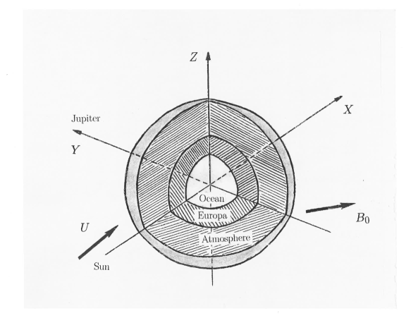
Figure 1.: Europa’s environment and system of coordinates.

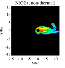
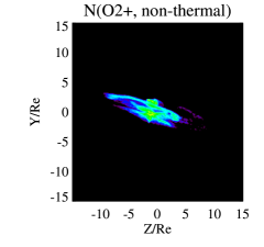
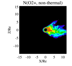
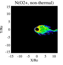
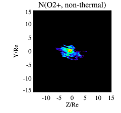
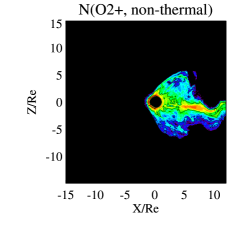
Figure 2.: 2-D cuts of non-thermal pickup ion $O_{2}^{+}$ density profile. Model I, case (a) (top) and case (b) (bottom). $x-y$ cuts (left column) are located at $z=0$, $y-z$ cuts are located at $x/R_{E}=7$, and $x-z$ cuts (right column) are located at $y=0$.

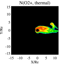
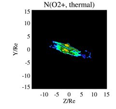
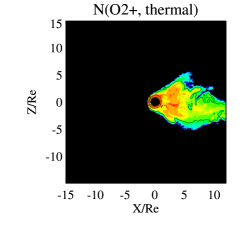
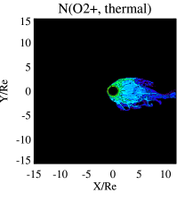
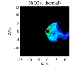
Figure 3.: 2-D cuts of the thermal pickup ion $O_{2}^{+}$ density profile. Model I, case (a) (top) and case (b) (bottom). $x-y$ cuts (left column) are located at $z=0$, $y-z$ cuts are located at $x/R_{E}=7$, and $x-z$ cuts (right column) are located at $y=0$.

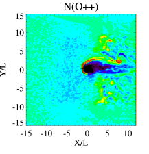
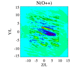
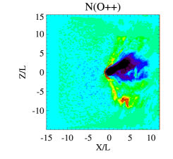
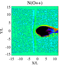
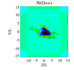
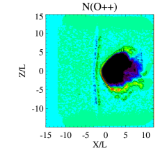
Figure 4.: 2-D cuts of the background $O^{++}$ ion density profiles. Model I, case (a) (top) and case (b) (bottom). $x-y$ cuts (left column) are located at $z=0$, $y-z$ cuts are located at $x/R_{E}=7$, and $x-z$ cuts (right column) are located at $y=0$.

Figure 5.: 1D cuts of the background $O^{++}$ ion density profile. The cuts are located at $y=0$, $z=0$. Model I, case (a) (top) and case (b) (bottom).

Figure 6.: 1D cuts of the background $O^{++}$/$S^{++}$, and pickup non-thermal/thermal ($O_{2}^{+}$) ion densities from simulation. $Y(Re)$ denotes a projection of satellite trajectory onto the $y$ axis. Model I, case (a) (left) and case (b) (right). Bottom - E4 observation of the total ion density (Paterson et al. 1999).

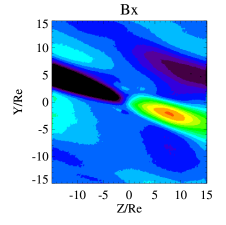
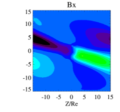
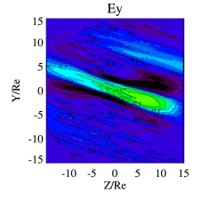
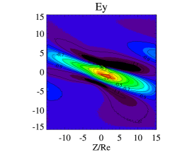
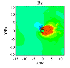
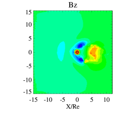
Figure 7.: 2-D cuts of the $B_{x}$, $B_{z}$ magnetic and $E_{y}$ electric field profiles. Model I, case (a) (left) and case (b) (right). $y-z$ cuts (top and middle) are located at $x/R_{E}=7$, and $y-x$ cuts (bottom) are located at $z/R_{E}=0$.

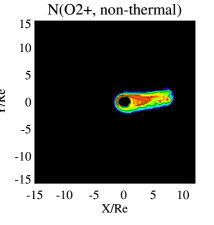
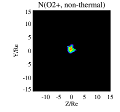
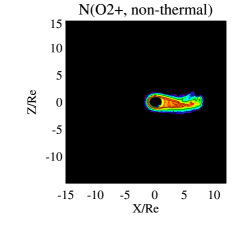
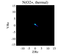
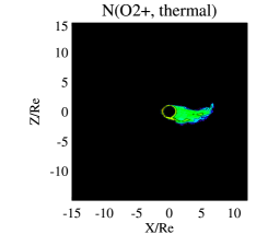
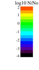
Figure 8.: 2-D cuts of the pickup ion $O_{2}^{+}$ density profile. Non-thermal $O_{2}^{+}$ (top), thermal $O_{2}^{+}$ (bottom). Model II, case (c). $x-y$ cuts (left column) are located at $z=0$, $y-z$ cuts are located at $x/R_{E}=7$, and $x-z$ cuts (right column) are located at $y=0$.

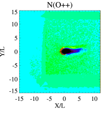
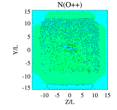
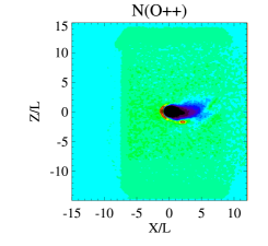
Figure 9.: 2-D cuts of the background $O^{++}$ ion density profiles. Model II, case (c). $x-y$ cuts (left column) are located at $z=0$, $y-z$ cuts are located at $x/R_{E}=7$, and $x-z$ cuts (right column) are located at $y=0$.

Figure 10.: 1D cuts of the background $O^{++}$ ion density profile. The cut is located at $y=0$, $z=0$. Model II, case (c).

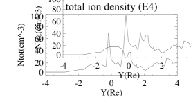
Figure 11.: Background ($S^{++}$, $O^{++}$), non-thermal ($O_{2}^{+}$) and thermal ($O_{2}^{+}$) pickup ion densities from simulation. $Y(Re)$ denotes a projection of the spacecraft position onto the $y$ axis. Model II, case (c). Bottom - E4 observation of the total ion density (Paterson et al. 1999).

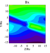
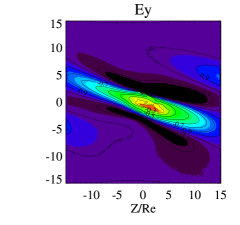
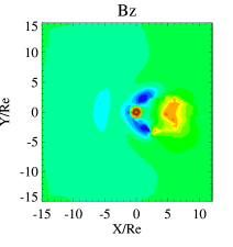
Figure 12.: Model II, case (c). 2-D cuts of the magnetic $B_{x}$ (top), electric $E_{y}$ (top) and magnetic $B_{z}$ (bottom) field profiles. $y-z$ cuts (top) are located at $x/R_{E}=7$, and $y-x$ cuts (bottom) are located at $z/R_{E}=0$.

Figure 13.: Magnetic field component profiles along the E4 trajectory after fitting with inductive dipole magnetic field. Solid line - modeling, (–) denotes dipole field, and (+) is the Jovian magnetic field at the position of Europa. $\circ$ - Galileo’s E4 flyby measurements (Kivelson et al. 1997). $X(Re)$ denotes a projection of the spacecraft position onto the $x$-axis.