Robust Adaptive Beamforming for General-Rank Signal Model with Positive Semi-Definite Constraint via POTDC

Abstract

The robust adaptive beamforming (RAB) problem for general-rank signal model with an additional positive semi-definite constraint is considered. Using the principle of the worst-case performance optimization, such RAB problem leads to a difference-of-convex functions (DC) optimization problem. The existing approaches for solving the resulted non-convex DC problem are based on approximations and find only suboptimal solutions. Here we solve the non-convex DC problem rigorously and give arguments suggesting that the solution is globally optimal. Particularly, we rewrite the problem as the minimization of a one-dimensional optimal value function whose corresponding optimization problem is non-convex. Then, the optimal value function is replaced with another equivalent one, for which the corresponding optimization problem is convex. The new one-dimensional optimal value function is minimized iteratively via polynomial time DC (POTDC) algorithm. We show that our solution satisfies the Karush-Kuhn-Tucker (KKT) optimality conditions and there is a strong evidence that such solution is also globally optimal. Towards this conclusion, we conjecture that the new optimal value function is a convex function. The new RAB method shows superior performance compared to the other state-of-the-art general-rank RAB methods.

I Introduction

It is well known that when the desired signal is present in the training data, the performance of adaptive beamforming methods degrades dramatically in the presence of even a very slight mismatch in the knowledge of the desired signal covariance matrix. The mismatch between the presumed and actual source covariance matrices occurs because of, for example, displacement of antenna elements, time varying environment, imperfections of propagation medium, etc. The main goal of any robust adaptive beamforming (RAB) technique is to provide robustness against any such mismatches.

Most of the RAB methods have been developed for the case of point source signals when the rank of the desired signal covariance matrix is equal to one [1]-[10]. Among the principles used for such RAB methods design are i) the worst-case performance optimization [2]-[5]; ii) probabilistic based performance optimization [7]; and iii) estimation of the actual steering vector of the desired signal [8]-[10]. In many practical applications such as, for example, the incoherently scattered signal source or source with fluctuating (randomly distorted) wavefronts, the rank of the source covariance matrix is higher than one. Although the RAB methods of [1]-[10] provide excellent robustness against any mismatch of the underlying point source assumption, they are not perfectly suited to the case when the rank of the desired signal covariance matrix is higher than one.

The RAB for the general-rank signal model based on the explicit modeling of the error mismatches has been developed in [11] based on the worst-case performance optimization principle. Although the RAB of [11] has a simple closed form solution, it is overly conservative because the worst-case correlation matrix of the desired signal may be negative-definite [12]-[14]. Thus, less conservative approaches have been developed in [12]-[14] by considering an additional positive semi-definite (PSD) constraint to the worst-case signal covariance matrix. The major shortcoming of the RAB methods of [12]-[14] is that they find only a suboptimal solution and there may be a significant gap to the global optimal solution. For example, the RAB of [12] finds a suboptimal solution in an iterative way, but there is no guarantee that such iterative method converges [14]. A closed-form approximate suboptimal solution is proposed in [13], however, this solution may be quite far from the globally optimal one as well. All these shortcomings motivate us to look for new efficient ways to solve the aforementioned non-convex problem globally optimally.

We propose a new method that is based on recasting the original non-convex difference-of-convex functions (DC) programming problem as the minimization of a one dimensional optimal value function. Although the corresponding optimization problem of the newly introduced optimal value function is non-convex, it can be replaced with another equivalent function. The optimization problem that corresponds to such new optimal value function is convex and can be solved efficiently. The new one-dimensional optimal value function is then minimized by the means of the newly designed polynomial time DC (POTDC) algorithm (see also [16], [17]). We prove that the point found by the POTDC algorithm for RAB for general-rank signal model with positive semi-definite constraint is a Karush-Kuhn-Tucker (KKT) optimal point. Moreover, we prove a number of results that lead us to the equivalence between the claim of global optimality for the POTDC algorithm as applied to the problem under consideration and the convexity of the newly obtained one-dimensional optimal value function. The latter convexity of the newly obtained one-dimensional optimal value function can be checked numerically by using the convexity on lines property of convex functions. The fact that enables such numerical check is that the argument of such optimal value function is proved to take values only in a closed interval. In addition, we also develop tight lower-bound for such optimal value function that is used in the simulations for further confirming global optimality of the POTDC method.

The rest of the paper is organized as follows. System model and preliminaries are given in Section II, while the problem is formulated in Section III. The new proposed method is developed in Section IV followed by the simulation results in Section V. Finally, Section VI presents our conclusions. This paper is reproducible research and the software needed to generate the simulation results will be provided to the IEEE Xplore together with the paper upon its acceptance.

II System Model and Preliminaries

The narrowband signal received by a linear antenna array with $M$ omni-directional antenna elements at the time instant $k$ can be expressed as

$$\mathbf{x}(k)=\mathbf{s}(k)+\mathbf{i}(k)+\mathbf{n}(k)$$ (1)

where $\mathbf{s}(k)$, $\mathbf{i}(k)$, and $\mathbf{n}(k)$ are the statistically independent $M\times 1$ vectors of the desired signal, interferences, and noise, respectively. The beamformer output at the time instant $k$ is given as

$$y(k)=\mathbf{w}^{H}\mathbf{x}(k)\vspace{-1mm}$$ (2)

where $\mathbf{w}$ is the $M\times 1$ complex beamforming vector of the antenna array and $(\cdot)^{H}$ stands for the Hermitian transpose. The beamforming problem is formulated as finding the beamforming vector $\mathbf{w}$ which maximizes the beamformer output signal-to-interference-plus-noise ratio (SINR) given as

$$\mathrm{SINR}=\frac{\mathbf{w}^{H}{\mathbf{R}_{\rm s}}\mathbf{w}}{\mathbf{w}^{H}{\mathbf{R}_{\rm i+n}}\mathbf{w}}$$ (3)

where $\mathbf{R}_{\rm s}\triangleq E\{\mathbf{s}(k)\mathbf{s}(k)^{H}\}$ and $\mathbf{R}_{\rm i+n}\triangleq E\{(\mathbf{i}(k)+\mathbf{n}(k))(\mathbf{i}(k)+\mathbf{n}(k))^{H}\}$ are the desired signal and interference-plus-noise covariance matrices, respectively, and $E\{\cdot\}$ stands for the statistical expectation.

Depending on the nature of the desired signal source, its corresponding covariance matrix can be of an arbitrary rank, i.e., $1\leq{\rm rank}\{\mathbf{R}_{\rm s}\}\leq M$, where ${\rm rank}\{\cdot\}$ denotes the rank operator. Indeed, in many practical applications, for example, in the scenarios with incoherently scattered signal sources or signals with randomly fluctuating wavefronts, the rank of the desired signal covariance matrix $\mathbf{R}_{\rm s}$ is greater than one [11]. The only particular case in which, the rank of $\mathbf{R}_{\rm s}$ is equal to one is the case of the point source.

The interference-plus-noise covariance matrix $\mathbf{R}_{\rm i+n}$ is typically unavailable in practice and it is substituted by the data sample covariance matrix

$$\hat{\mathbf{R}}=\frac{1}{K}\sum_{i=1}^{K}\mathbf{x}(i)\mathbf{x}^{H}(i)$$ (4)

where $K$ is number of the training data samples. The problem of maximizing the SINR (3) (here we always use sample matrix estimate $\hat{\mathbf{R}}$ instead of $\mathbf{R}_{\rm i+n}$) is known as minimum variance distortionless response (MVDR) beamforming and can be mathematically formulated as

$$\min\limits_{{\bf w}}{\bf w}^{H}\hat{\mathbf{R}}{\bf w}\quad{\rm s.t.}\quad{\bf w}^{H}\mathbf{R}_{\rm s}{\bf w}=1.$$ (5)

The solution to the MVDR beamforming problem (5) can be found as [1]

$${\mathbf{w}}_{\rm SMI-MVDR}={\boldsymbol{\cal P}}\{\hat{\mathbf{R}}^{-1}\mathbf{R}_{\rm s}\}$$ (6)

which is known as the sample matrix inversion (SMI) MVDR beamformer for general-rank signal model. Here ${\boldsymbol{\cal P}}\{\cdot\}$ stands for the principal eigenvector operator.

In practice, the actual desired signal covariance matrix $\mathbf{R}_{\rm s}$ is usually unknown and only its presumed value is available. The actual source correlation matrix can be modeled as $\mathbf{R}_{\rm s}=\tilde{\mathbf{R}}_{\rm s}+\boldsymbol{\Delta}_{1}$, where $\boldsymbol{\Delta}_{1}$ and $\tilde{\mathbf{R}}_{\rm s}$ denote an unknown mismatch and the presumed correlation matrices, respectively. It is well known that the MVDR beamformer is very sensitive to such mismatches [11]. RABs also address the situation when the sample estimate of the data covariance matrix (4) is inaccurate (for example, because of small sample size) and $\mathbf{R}=\hat{\mathbf{R}}+\mathbf{\Delta}_{2}$, where $\mathbf{\Delta}_{2}$ is an unknown mismatch matrix to the data sample covariance matrix. In order to provide robustness against the norm-bounded mismatches $\|\mathbf{\Delta}_{1}\|\leq\epsilon$ and $\|\mathbf{\Delta}_{2}\|\leq\gamma$ (here $\|\cdot\|$ denotes the Frobenius norm of a matrix), the RAB of [11] uses the worst-case performance optimization principle of [2] and finds the solution as

$$\mathbf{w}={\boldsymbol{\cal P}}\{(\hat{\mathbf{R}}+\gamma\mathbf{I})^{-1}(\tilde{\mathbf{R}}_{\rm s}-\epsilon\mathbf{I})\}.$$ (7)

Although the RAB of [11] has a simple closed-form solution (7), it is overly conservative because the constraint that the matrix $\tilde{\mathbf{R}}_{\rm s}+\boldsymbol{\Delta}_{1}$ has to be positive semi-definite (PSD) is not considered [12]. For example, the worst-case desired signal covariance matrix $\tilde{\mathbf{R}}_{\rm s}-\epsilon\mathbf{I}$ in (7) can be indefinite or negative definite if $\tilde{\mathbf{R}}_{\rm s}$ is rank deficient. Indeed, in the case of incoherently scattered source, $\tilde{\mathbf{R}}_{\rm s}$ has the following form $\tilde{\mathbf{R}}_{\rm s}=\sigma_{\rm s}^{2}\int_{-\pi/2}^{\pi/2}\zeta(\theta)\mathbf{a}(\theta)\mathbf{a}^{H}(\theta)d\theta$, where $\zeta(\theta)$ denotes the normalized angular power density, $\sigma_{\rm s}^{2}$ is the desired signal power, and $\mathbf{a}(\theta)$ is the steering vector towards direction $\theta$. For a uniform angular power density on the angular bandwidth $\Phi$, the approximate numerical rank of $\tilde{\mathbf{R}}_{\rm s}$ is equal to $(\Phi/\pi)\cdot M$ [18]. This leads to a rank deficient matrix $\tilde{\mathbf{R}}_{\rm s}$ if the angular power density does not cover all the directions. Therefore, the worst-case covariance matrix $\tilde{\mathbf{R}}_{\rm s}-\epsilon\mathbf{I}$ is indefinite or negative definite. Note that the worst-case data sample covariance matrix $\hat{\mathbf{R}}+\gamma\mathbf{I}$ is always positive definite.

III Problem Formulation

Decomposing $\mathbf{R}_{\rm s}$ as $\mathbf{R}_{\rm s}=\mathbf{Q}^{H}\mathbf{Q}$, the RAB problem for a norm bounded-mismatch $\|\mathbf{\Delta}\|\leq\eta$ to the matrix $\mathbf{Q}$ is given as [12]

$$\min\limits_{\mathbf{w}} \max_{\|\mathbf{\Delta}_{2}\|\leq\gamma}\mathbf{w}^{H}(\hat{\mathbf{R}}+\mathbf{\Delta}_{2})\mathbf{w}$$ (8)

$${\rm s.t.} \min_{\|\mathbf{\Delta}\|\leq\eta}\mathbf{w}^{H}(\mathbf{Q}\!+\!\mathbf{\Delta})^{H}(\mathbf{Q}\!+\!\mathbf{\Delta})\mathbf{w}\!\geq\!1.$$

For every $\mathbf{\Delta}$ in the optimization problem (8) whose norm is less than or equal to $\eta$, the expression $\mathbf{w}^{H}(\mathbf{Q}\!+\!\mathbf{\Delta})^{H}(\mathbf{Q}\!+\!\mathbf{\Delta})\mathbf{w}\!\geq\!1$ represents a non-convex quadratic constraint with respect to $\mathbf{w}$. Because there exists infinite number of mismatches $\mathbf{\Delta}$, there also exists infinite number of such non-convex quadratic constraints. By finding the minimum possible value of the quadratic term $\mathbf{w}^{H}(\mathbf{Q}\!+\!\mathbf{\Delta})^{H}(\mathbf{Q}\!+\!\mathbf{\Delta})\mathbf{w}$ with respect to $\mathbf{\Delta}$ for a fixed $\mathbf{w}$, the infinite number of such non-convex quadratic constraints can be replaced with a single constraint. For this goal, we consider the following optimization problem

$$\min\limits_{\mathbf{\Delta}} \mathbf{w}^{H}(\mathbf{Q}\!+\!\mathbf{\Delta})^{H}(\mathbf{Q}\!+\!\mathbf{\Delta})\mathbf{w}$$

$${\rm s.t.} \|\mathbf{\Delta}\|^{2}\leq\eta^{2}$$ (9)

where $\mathbf{\Delta}$ is a Hermitian matrix. This problem is convex and its optimal value can be expressed as a function of $\mathbf{w}$ as given by the following lemma.

Lemma 1: The optimal value of the optimization problem (9) as a function of $\mathbf{w}$ is equal to

$$\min\limits_{\|\mathbf{\Delta}\|^{2}\leq\eta^{2}}\mathbf{w}^{H}(\mathbf{Q}\!+\!\mathbf{\Delta})^{H}(\mathbf{Q}\!+\!\mathbf{\Delta})\mathbf{w}$$

$$=\left\{\begin{array}[]{ll}(\|\mathbf{Q}\mathbf{w}\|-\eta\|\ \!\mathbf{w}\|)^{2},&\quad\|\mathbf{Q}\mathbf{w}\|\geq\eta\|\mathbf{w}\|\\ 0,&\quad\ \mbox{otherwise.}\end{array}\right.$$ (12)

Proof:

See Appendix, Subsection VII-A. ∎

The maximum of the quadratic term $\mathbf{w}^{H}(\hat{\mathbf{R}}+\mathbf{\Delta}_{2})\mathbf{w}$ with respect to $\mathbf{\Delta}_{2}$, $\|\mathbf{\Delta}_{2}\|\leq\gamma$ that appears in the the objective of the problem (8) can be easily derived as $\mathbf{w}^{H}(\hat{\mathbf{R}}+\gamma\mathbf{I})\mathbf{w}$. It is obvious from (12) that the desired signal can be totally removed from the beamformer output if $\|\mathbf{Q}\mathbf{w}\|<\eta\|\mathbf{w}\|$. Based on the later fact, $\|\mathbf{Q}\mathbf{w}\|-\eta\|\mathbf{w}\|$ should be greater than or equal to zero. For any such $\mathbf{w}$, the new constraint in the optimization problem (9) can be expressed as $\|\mathbf{Q}\mathbf{w}\|-\eta\|\ \mathbf{w}\|\geq 1$. Since $\|\mathbf{Q}\mathbf{w}\|-\eta\|\ \!\mathbf{w}\|\geq 1$ also implies that $\|\mathbf{Q}\mathbf{w}\|-\eta\|\mathbf{w}\|\geq 0$, the RAB problem (8) can be equivalently rewritten as

$$\min\limits_{\mathbf{w}} \,\mathbf{w}^{H}(\hat{\mathbf{R}}+\gamma\mathbf{I})\mathbf{w}\quad$$ (13)

$${\rm s.t.} \quad\|\mathbf{Q}\mathbf{w}\|-\eta\|\ \!\!\mathbf{w}\|\geq 1\;.$$

Due to the non-convex DC constraint, (13) is non-convex DC programming problem [16], [17]. DC optimization problems are believed to be NP-hard in general [19], [20]. There is a number of methods that can be applied to DC problems of type (13) in the literature. Among these methods are the generalized polyblock algorithm, the extended general power iterative (GPI) algorithm [21], DC iteration-based method [22], etc. However, the existing methods do not guarantee to find the solution of (13), i.e., to converge to the global optimum of (13) in polynomial time. This means that the problem (13) is NP-hard. The best what is possible to show, for example, for the DC iteration-based method is that it can find a KKT optimal point. The overall computational complexity of the DC iteration-based method can be, however, quite high because the number of iterations required to converge grows dramatically with the dimension of the problem.

Recently, the problem (13) has also been suboptimally solved using an iterative semi-definite relaxation (SDR)-based algorithm in [12] which also does not result in the globally optimal solution and for which the convergence even to a KKT optimal point is not guaranteed. A closed-form suboptimal solution for the aforementioned non-convex DC problem has been also derived in [13]. Despite its computational simplicity, the performance of the method of [13] may be far from the global optimum and even the KKT optimal point. Another iterative algorithm has been proposed in [14], but it modifies the problem (13) and solves the modified problem instead which again gives no guarantees for finding the globally optimal solution of the original problem (13). In what follows, we develop a new polynomial time algorithm for addressing the DC programming problems of type (13), prove that it finds at least a KKT optimal point of the problem, and attempt to prove that it actually solves the problem.

IV New Proposed Method

In this section, we aim at solving the problem (13) in a rigorous way, i.e., without using any type of approximations. For this goal, we design a POTDC-type algorithm (see also [16], [17]) that can be used for solving a class of DC programming problems in polynomial time. More specifically, the POTDC algorithm can be efficiently used for DC programming problems whose non-convex parts are functions of only one variable. By introducing the auxiliary optimization variable $\alpha\geq 1$ and setting $\|\mathbf{Q}\mathbf{w}\|=\sqrt{\alpha}$, the problem (13) can be equivalently rewritten as

$$\min_{\mathbf{w},\alpha} \,\mathbf{w}^{H}(\hat{\mathbf{R}}+\gamma\mathbf{I})\mathbf{w}\quad$$

$${\rm s.t.} \mathbf{w}^{H}\mathbf{Q}^{H}\mathbf{Q}\mathbf{w}=\alpha$$ (14)

$$\mathbf{w}^{H}\mathbf{w}\leq\frac{(\sqrt{\alpha}-1)^{2}}{\eta^{2}},\quad\alpha\geq 1.$$

Note that $\alpha$ is restricted to be greater than or equal to one because $\|\mathbf{Q}\mathbf{w}\|$ is greater than or equal to one due to the constraint of the problem (13). For future needs, we find the set of all $\alpha$’s for which the optimization problem (14) is feasible. Let us define the following set for a fixed value of $\alpha\geq 1$,

$$S(\alpha)=\{\mathbf{w}\ |\ \mathbf{w}^{H}\mathbf{w}\leq(\sqrt{\alpha}-1)^{2}/\eta^{2}\}.$$ (15)

It is trivial that for every $\mathbf{w}\in S(\alpha)$, the quadratic term $\mathbf{w}^{H}\mathbf{Q}^{H}\mathbf{Q}\mathbf{w}$ is non-negative as $\mathbf{Q}^{H}\mathbf{Q}$ is a positive semi-definite matrix. Using the minimax theorem [23], it can be easily verified that the maximum value of the quadratic term $\mathbf{w}^{H}\mathbf{Q}^{H}\mathbf{Q}\mathbf{w}$ over $\mathbf{w}\in S(\alpha)$ is equal to $\left((\sqrt{\alpha}-1)^{2}/\eta^{2}\right)\cdot\lambda_{\rm max}\{\mathbf{Q}^{H}\mathbf{Q}\}$ and this value is achieved by

$$\mathbf{w}_{\alpha}=\frac{\sqrt{\alpha}-1}{\eta}{\boldsymbol{\cal P}}\{\mathbf{Q}^{H}\mathbf{Q}\}\ \in\ S(\alpha).$$ (16)

Here $\lambda_{\rm max}\{\cdot\}$ stands for the largest eigenvalue operator. Due to the fact that for any $0\leq\beta\leq 1$, the scaled vector $\beta\mathbf{w}_{\alpha}$ lies inside the set $S(\alpha)$ (15), the quadratic term $\mathbf{w}^{H}\mathbf{Q}^{H}\mathbf{Q}\mathbf{w}$ can take values only in the interval $[0,\left((\sqrt{\alpha}-1)^{2}/\eta^{2}\right)\cdot\lambda_{\rm max}\{\mathbf{Q}^{H}\mathbf{Q}\}]$ over $\mathbf{w}\in S(\alpha)$.

Considering the later fact and also the optimization problem (14), it can be concluded that $\alpha$ is feasible if and only if $\alpha\in[0,\left((\sqrt{\alpha}-1)^{2}/\eta^{2}\right)\cdot\lambda_{\rm max}\{\mathbf{Q}^{H}\mathbf{Q}\}]$ which implies that

$$\frac{(\sqrt{\alpha}-1)^{2}}{\eta^{2}}\cdot\lambda_{\rm max}\{\mathbf{Q}^{H}\mathbf{Q}\}\geq\alpha$$ (17)

or, equivalently, that

$$\frac{(\sqrt{\alpha}-1)^{2}}{\alpha}\geq\frac{\eta^{2}}{\lambda_{\rm max}\{\mathbf{Q}^{H}\mathbf{Q}\}}.$$ (18)

The function $(\sqrt{\alpha}-1)^{2}/\alpha$ is strictly increasing and it is also less than or equal to one for $\alpha\geq 1$. Therefore, it can be immediately found that the problem (14) is infeasible for any $\alpha\geq 1$ if $\lambda_{\rm max}\{\mathbf{Q}^{H}\mathbf{Q}\}\leq\eta^{2}$. Thus, hereafter, it is assumed that $\lambda_{\rm max}\{\mathbf{Q}^{H}\mathbf{Q}\}>\eta^{2}$. Moreover, using (18) and the fact that the function $(\sqrt{\alpha}-1)^{2}/\alpha$ is strictly increasing, it can be found that the feasible set of the problem (14) corresponds to

$$\alpha\geq\frac{1}{\left(1-\frac{\eta}{\sqrt{\lambda_{\rm max}\{\mathbf{Q}^{H}\mathbf{Q}\}}}\right)^{2}}\geq 1.$$ (19)

As we will see in the following sections, for developing the POTDC algorithm for the problem (14), an upper-bound for the optimal value of $\alpha$ in (14) is needed. Such upper-bound is obtained in terms of the following lemma.

Lemma 2: The optimal value of the optimization variable $\alpha$ in the problem (14) is upper-bounded by $\lambda_{\rm max}\left\{(\hat{\mathbf{R}}+\gamma\mathbf{I})^{-1}\mathbf{Q}^{H}\mathbf{Q}\right\}\cdot\mathbf{w}_{0}^{H}(\hat{\mathbf{R}}+\gamma\mathbf{I})\mathbf{w}_{0}$, where $\mathbf{w}_{0}$ is any arbitrary feasible point of the problem (14).

Proof:

See Appendix, Subsection VII-B. ∎

Using Lemma 2, the problem (14) can be equivalently stated as

$$\min\limits_{\theta_{1}\leq\alpha\leq\theta_{2}} \overbrace{\min\limits_{\mathbf{w}}\mathbf{w}^{H}(\hat{\mathbf{R}}+\gamma\mathbf{I})\mathbf{w}}^{\text{Inner Problem}}$$ (20)

$${\rm s.t.} \mathbf{w}^{H}\mathbf{Q}^{H}\mathbf{Q}\mathbf{w}\!=\alpha,$$

$$\mathbf{w}^{H}\mathbf{w}\!\leq\!\frac{(\sqrt{\alpha}\!-\!1)^{2}}{\eta^{2}}$$

where

$$\theta_{1}=\frac{1}{{\left(1-\frac{\eta}{\sqrt{\lambda_{\rm max}\{\mathbf{Q}^{H}\mathbf{Q}\}}}\ \right)^{2}}}$$ (21)

and

$$\theta_{2}=\lambda_{\rm max}\left\{(\hat{\mathbf{R}}+\gamma\mathbf{I})^{-1}\mathbf{Q}^{H}\mathbf{Q}\right\}\mathbf{w}_{0}^{H}(\hat{\mathbf{R}}+\gamma\mathbf{I})\mathbf{w}_{0}.$$ (22)

It is easy to verify that $\theta_{2}\geq\theta_{1}$. For a fixed value of $\alpha$, the inner optimization problem in (20) is non-convex with respect to $\mathbf{w}$. Based on the inner optimization problem in (20) when $\alpha$ is fixed, we define the following optimal value function

$$h(\alpha)\triangleq\Big{\{}\min\limits_{\mathbf{w}}\mathbf{w}^{H}(\hat{\mathbf{R}}\!+\!\gamma\mathbf{I})\mathbf{w}\ |\ \mathbf{w}^{H}\mathbf{Q}^{H}\mathbf{Q}\mathbf{w}\!=\alpha,$$

$$\ \mathbf{w}^{H}\mathbf{w}\!\leq\!\frac{(\sqrt{\alpha}\!-\!1)^{2}}{\eta^{2}}\Big{\}},\quad\theta_{1}\leq\alpha\leq\theta_{2}.$$ (23)

Using the optimal value function (23), the problem (20) can be equivalently expressed as

$$\min\limits_{\alpha} h(\alpha)\quad{\rm s.t.}\quad\theta_{1}\leq\alpha\leq\theta_{2}.$$ (24)

The corresponding optimization problem of $h(\alpha)$ for a fixed value of $\alpha$ is non-convex. In what follows, we aim at replacing $h(\alpha)$ with an equivalent optimal value function whose corresponding optimization problem is convex.

Introducing the matrix $\mathbf{W}\triangleq\mathbf{w}\mathbf{w}^{H}$ and using the fact that for any arbitrary matrix $\mathbf{A}$, $\mathbf{w}^{H}\mathbf{A}\mathbf{w}={\rm tr}\{\mathbf{A}\mathbf{w}\mathbf{w}^{H}\}$ (here ${\rm tr}\{\cdot\}$ stands for the trace of a matrix), the function (23) can be equivalently recast as

$$\!\!\!\!\!\!\!\!\!\!h(\alpha)=\Big{\{}\min\limits_{\mathbf{W}}{\rm tr}\big{\{}(\hat{\mathbf{R}}+\gamma\mathbf{I})\mathbf{W}\big{\}}\ |\ {\rm tr}\{\mathbf{Q}^{H}\mathbf{Q}\mathbf{W}\}=\alpha,$$

$${\rm tr}\{\mathbf{W}\}\!\leq\!\frac{(\sqrt{\alpha}\!-\!1)^{2}}{\eta^{2}},\ \mathbf{W}\succeq\mathbf{0},\ {\rm rank}\{\mathbf{W}\}=1\Big{\}},$$

$$\quad\quad\theta_{1}\leq\alpha\leq\theta_{2}$$ (25)

Dropping the rank-one constraint in the corresponding optimization problem of $h(\alpha)$ for a fixed value of $\alpha$, $(\theta_{1}\leq\alpha\leq\theta_{2})$, a new optimal value function denoted as $k(\alpha)$ can be defined as

$$k(\alpha) \triangleq \Big{\{}\min\limits_{\mathbf{W}}{\rm tr}\big{\{}(\hat{\mathbf{R}}+\gamma\mathbf{I})\mathbf{W}\big{\}}\ |\ {\rm tr}\{\mathbf{Q}^{H}\mathbf{Q}\mathbf{W}\}=\alpha,$$ (26)

$$\ {\rm tr}\{\mathbf{W}\}\!\leq\!\frac{(\sqrt{\alpha}\!-\!1)^{2}}{\eta^{2}},\ \mathbf{W}\succeq\mathbf{0}\Big{\}},$$

$$\theta_{1}\leq\alpha\leq\theta_{2}.$$

For brevity, we will refer to the optimization problems that correspond to the optimal value functions $h(\alpha)$ and $k(\alpha)$ when $\alpha$ is fixed, as the optimization problems of $h(\alpha)$ and $k(\alpha)$, respectively. Note also that compared to the optimization problem of $h(\alpha)$, the optimization problem of $k(\alpha)$ is convex. More importantly, the following lemma establishes the equivalence between the optimal value functions $h(\alpha)$ and $k(\alpha)$.

Lemma 3: The optimal value functions $h(\alpha)$ and $k(\alpha)$ are equivalent, i.e., $h(\alpha)=k(\alpha)$ for any $\alpha\in[\theta_{1},\theta_{2}]$. Furthermore, based on the optimal solution of the optimization problem of $k(\alpha)$ when $\alpha$ is fixed, the optimal solution of the optimization problem of $h(\alpha)$ can be constructed.

Proof:

See Appendix, Subsection VII-C. ∎

Based on Lemma 3, the original problem (24) can be expressed as

$$\min\limits_{\alpha} k(\alpha)\quad{\rm s.t.}\quad\theta_{1}\leq\alpha\leq\theta_{2}$$ (27)

It is noteworthy to mention that based on the optimal solution of (27) denoted as $\alpha_{\rm opt}$, we can easily obtain the optimal solution of the original problem (24) or, equivalently, the optimal solution of the problem (20). Specifically, since the optimal value functions $h(\alpha)$ and $k(\alpha)$ are equivalent, $\alpha_{\rm opt}$ is also the optimal solution of the problem (24) and, thus, also the problem (20). Moreover, the optimization problem of $k(\alpha_{\rm opt})$ is convex and can be easily solved. In addition, using the results in Lemma 3, based on the optimal solution of the optimization problem of $k(\alpha_{\rm opt})$, the optimal solution of the optimization problem of $h(\alpha_{\rm opt})$ can be constructed. Therefore, in the rest of the paper, we concentrate on the problem (27).

Since for every fixed value of $\alpha$, the corresponding optimization problem of $k(\alpha)$ is a convex semi-definite programming (SDP) problem, one possible approach for solving (27) is based on exhaustive search over $\alpha$. In other words, $\alpha$ can be found by using an exhaustive search over a fine grid on the interval of $[\theta_{1},\theta_{2}]$. Although this search method is inefficient, it can be used as a benchmark.

Using the definition of the optimal value function $k(\alpha)$, the problem (27) can be equivalently expressed as

$$\min\limits_{\mathbf{W},\alpha} \!\!\!\!\!{\rm tr}\left\{\mathbf{(\hat{\mathbf{R}}\!+\!\gamma\mathbf{I})}\mathbf{W}\right\}\quad$$ (28)

$${\rm s.t.} {\rm tr}\{\mathbf{Q}^{H}\mathbf{Q}\mathbf{W}\}\!=\!\alpha$$

$${\eta^{2}}{\rm tr}\{\mathbf{W}\}\!\leq\!(\sqrt{\alpha}\!-\!1)^{2}$$

$$\mathbf{W}\succeq 0,\ \theta_{1}\leq\alpha\leq\theta_{2}.$$

Note that replacing $h(\alpha)$ by $k(\alpha)$ results in a much simpler problem. Indeed, compared to the original problem (20), in which the first constraint is non-convex, the corresponding first constraint of (28) is convex. All the constraints and the objective function of the problem (28) are convex except for the constraint ${\rm tr}\{\mathbf{W}\}\leq(\sqrt{\alpha}-1)^{2}/\eta^{2}$ which is non-convex only in a single variable $\alpha$ and which makes the problem (28) non-convex overall. This single non-convex constraint can be rewritten equivalently as $\eta^{2}{\rm tr}\{\mathbf{W}\}-(\alpha+1)+2\sqrt{\alpha}\leq 0$ where all the terms are linear with respect to $\mathbf{W}$ and $\alpha$ except for the concave term of $\sqrt{\alpha}$. The latter constraint can be handled iteratively by building a POTDC-type algorithm (see also [16], [17]) based on the iterative linear approximation of the non-convex term $\sqrt{\alpha}$ around suitably selected points. It is interesting to mention that this iterative linear approximation can be also interpreted in terms of DC iteration over a single non-convex term $\sqrt{\alpha}$. The fact that iterations are needed only over a single variable helps to reduce dramatically the number of iterations of the algorithm and allows for very simple interpretations shown below.

IV-A Iterative POTDC Algorithm

Let us consider the optimization problem (28) and replace the term $\sqrt{\alpha}$ by its linear approximation around $\alpha_{c}$, i.e., $\sqrt{\alpha}\approx\sqrt{\alpha_{c}}+(\alpha-\alpha_{c})/(2\sqrt{\alpha_{c}})$. It leads to the following SDP problem

$$\min\limits_{\mathbf{W},\alpha} \!\!\!\!{\rm tr}\left\{(\hat{\mathbf{R}}+\gamma\mathbf{I})\mathbf{W}\right\}\quad$$ (29)

$${\rm s.t.} \!\!\!\!{\rm tr}\{\mathbf{Q}^{H}\mathbf{Q}\mathbf{W}\}=\alpha$$

$$\!\!\!\!\eta^{2}{\rm tr}\{\mathbf{W}\!\}\!+\!(\sqrt{\alpha_{c}}\!-\!1)\!+\!\alpha\left(\frac{1}{\sqrt{\alpha_{c}}}\!-\!1\!\right)\leq\!0$$

$$\!\!\!\!\mathbf{W}\succeq 0,\ \ \theta_{1}\leq\alpha\leq\theta_{2}.$$

To understand the POTDC algorithm intuitively and also to see how the linearization points are selected in different iterations, let us define the following optimal value function based on the optimization problem (29)

$$l(\alpha,\alpha_{c})\triangleq\!\!\!\!\! \Big{\{} \!\!\!\!\!\min\limits_{\mathbf{W}}{\rm tr}\big{\{}(\hat{\mathbf{R}}+\gamma\mathbf{I})\mathbf{W}\big{\}}\ |\ {\rm tr}\{\mathbf{Q}^{H}\mathbf{Q}\mathbf{W}\}=\alpha,$$ (30)

$$\eta^{2}{\rm tr}\{\mathbf{W}\!\}\!+\!(\sqrt{\alpha_{c}}\!-\!1)\!+\!\alpha\left(\frac{1}{\sqrt{\alpha_{c}}}\!-\!1\!\right)\leq\!0,$$

$$\mathbf{W}\succeq\mathbf{0}\Big{\}},\ \ \ \ \theta_{1}\leq\alpha\leq\theta_{2}.$$

where $\alpha_{c}$ in $l(\alpha,\alpha_{c})$ denotes the linearization point. The optimal value function $l(\alpha,\alpha_{c})$ can be also obtained through $k(\alpha)$ in (26) by replacing the term $\sqrt{\alpha}$ in $\eta^{2}{\rm tr}\{\mathbf{W}\}-(\alpha+1)+2\sqrt{\alpha}\leq 0$ with its linear approximation around $\alpha_{c}$. Since $\sqrt{\alpha}$ and its linear approximation have the same values at $\alpha_{c}$, $l(\alpha,\alpha_{c})$ and $k(\alpha)$ take the same values at this point. The following lemma establishes the relationship between the optimal value functions $k(\alpha)$ and $l(\alpha,\alpha_{c})$.

Lemma 4: $l(\alpha,\alpha_{c})$ is a convex upper-bound of $k(\alpha)$ for any arbitrary $\alpha_{c}\in[\theta_{1},\theta_{2}]$, i.e., $l(\alpha,\alpha_{c})\geq k(\alpha)$, $\forall\alpha\in[\theta_{1},\theta_{2}]$ and $l(\alpha,\alpha_{c})$ is convex with respect to $\alpha$. Furthermore, the values of the optimal value functions $k(\alpha)$ and $l(\alpha,\alpha_{c})$ as well as their right and left derivatives are equal at this point. In other words, under the condition that $k(\alpha)$ is differentiable at $\alpha_{c}$, $l(\alpha,\alpha_{c})$ is tangent to $k(\alpha)$ at this point.

Proof:

See Appendix, Subsection VII-D. ∎

In what follows, for the sake of clarity of the explanations, it is assumed that the function $k(\alpha)$ is differentiable over the interval of $(\theta_{1},\theta_{2})$, however, this property is not generally required as we will see later. Let us consider an arbitrary point, denoted as $\alpha_{0}$, $\alpha_{0}\in(\theta_{1},\theta_{2})$ as the initial linearization point, i.e., $\alpha_{c}=\alpha_{0}$. Based on Lemma 4, $l(\alpha,\alpha_{0})$ is a convex function with respect to $\alpha$ which is tangent to $k(\alpha)$ at the linearization point $\alpha=\alpha_{0}$, and it is also an upper-bound to $k(\alpha)$. Let $\alpha_{1}$ denote the global minimizer of $l(\alpha,\alpha_{0})$ that can be easily obtained due to the convexity of $l(\alpha,\alpha_{0})$ with polynomial time complexity.

Since $l(\alpha,\alpha_{0})$ is tangent to $k(\alpha)$ at $\alpha=\alpha_{0}$ and it is also an upper-bound for $k(\alpha)$, it can be concluded that $\alpha_{1}$ is a decent point for $k(\alpha)$, i.e., $k(\alpha_{1})\leq k(\alpha_{0})$ as it is shown in Fig.1. Specifically, the fact that $l(\alpha,\alpha_{0})$ is tangent to $k(\alpha)$ at $\alpha=\alpha_{0}$ and $\alpha_{1}$ is the global minimizer of $l(\alpha,\alpha_{0})$ implies that

$$l(\alpha_{1},\alpha_{0})\leq l(\alpha_{0},\alpha_{0})=k(\alpha_{0}).$$ (31)

Furthermore, since $l(\alpha,\alpha_{0})$ is an upper-bound for $k(\alpha)$, it can be found that $k(\alpha_{1})\leq l(\alpha_{1},\alpha_{0})$. Due to the later fact and also the equation (31), it is concluded that $k(\alpha_{1})\leq k(\alpha_{0})$.

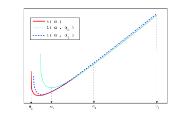
Figure 1: Iterative method for minimizing the optimal value function $k(\alpha)$. The convex optimal value function $l(\alpha,\alpha_{0})$ is an upper bound to $k(\alpha)$ which is tangent to it at $\alpha=\alpha_{0}$, and its minimum is denoted as $\alpha_{1}$. The point $\alpha_{1}$ is used to establish another convex upper-bound function denoted as $l(\alpha,\alpha_{1})$ and this proces continutes.

Choosing $\alpha_{1}$ as the linearzation point in the second iteration, and finding the global minimizer of $l(\alpha,\alpha_{1})$ over the interval $[\theta_{1},\theta_{2}]$ denoted as $\alpha_{2}$, another decent point can be obtained, i.e., $k(\alpha_{2})\leq k(\alpha_{1})$. This process can be continued until convergence.

Then the proposed iterative decent method can be described as shown in Algorithm 1. The following lemma about the convergence of Algorithm 1 and the optimality of the solution obtained by this algorithm is in order. Note that this lemma makes no assumptions about the differentiability of the optimal value function $k(\alpha)$.

Lemma 5: The following statements regarding Algorithm 1 are true:

i)

The optimal value of the optimization problem in Algorithm 1 is non-increasing over iterations, i.e.,

$$\!\!\!\!\!\!\!\!\!\!\!\!{\rm tr}\!\left\{(\hat{\mathbf{R}}+\gamma\mathbf{I})\mathbf{W}_{opt,i+1}\right\}\leq{\rm tr}\!\left\{(\hat{\mathbf{R}}+\gamma\mathbf{I})\mathbf{W}_{opt,i}\right\},$$

$$\ i\geq 1.$$

ii)

Algorithm 1 converges.

iii)

Algorithm 1 converges to a KKT solution, i.e., a solution which satisfies the KKT optimality conditions.

Proof:

See Appendix, Subsection VII-E. ∎

Algorithm 1 The iterative POTDC algorithm

0:  An arbitrary $\alpha_{c}\in[\theta_{1},\theta_{2}]$,      the termination threshold $\zeta$,      set $i$ equal to 1.

  repeat

     Solve the following optimization problem using $\alpha_{c}$ to obtain $\mathbf{W}_{opt}$ and $\alpha_{opt}$

$$\min\limits_{\mathbf{W},\alpha} \!\!\!\!{\rm tr}\left\{(\hat{\mathbf{R}}+\gamma\mathbf{I})\mathbf{W}\right\}\quad$$

$${\rm s.t.} \!\!\!\!{\rm tr}\{\mathbf{Q}^{H}\mathbf{Q}\mathbf{W}\}=\alpha$$

$$\!\!\!\!\eta^{2}{\rm tr}\{\mathbf{W}\!\}\!+\!(\sqrt{\alpha_{c}}\!-\!1)\!+\!\alpha\left(\frac{1}{\sqrt{\alpha_{c}}}\!-\!1\!\right)\leq\!0$$

$$\!\!\!\!\mathbf{W}\succeq 0,\ \ \theta_{1}\leq\alpha\leq\theta_{2}$$

and set

          $\mathbf{W}_{opt,i}\leftarrow\mathbf{W}_{opt}$,    $\alpha_{opt,i}\leftarrow\alpha_{opt}$

               $\alpha_{c}\leftarrow\alpha_{opt}$,     $i\leftarrow i+1$

  until   

       ${\rm tr}\left\{(\hat{\mathbf{R}}+\gamma\mathbf{I})\mathbf{W}_{opt,i-1}\right\}\!-\!{\rm tr}\left\{(\hat{\mathbf{R}}+\gamma\mathbf{I})\mathbf{W}_{opt,i}\right\}\leq\zeta$ for $i\geq 2$ .

There is a great evidence that the point obtained by Algorithm 1 (POTDC algorithm) is also the globally optimal point. This evidence is based on the following observation. The optimal value function $k(\alpha)$ of (26) is a convex function with respect to $\alpha$. This observation is supported by numerous checks of convexity of $k(\alpha)$ for any arbitrary positive semi-definite matrices $\hat{\mathbf{R}}$ and $\mathbf{R}_{\rm s}=\mathbf{Q}^{H}\mathbf{Q}$. Such numerical checks are performed using the convexity on lines property of convex functions, and they are possible because $\alpha$ takes values only from a closed interval as it is shown before. As a result, if the optimal value function $k(\alpha)$ of (26) is a convex function of $\alpha$, the proposed POTDC algorithm achieves the global optimal solution (see Fig. 1 and corresponding explanations to how the POTDC algorithm works). The following formal conjecture is then in order.

Conjecture 1: For any arbitrary positive semi-definite matrices $\hat{\mathbf{R}}$ and $\mathbf{R}_{\rm s}=\mathbf{Q}^{H}\mathbf{Q}$ and positive values of $\gamma$ and $\eta$, the optimal value function $k(\alpha)$ defined in (26) is a convex function of $\alpha\in[\theta_{1},\theta_{2}]$.

It is worth noting that even a more relaxed property of the optimal value function $k(\alpha)$ would be sufficient to guarantee global optimality for the POTDC algorithm. Specifically, if $k(\alpha)$ defined in (26) is a strictly quasi-convex function of $\alpha\in[\theta_{1},\theta_{2}]$, then the point found by the POTDC algorithm will be the global optimum of the optimization problem (13). The evidence, however, is even more optimistic as stated in Conjecture 1 that (26) is a convex function of $\alpha\in[\theta_{1},\theta_{2}]$. The computational complexity of Algorithm 1 is equal to that of the SDP optimization problem in Algorithm 1, that is, ${\cal O}((M+1)^{3.5})$ times the number of iterations (see also Simulation example 1 in the next section). The RAB algorithm of [12] is iterative as well and its computational complexity is equal to ${\cal O}(M^{3.5})$ times the number of iterations. The complexity of the RABs of [11] and [13] is ${\cal O}(M^{3})$. The comparison of the overall complexity of the proposed POTDC algorithm with that of the DC iteration-based method will be explicitly performed in Simulation example 3. Although the computational complexity of the new proposed method may be slightly higher than that of the other RABs, it finds the global optimum and results in superior performance as it is shown in the next section.

IV-B Lower-Bounds for the Optimal Value

We also aim at developing a tight lower-bound for the optimal value of the optimization problem (28). Such lower-bound can be used for assessing the performance of the proposed iterative algorithm.

As it was mentioned earlier, although the objective function of the optimization problem (28) is convex, its feasible set is non-convex due to the second constraint of (28). A lower-bound for the optimal value of (28) can be achieved by replacing the second constraint of (28) by its corresponding convex-hull. However, such lower-bound may not be tight. In order to obtain a tight lower-bound, we can divide the sector $[\theta_{1},\theta_{2}]$ into $N$ subsector and solve the optimization problem (28) over each subsector in which the second constraint of (28) has been replaced with the corresponding convex hull. The minimum of the optimal values of such optimization problem over the subsectors is the lower-bound for the problem (28). It is obvious that by increasing $N$, the lower-bound becomes tighter.

V Simulation Results

Let us consider a uniform linear array (ULA) of $10$ omni-directional antenna elements with the inter-element spacing of half wavelength. Additive noise in antenna elements is modeled as spatially and temporally independent complex Gaussian noise with zero mean and unit variance. Throughout all simulation examples, it is assumed that in addition to the desired source, an interference source with the interference-to-noise ratio (INR) of $10$ dB impinges on the antenna array. For obtaining each point in the simulation examples, $100$ independent runs are used unless otherwise is specified and the sample data covariance matrix is estimated using $K=20$ snapshots.

The new proposed method is compared, in terms of the output SINR to the RAB methods of [11], [12], and [13]. The proposed method, the method of [12] (the best among previous methods), and the lower-bound on the objective value of the problem (13) are also compared in terms of the achieved values for the objective.

The diagonal loading parameters of $\gamma=10$ and $\eta=0.3\sqrt{{\rm tr}\{\mathbf{R}_{\rm s}\}}$ are chosen for all the aforementioned methods. The initial $\alpha_{0}$ in the first iteration of the proposed POTDC method equals to $(\theta_{1}+\theta_{2})/2$ unless otherwise is specified. The termination threshold $\zeta$ for the proposed algorithm is chosen to be equal to $10^{-6}$.

V-A Simulation Example 1

In this example, the desired and interference sources are locally incoherently scattered with Gaussian and uniform angular power densities with central angles of $30^{\circ}$ and $10^{\circ}$, respectively. Both sources have the same angular spread of $4^{\circ}$. The presumed knowledge of the desired source is different from the actual one and is characterized by an incoherently scattered source with Gaussian angular power density whose central angle and angular spread are $32^{\circ}$ and $1^{\circ}$, respectively. Note that, the presumed knowledge about the shape of the angular power density of the desired source is correct while the presumed central angle and angular spread deviate from the actual one.

In Figs. 2 and 3, the output SINR and the objective function values of the problem (13), respectively, are plotted versus SNR. It can be observed from the figures that the proposed new method based on the POTDC algorithm has superior performance over the other RABs. Although the method of [12] does not have a guaranteed convergence, it results in a better average performance as compared to the method of [11] and [13]. Moreover, the Fig. 3 confirms that the new proposed method archives the global minimum of the optimization problem (13) since the corresponding objective value coincides with the lower-bound on the objective function of the problem (13). Fig. 4 shows the convergence of the iterative POTDC method. It shows the average of the optimal value found by the algorithm over iterations for $SNR=20$ dB. It can be observed that the proposed algorithm converges to the global optimum in about 4 iterations.

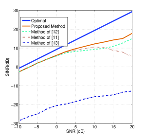
Figure 2: Example 1: Output SINR versus SNR.

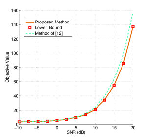
Figure 3: Example 1: Objective function of the problem (13) versus SNR.

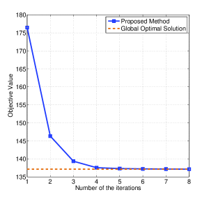
Figure 4: Example 1: Objective function of the problem (13) versus the number of iterations.

V-B Simulation Example 2

In this example, we also consider the locally incoherently scattered desired and interference sources. However, compared to the previous example, there is a substantial error in the knowledge of the desired source angular power density.

The interference source is modeled as in the previous example, while the angular power density of the desired source is assumed to be a truncated Laplacian function distorted by severe fluctuations. The central angle and the scale parameter of the Laplacian distribution is assumed to be $30^{\circ}$ and $0.1$, respectively, and it is assumed to be equal to zero outside of the interval $[15^{\circ},45^{\circ}]$ as it has been shown in Fig. 5. The presumed knowledge of the desired source is different from the actual one and is characterized by an incoherently scattered source with Gaussian angular power density whose central angle and angular spread are $32^{\circ}$ and $1^{\circ}$, respectively.

Figs. 6 and 7 depict the corresponding output SINR and the objective function values of the problem (13) obtained by the beamforming methods tested versus SNR. Form these figures, it can be concluded that the proposed new method has superior performance over the other methods as well as it achieves the global minimum of the optimization problem (13)

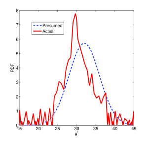
Figure 5: Example 2: Actual and presumed angular power densities of general-rank source.

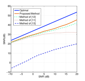
Figure 6: Example 2: Output SINR versus SNR.

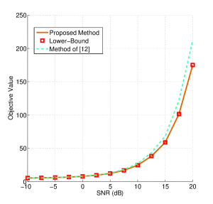
Figure 7: Example 2: Objective function of the problem (13) versus SNR.

V-C Simulation Example 3

In this example, we compare the efficiency of the proposed POTDC method to that of the DC iteration-based method that can be written for the problem under consideration as

$$\min\limits_{\mathbf{w}} \mathbf{w}^{H}(\mathbf{\hat{R}}+\gamma\mathbf{I})\mathbf{w}$$ (32)

$${\rm s.t.} \!\!f(\mathbf{w}^{(k)})\!+\!\langle\bigtriangledown f(\mathbf{w}^{(k)},\mathbf{w}-\mathbf{w}^{(k)})\rangle\!-\!\eta\|\mathbf{w}\|\!\geq\!1$$

where the function $f(\mathbf{w})=\|\mathbf{Q}\mathbf{w}\|$ is replaced with the first two terms of the Taylor expansion of $f(\mathbf{w})$ around $\mathbf{w}^{(k)}$. At the first iteration $\mathbf{w}^{(1)}$ is initialized and in the next iterations $\mathbf{w}^{(k)}$ is selected as the optimal $\mathbf{w}$ obtained from solving (32) in the previous iteration. Thus, the iteration are performed over the whole vector of variables of the problem.

The simulation set up is the same as in our Simulation example 1 except that different number of antennas are used. For a fair comparison, the initial point $\alpha_{0}$ in the proposed POTDC method and $\mathbf{w}^{(1)}$ in (32) are chosen randomly. Table I shows the average number of the iterations for the aforementioned methods versus the size of the antenna array. The accuracy is set to $10^{-6}$, $SNR=-10$ dB, and each number in the table is obtained by averaging the results from 200 runs. From this table, it can be seen that the number of the iterations for the POTDC method is almost fixed while it increases for the DC-iteration method as the size of the array increases. The latter phenomenon can be justified by considering the DC iteration-type interpretation of the POTDC method over the one dimensional function of $k(\alpha)$. The dimension of $k(\alpha)$ is independent of the size of the array (thus, the size of the optimization problem), while the size of search space for the DC iteration-based method (32), that is, $2M$, increases as the size of the array increases.

TABLE I: Average number of the iterations

Array size	8	10	12	14	16	18	20
POTDC	2.940	2.855	2.805	2.835	2.870	2.840	2.920
DC iteration	5.930	6.925	7.870	9.180	10.430	11.890	13.305

The average (over 200 runs) CPU time for the aforementioned methods is also compared in Table 2. Both methods have been implemented in Matlab using CVX software and run on the same desktop with Pentium(R) 4 CPU 3.40 GHz.

TABLE II: Average CPU time

Array size	8	10	12	14	16	18	20
POTDC	0.851	0.867	0.939	1.056	1.153	1.269	1.403
DC iteration	4.353	3.897	5.882	5.366	7.870	8.575	10.041

Table 2 confirms that the proposed method is more efficient that the DC iteration-based one in terms of the time which is spent for solving the same problem. Note that although the number of variables in the matrix $\mathbf{W}$ of the optimization problem (29) is in general $M^{2}+1$ (since $\mathbf{W}$ has to be a Hermitian matrix) after the rank one constraint is relaxed, the probability that the optimal $\mathbf{W}$ is rank one has been shown to be very high [10], [24]-[26]. It is also approved by this our simulations. Thus, in almost all cases, for different data sets, the actual dimension of the problem (29) is $2M+1$. As a result, the average complexity of solving (29) is significantly smaller than the worst-case complexity.

VI Conclusion

We have considered the RAB problem for general-rank signal model with additional positive semi-definite constraint. Such RAB problem corresponds to a non-convex DC optimization problem. We have studied this non-convex DC problem rigorously and designed the POTDC algorithm for solving it. It has been proved that the point found by the POTDC algorithm for RAB for general-rank signal model with positive semi-definite constraint is a KKT optimal point. Moreover, there is a strong evidence that the POTDC method actually finds the globally optimal point of the problem under consideration, which is shown in terms of a number of lemmas and one conjecture. Specifically, we have proved a number of results that lead us to the equivalence between the claim of global optimality for the POTDC algorithm as applied to the problem under consideration and the convexity of the one-dimensional optimal value function (26). The latter convexity has been checked numerically by using the convexity on lines property of convex functions. The fact that enables such numerical check is that the argument of this one-dimensional optimal value function is proved to take values only in a closed interval. The resulted RAB method shows superior performance compared to the other existing methods in terms of the output SINR. It also has lower average overall complexity than the other traditional methods that can be used for the same optimization problem such as, for example, the DC iteration-based method. None of the existing methods used for DC programming problems, however, guarantee that the problem can be solved in polynomial time. Thus, the fundamental development of this work is that the claim of global optimality of the proposed POTDC method boils down to one conjecture that can be easily checked numerically. It implies that certain relatively simple DC programming problems (an example of such problem is the RAB for general-rank signal model with additional positive semi-definite constraint), which are believed to be NP-hard, are likely not NP-hard.

VII Appendix

VII-A Proof of Lemma 1

Since the objective function as well as the constraints of the optimization problem (9) are all quadratic functions of $\mathbf{\Delta}$, this problem is convex. It is easy to verify that this problem satisfies the Slater’s constraint qualification and as a result the KKT conditions are necessary and sufficient optimality conditions. Let us introduce the Lagrangian as

$$L(\mathbf{\Delta},\mu)\!\!\!\! = \!\!\!\!\mathbf{w}^{H}\left(\mathbf{Q}^{H}\mathbf{Q}+\mathbf{Q}^{H}\mathbf{\Delta}+\mathbf{\Delta}^{H}\mathbf{Q}+\mathbf{\Delta}^{H}\mathbf{\Delta}\right)\mathbf{w}$$ (33)

$$+\ \mu(\|\mathbf{\Delta}\|^{2}-\eta^{2})$$

where $\mu$ is the non-negative Lagrange multiplier. The KKT optimality conditions are

$$\boldsymbol{\nabla}_{\mathbf{\Delta}}L(\mathbf{\Delta},\mu)=\mathbf{0}$$ (34a)

$$\|\mathbf{\Delta}\|^{2}\leq\eta^{2}$$ (34b)

$$\mu(\|\mathbf{\Delta}\|^{2}-\eta^{2})=0$$ (34c)

$$\mu\geq 0.$$ (34d)

where $\mathbf{0}$ is the vector of zeros. Using the matrix differentiation, the zero gradient condition (34a) can be expressed as $\mathbf{Q}\mathbf{w}\mathbf{w}^{H}+\boldsymbol{\Delta}\mathbf{w}\mathbf{w}^{H}+\mu\boldsymbol{\Delta}=\mathbf{0}$ or, equivalently, as

$$\mathbf{\Delta}=-\mathbf{Q}\mathbf{w}\mathbf{w}^{H}(\mathbf{w}\mathbf{w}^{H}+\mu\mathbf{I})^{-1}.$$ (35)

Moreover, using the matrix inversion lemma, the expression (35) can be simplified as

$$\mathbf{\Delta}=-\frac{\mathbf{Q}\mathbf{w}\mathbf{w}^{H}}{\|\mathbf{w}\|^{2}+\mu}.$$ (36)

The Lagrange multiplier $\mu$ can be determined based on the conditions (34b)–(34d). For this goal, we find a simpler expression for the norm of the matrix $\mathbf{Q}\mathbf{w}\mathbf{w}^{H}$ as follows

$$\|\mathbf{Q}\mathbf{w}\mathbf{w}^{H}\|^{2}\!\! = \!\!{\rm tr}\{\mathbf{Q}\mathbf{w}\mathbf{w}^{H}\mathbf{w}\mathbf{w}^{H}\mathbf{Q}^{H}\}$$ (37)

$$= \!\!{\rm tr}\{\mathbf{Q}\mathbf{w}\mathbf{w}^{H}\mathbf{Q}^{H}\}\cdot\mathbf{w}^{H}\mathbf{w}$$

$$= \!\!\|\mathbf{Q}\mathbf{w}\|^{2}\|\mathbf{w}\|^{2}$$

Using (37), it can be obtained that

$$\delta(\mu)\triangleq\|\mathbf{\Delta}\|=\frac{\|\mathbf{Q}\mathbf{w}\|\|\mathbf{w}\|}{\|\mathbf{w}\|^{2}+\mu}.$$ (38)

where the new function $\delta(\mu)$ is defined for notation simplicity. It is easy to verify that $\delta(\mu)$ is a strictly decreasing function with respect to $\mu\geq 0$. Consequently, for any arbitrary $\mu\geq 0$, it is true that $\delta(\mu)\leq\delta(0)=\|\mathbf{Q}\mathbf{w}\|/\|\mathbf{w}\|$. Depending on whether $\delta(0)$ is less than or equal to $\eta$ or not, the following two cases are possible. If $\delta(0)\leq\eta$, then $\mu$ and $\boldsymbol{\Delta}$ can be found as $\mu=0$ and $\boldsymbol{\Delta}=-\mathbf{Q}\mathbf{w}\mathbf{w}^{H}/\|w\|^{2}$, which is obtained by simply substituting $\mu=0$ in (36). In this case, the KKT conditions (34b)–(34d) are obviously satisfied. In the other case, when $\delta(0)>\eta$, the above obtained $\mathbf{\Delta}$ for $\mu=0$ does not satisfy the condition (34b) because $\|\mathbf{\Delta}\|=\delta(0)>\eta$. Since, $\delta(\mu)$ is a strictly decreasing function with respect to $\mu\geq 0$, for satisfying (34b), the value of $\mu$ must be strictly larger than zero and as a result the condition (34c) implies that $\|\mathbf{\Delta}\|=\eta$. Note that if $\mu>0$ and $\|\mathbf{\Delta}\|$ obtained by substituting such $\mu$ in (36) is equal to $\eta$, then the KKT conditions (34b)–(34d) are all satisfied. Thus, we need to find the value of $\mu$ such that the corresponding $\|\mathbf{\Delta}\|$ is equal to $\eta$. By equating $\delta(\mu)$ to $\eta$, it can be resulted that $\mu_{0}=\|\mathbf{w}\|/\eta\cdot(\|\mathbf{Q}\mathbf{w}\|-\eta\|\mathbf{w}\|)$. Considering the above two cases together, the optimal $\mathbf{\Delta}$ can be expressed as

$$\mathbf{\Delta}=\left\{\begin{array}[]{ll}-\eta\frac{\mathbf{Q}\mathbf{w}\mathbf{w}^{H}}{\|\mathbf{Q}\mathbf{w}\|\|\mathbf{w}\|},&\quad\|\mathbf{Q}\mathbf{w}\|\geq\eta\|\mathbf{w}\|\\ -\frac{\mathbf{Q}\mathbf{w}\mathbf{w}^{H}}{\|\mathbf{w}\|^{2}},&\quad\ \mbox{otherwise.}\end{array}\right.$$ (41)

Finally, substituting (41) in the objective function of the problem (9), the worst-case signal power for a fixed beamforming vector $\mathbf{w}$ can be found as shown in (12). $\hfill\blacksquare$

VII-B Proof of Lemma 2

Let $(\mathbf{w}_{\rm opt},\alpha_{\rm opt})$ denote the optimal solution of the problem (14). Let us define the following auxiliary optimization problem based on the problem

$$\min_{\mathbf{w}} \,\mathbf{w}^{H}(\hat{\mathbf{R}}+\gamma\mathbf{I})\mathbf{w}\quad$$

$${\rm s.t.} \mathbf{w}^{H}\mathbf{Q}^{H}\mathbf{Q}\mathbf{w}=\alpha_{\rm opt}$$ (42)

$$\mathbf{w}^{H}\mathbf{w}\leq\frac{(\sqrt{\alpha_{\rm opt}}-1)^{2}}{\eta^{2}}.$$

It can be seen that if $\mathbf{w}$ is a feasible point of the problem (42), then the pair $(\mathbf{w},\alpha_{\rm opt})$ is also a feasible point of the problem (14) which implies that the optimal value of the problem (42) is greater than or equal to that of (14). However, since $\mathbf{w}_{\rm opt}$ is a feasible point of the problem (42) and the value of the objective function at this feasible point is equal to the optimal value of the problem (14), i.e., it is equivalent to $\mathbf{w}_{\rm opt}^{H}(\hat{\mathbf{R}}+\gamma\mathbf{I})\mathbf{w}_{\rm opt}$, it can be concluded that both of the optimization problems (14) and (42) have the same optimal value. Let us define another auxiliary optimization problem based on the problem (42) as

$$g\triangleq \min\limits_{\mathbf{w}} \,\mathbf{w}^{H}(\hat{\mathbf{R}}+\gamma\mathbf{I})\mathbf{w}\quad$$ (43)

$${\rm s.t.} \mathbf{w}^{H}\mathbf{Q}^{H}\mathbf{Q}\mathbf{w}=\alpha_{opt}$$

which is obtained from (42) by dropping the last constraint of (42). The feasible set of the optimization problem (42) is a subset of the feasible set of the optimization problem (43). As a result, the optimal value $g$ of the problem (43) is smaller than or equal to the optimal value of the problem (42), and thus also, the optimal value of the problem (14). Using the maxmin theorem [23], it is easy to verify that $g=\alpha_{opt}/\lambda_{\rm max}\left\{(\hat{\mathbf{R}}+\gamma\mathbf{I})^{-1}\mathbf{Q}^{H}\mathbf{Q}\right\}$. Since $g$ is smaller than or equal to the optimal value of the problem (14), it is upper-bounded by $\mathbf{w}_{0}^{H}(\hat{\mathbf{R}}+\gamma\mathbf{I})\mathbf{w}_{0}$, where $\mathbf{w}_{0}$ is an arbitrary feasible point of (14). The latter implies that $\alpha_{opt}\leq\lambda_{\rm max}\left\{(\hat{\mathbf{R}}+\gamma\mathbf{I})^{-1}\mathbf{Q}^{H}\mathbf{Q}\right\}\cdot\mathbf{w}_{0}^{H}(\hat{\mathbf{R}}+\gamma\mathbf{I})\mathbf{w}_{0}$. $\hfill\blacksquare$

VII-C Proof of Lemma 3

It is easy to verify that the dual problem for both optimization problems of $h(\alpha)$ and $k(\alpha)$ is the same and it can be expressed for fixed $\alpha$ as

$$\max\limits_{\tau,\psi} \tau\alpha-\psi(\sqrt{\alpha}-1)^{2}/\eta^{2}$$

$${\rm s.t.} (\hat{\mathbf{R}}+\gamma\mathbf{I})-\tau\cdot\mathbf{Q}^{H}\mathbf{Q}+\psi\mathbf{I}\succeq\mathbf{0}$$ (44)

$$\psi\geq 0$$

where $\tau$ and $\psi$ are the Lagrange multipliers. Based on the dual problem (44), a new optimal value function is defined as

$$d(\alpha)\!\! \triangleq \!\!\Big{\{}\max\limits_{\tau,\psi}\tau\alpha-\psi\frac{(\sqrt{\alpha}-1)^{2}}{\eta^{2}}\ |\ (\hat{\mathbf{R}}+\gamma\mathbf{I})$$ (45)

$$- \!\!\tau\mathbf{Q}^{H}\mathbf{Q}+\psi\mathbf{I}\succeq\mathbf{0},\ \psi\geq 0\Big{\}}.$$

The optimization problem of $k(\alpha)$ is a convex SDP problem which satisfies the Slater’s conditions as $\tau=0$ and $\psi=1$ is a strictly feasible point for its dual problem (44). Thus, the duality gap between the optimization problem of $h(\alpha)$, i.e., the problem (23) and its dual problem (44) is zero. It implies that

$$k(\alpha)=d(\alpha),\quad\alpha\in[\theta_{1},\theta_{2}].$$ (46)

On the other hand, the optimization problem of $h(\alpha)$ is specifically a quadratically constrained quadratic programming (QCQP) problem with only two constraints. It has been recently shown that the duality gap between a QCQP in complex variables with two constraints and its dual problem is zero [27], [28]. Based on the latter fact, it can be obtained that

$$h(\alpha)=d(\alpha),\quad\alpha\in[\theta_{1},\theta_{2}].$$ (47)

Using (46) and (47), it can be concluded that the functions $h(\alpha)$ and $k(\alpha)$ are equivalent.

Let $\mathbf{w}_{\alpha}$ denote the optimal solution of the optimization problem of $h(\alpha)$ which implies that $h(\alpha)=\mathbf{w}_{\alpha}^{H}(\hat{\mathbf{R}}\!+\!\gamma\mathbf{I})\mathbf{w}_{\alpha}$. It is then trivial to verify that $\mathbf{W}_{\alpha}\triangleq\mathbf{w}_{\alpha}\mathbf{w}_{\alpha}^{H}$ is a feasible point of the optimization problem of $k(\alpha)$ and ${\rm tr}\left\{(\hat{\mathbf{R}}+\gamma\mathbf{I})\mathbf{W}_{\alpha}\right\}=h(\alpha)$. Using the fact that $h(\alpha)$ and $k(\alpha)$ are equivalent, it can be concluded that ${\rm tr}\left\{(\hat{\mathbf{R}}+\gamma\mathbf{I})\mathbf{W}_{\alpha}\right\}=k(\alpha)$ which implies that $\mathbf{W}_{\alpha}$ is the optimal solution of the optimization problem of $k(\alpha)$. The latter means that, for a fixed value of $\alpha$, the optimization problem of $k(\alpha)$ has always a rank-one solution. A method for extracting a rank-one solution from a general-rank solution of QCQP is explained, for example, in [28]. It is trivial to see that the scaled dominant eigenvector of such a rank-one solution of the optimization problem of $k(\alpha)$ is the optimal solution of the optimization problem of $h(\alpha)$. $\hfill\blacksquare$

VII-D Proof of Lemma 4

First, we prove that $l(\alpha,\alpha_{c})$ is a convex function with respect to $\alpha$. For this goal, let $\mathbf{W}_{\alpha_{1}}$ and $\mathbf{W}_{\alpha_{2}}$ denote the optimal solution of the optimization problems of $l(\alpha_{1},\alpha_{c})$ and $l(\alpha_{2},\alpha_{c})$, respectively, i.e., $l(\alpha_{1},\alpha_{c})={\rm tr}\left\{(\hat{\mathbf{R}}+\gamma\mathbf{I})\mathbf{W}_{\alpha_{1}}\right\}$ and $l(\alpha_{2},\alpha_{c})={\rm tr}\left\{(\hat{\mathbf{R}}+\gamma\mathbf{I})\mathbf{W}_{\alpha_{2}}\right\}$, where $\alpha_{1}$ and $\alpha_{2}$ are any two arbitrary points in the interval $[\theta_{1},\theta_{2}]$. It is trivial to verify that $\theta\mathbf{W}_{\alpha_{1}}+(1-\theta)\mathbf{W}_{\alpha_{2}}$ is a feasible point of the corresponding optimization problem of $l(\theta\alpha_{1}+(1-\theta)\alpha_{2},\alpha_{c})$ (see the definition (30)). Therefore,

$$l(\theta\alpha_{1}\!\!\!\! + \!\!\!\!\!(1\!-\!\theta)\alpha_{2},\alpha_{c})$$ (48)

$$\leq{\rm tr}\big{\{}(\hat{\mathbf{R}}\!+\!\gamma\mathbf{I})(\theta\mathbf{W}_{\alpha_{1}}\!\!+\!(1\!-\!\theta)\mathbf{W}_{\alpha_{2}})\big{\}}$$

$$=\theta{\rm tr}\big{\{}(\hat{\mathbf{R}}+\gamma\mathbf{I})\mathbf{W}_{\alpha_{1}}\big{\}}$$

$$\ \ +(1-\theta){\rm tr}\big{\{}(\hat{\mathbf{R}}+\gamma\mathbf{I})\mathbf{W}_{\alpha_{2}}\big{\}}$$

$$=\theta l(\alpha_{1},\alpha_{c})+(1-\theta)l(\alpha_{2},\alpha_{c})$$

which proves that $l(\alpha,\alpha_{c})$ is a convex function with respect to $\alpha$.

In order to show that $l(\alpha,\alpha_{c})$ is greater than or equal to $k(\alpha)$, it suffices to show that the feasible set of the optimization problem of $l(\alpha,\alpha_{c})$ is a subset of the feasible set of the optimization problem of $k(\alpha)$. Let $\mathbf{W}_{1}$ denote a feasible point of the optimization problem of $l(\alpha,\alpha_{c})$, it is easy to verify that $\mathbf{W}_{1}$ is also a feasible point of the optimization problem of $k(\alpha)$ if the inequality $\sqrt{\alpha}\leq\sqrt{\alpha_{c}}+\frac{\alpha-\alpha_{c}}{2\sqrt{\alpha_{c}}}$ holds. This inequality can be rearranged as

$$(\sqrt{\alpha}-\sqrt{\alpha_{c}})^{2}\geq 0$$ (49)

and it is valid for any arbitrary $\alpha$. Therefore, $\mathbf{W}_{1}$ is also a feasible point of the optimization problem of $k(\alpha)$ which implies that $l(\alpha,\alpha_{c})\geq k(\alpha)$.

In order to show that the right and left derivatives are equal, we use the result of [29, Theorem 10] which gives expressions for the directional derivatives of a parametric SDP. Specifically, in [29, Theorem 10] the directional derivatives for the following optimal value function

$$\psi(\mathbf{u})\triangleq\{\min\limits_{\mathbf{y}}f(\mathbf{y},\mathbf{u})\ |\ \mathbf{G}(\mathbf{y},\mathbf{u})\preceq\mathbf{0}_{n\times n}\}$$ (50)

are derived, where $f(\mathbf{y},\mathbf{u})$ and $\mathbf{G}(\mathbf{y},\mathbf{u})$ are a scaler and an $n\times n$ matrix, respectively, $\mathbf{y}\in{\cal R}^{m}$ is the optimization variables and $\mathbf{u}\in{\cal R}^{k}$ is the optimization parameters. Let $\mathbf{u}_{c}$ be an arbitrary fixed point. If the optimization problem of $\psi(\mathbf{u}_{c})$ poses certain properties, then according to [29, Theorem 10] it is directionally differentiable at $\mathbf{u}_{c}$. These properties are (i) the functions $f(\mathbf{y},\mathbf{u})$ and $\mathbf{G}(\mathbf{y},\mathbf{u})$ are continuously differentiable, (ii) the optimization problem of $\psi(\mathbf{u}_{c})$ is convex, (iii) the set of optimal solutions of the optimization problem of $\psi(\mathbf{u}_{c})$ denoted as $\cal M$ is nonempty and bounded, (iv) the Slater condition for the optimization problem of $\psi(\mathbf{u}_{c})$ holds true, and (v) the inf-compatness condition is satisfied. Here inf-compatness condition refers to the condition of the existence of $\alpha>\psi(\mathbf{u}_{c})$ and a compact set $S\subset{\cal R}^{m}$ such that $\{\mathbf{y}|f(\mathbf{y},\mathbf{u})\leq\alpha,\mathbf{G}(\mathbf{y},\mathbf{u})\preceq\mathbf{0}\}\subset S$ for all $\mathbf{u}$ in a neighborhood of $\mathbf{u}_{c}$. If for all $\mathbf{u}$ the optimization problem of $\psi(\mathbf{u})$ is convex and the set of optimal solutions of $\psi(\mathbf{u})$ is non-empty and bounded, then the inf-compactness conditions holds automatically.

The directional derivative of $\psi(\mathbf{u})$ at $\mathbf{u}_{c}$ in a direction $\mathbf{d}\in{\cal R}^{k}$ is given by

$$\psi^{\prime}(\mathbf{u}_{c},\mathbf{d})=\min\limits_{\mathbf{y}\in{\cal M}}\max\limits_{\boldsymbol{\Omega}\in{\cal Z}}\mathbf{d}^{T}\nabla_{\mathbf{u}}L(\mathbf{y},\boldsymbol{\Omega},\mathbf{u}_{c}),$$ (51)

where $\cal{Z}$ is the set of optimal solutions of the dual problem of the optimization problem of $\psi(\mathbf{u}_{c})$ and $L(\mathbf{y},\Omega,\mathbf{u})$ denotes the Lagrangian defined as

$$L(\mathbf{y},\Omega,\mathbf{u})\triangleq f(\mathbf{y},\mathbf{u})+{\rm tr}\left(\boldsymbol{\Omega}\cdot\mathbf{G}(\mathbf{y},\mathbf{u})\right)$$ (52)

where $\boldsymbol{\Omega}$ denotes the Lagrange multiplier matrix.

Let us look again to the definitions of the optimal value functions $k(\alpha)$ and $l(\alpha,\alpha_{c})$ (26) and (30), respectively, and define the following block diagonal matrix

$$\!\!\!\!\!\!\!\mathbf{G}_{1}(\mathbf{W},\alpha)=$$ (53)

$$\!\!\!\!\!\!\!\begin{pmatrix}-\mathbf{W}\!\!\!\!&\!\!\!\!\mathbf{0}\!\!\!\!\!\!\!\!\!\!\!&\!\!\!\!\!\!\!\!\!\!\!\!\!\mathbf{0}\!\!\!\!\!\!\!\!\!&\!\!\!\!\!\!\!\!\!\mathbf{0}\\ \mathbf{0}\!\!\!\!&\!\!\!\!{\eta^{2}}{\rm tr}\{\mathbf{W}\}\!-\!{(\sqrt{\alpha}\!-\!1)^{2}}\!\!\!\!\!\!\!\!\!\!\!&\!\!\!\!\!\!\!\!\!\!\!\!\!0\!\!\!\!\!\!\!\!\!&\!\!\!\!\!\!\!\!\!0\\ \mathbf{0}\!\!\!\!&\!\!\!\!\!\!\!0\!\!\!\!\!\!\!\!\!\!\!&\!\!\!\!\!\!\!\!\!\!\!\!\!{\rm tr}\{\mathbf{Q}^{H}\mathbf{Q}\mathbf{W}\}-\alpha\!\!\!\!\!\!\!\!\!&\!\!\!\!\!\!\!\!\!0\\ \mathbf{0}\!\!\!\!&\!\!\!\!\!\!\!0\!\!\!\!\!\!\!\!\!\!\!&\!\!\!\!\!\!\!\!\!\!\!\!\!0\!\!\!\!\!\!\!\!\!&\!\!\!\!\!\!\!\!\!\alpha-{\rm tr}\{\mathbf{Q}^{H}\mathbf{Q}\mathbf{W}\}\end{pmatrix}$$

as well as another block diagonal matrix denoted as $\mathbf{G}_{2}(\mathbf{W},\alpha)$ which has exactly same structure as the matrix $\mathbf{G}_{1}(\mathbf{W},\alpha)$ with only difference that the element ${\eta^{2}}{\rm tr}\{\mathbf{W}\}-{(\sqrt{\alpha}-1)^{2}}$ in $\mathbf{G}_{1}(\mathbf{W},\alpha)$ is replaced by ${\eta^{2}}\cdot{\rm tr}\{\mathbf{W}\!\}+{(\sqrt{\alpha_{c}}-1)+\alpha\left({1}/{\sqrt{\alpha_{c}}}-1\right)}$ in $\mathbf{G}_{2}(\mathbf{W},\alpha)$. Then the optimal value functions $k(\alpha)$ and $l(\alpha,\alpha_{c})$ can be equivalently recast as

$$k(\alpha)\!\!\! = \!\!\!\left\{\min\limits_{\mathbf{W}}{\rm tr}\left\{(\hat{\mathbf{R}}+\gamma\mathbf{I})\cdot\mathbf{W}\right\}\ |\mathbf{G}_{1}(\mathbf{W},\alpha)\preceq\mathbf{0}\right\},$$ (54)

$$\quad\theta_{1}\leq\alpha\leq\theta_{2}$$

and

$$l(\alpha,\alpha_{c})\!\!\! = \!\!\!\left\{\min\limits_{\mathbf{W}}{\rm tr}\left\{(\hat{\mathbf{R}}+\gamma\mathbf{I})\cdot\mathbf{W}\right\}\ |\mathbf{G}_{2}(\mathbf{W},\alpha)\preceq\mathbf{0}\right\},$$ (55)

$$\quad\theta_{1}\leq\alpha\leq\theta_{2}.$$

It is trivial to verify that the optimization problems of $k(\alpha_{c})$ and $l(\alpha_{c},\alpha_{c})$ can be expressed as

$$\min\limits_{\mathbf{W}} {\rm tr}\{(\hat{\mathbf{R}}+\gamma\mathbf{I})\cdot\mathbf{W}\}$$ (56)

$${\rm s.t.} \ {\rm tr}\{\mathbf{Q}^{H}\mathbf{Q}\mathbf{W}\}=\alpha_{c}$$

$$\ {\rm tr}\{\mathbf{W}\}\!\leq\!\frac{(\sqrt{\alpha_{c}}\!-\!1)^{2}}{\eta^{2}}$$

$$\ \mathbf{W}\succeq\mathbf{0}.$$

The problem (56) is convex and its solution set is non-empty and bounded. Indeed, let $\mathbf{W}_{1}$ and $\mathbf{W}_{2}$ denote two optimal solutions of the problem above. The Euclidean distance between $\mathbf{W}_{1}$ and $\mathbf{W}_{2}$ can be expressed as

$$d(\mathbf{W}_{1},\mathbf{W}_{2})\!\!\! = \!\!\!\|\mathbf{W}_{1}-\mathbf{W}_{2}\|$$ (57)

$$= \!\!\!\sqrt{{\rm tr}\{\mathbf{W}_{1}^{2}\}+{\rm tr}\{\mathbf{W}_{2}^{2}\}-2{\rm tr}\{\mathbf{W}_{1}\mathbf{W}_{2}\}}$$

$$\leq \!\!\!\sqrt{2\frac{(\sqrt{\alpha_{c}}\!-\!1)^{4}}{\eta^{4}}}$$

where the last line is due to the fact that the matrix product $\mathbf{W}_{1}\mathbf{W}_{2}$ is positive semi-definite and, therefore, ${\rm tr}\{\mathbf{W}_{1}\mathbf{W}_{2}\}\geq 0$, and also the fact that for any arbitrary positive semi-definite matrix ${\rm tr}\{\mathbf{A}^{2}\}\leq{\rm tr}\{\mathbf{A}\}^{2}$. From the equation above, it can seen that the distance between any two arbitrary optimal solutions of (56) is finite and, therefore, the solution set is bounded. As it was mentioned in the proof of Lemma 2, the optimization problem (56) satisfies the strong duality. In a similar way, it can be shown that the inf-compactness condition is satisfied by verifying that the optimization problems of $k(\alpha)$ and $l(\alpha,\alpha_{c})$ are convex and their corresponding solution sets are bounded for any $\alpha$. Therefore, both of the optimal value functions $k(\alpha)$ and $l(\alpha,\alpha_{c})$ are directionally differentiable at $\alpha_{c}$.

Using the result of [29, Theorem 10], the directional derivatives of $k(\alpha)$ and $l(\alpha,\alpha_{c})$ can be respectively computed as

$$k^{\prime}(\alpha,d)=\min\limits_{\mathbf{W}\in{\cal M}}\max\limits_{\boldsymbol{\Omega}\in{\cal Z}}d\left({\rm tr}\big{\{}\boldsymbol{\Omega}\cdot\frac{d}{d\alpha}\mathbf{G}_{1}(\mathbf{W},\alpha)\big{|}_{\alpha=\alpha_{c}}\big{\}}\right)$$ (58)

and

$$l^{\prime}(\alpha,\alpha_{c},d)=\min\limits_{\mathbf{W}\in{\cal M}}\max\limits_{\boldsymbol{\Omega}\in{\cal Z}}d\left({\rm tr}\big{\{}\boldsymbol{\Omega}\cdot\frac{d}{d\alpha}\mathbf{G}_{2}(\mathbf{W},\alpha)\big{|}_{\alpha=\alpha_{c}}\big{\}}\right)$$ (59)

where ${\cal M}$ and ${\cal Z}$ denote the optimal solution sets of the optimization problem of (56) and its dual problem, respectively. Using the definitions of $\mathbf{G}_{1}(\mathbf{W},\alpha)$ and $\mathbf{G}_{2}(\mathbf{W},\alpha)$, it can be seen that the terms ${d}\mathbf{G}_{1}(\mathbf{W},\alpha)/{d\alpha}$ and ${d}\mathbf{G}_{1}(\mathbf{W},\alpha)/{d\alpha}$ are equal at $\alpha=\alpha_{c}$ and, therefore, the directional derivatives are equivalent. The latter implies that the left and right derivatives of $k(\alpha)$ and $l(\alpha,\alpha_{c})$ are equal at $\alpha=\alpha_{c}$. $\hfill\blacksquare$

VII-E Proof of Lemma 5

i) As it has been explained, the optimization problem in Algorithm 1 at iteration $i,\ i\geq 2$ is obtained by linearizing $\sqrt{\alpha}$ at $\alpha_{opt,i-1}$. Since $\mathbf{W}_{opt,i-1}$ and $\alpha_{opt,i-1}$ are feasible for the optimization problem at iteration $i$, it can be straightforwardly concluded that the optimal value of the objective at iteration $i$ is less than or equal to the optimal value at the previous iteration, i.e., ${\rm tr}\left\{(\hat{\mathbf{R}}+\gamma\mathbf{I})\mathbf{W}_{opt,i}\right\}\leq{\rm tr}\left\{(\hat{\mathbf{R}}+\gamma\mathbf{I})\mathbf{W}_{opt,i-1}\right\}$ which completes the proof.

ii) Since the sequence of the optimal values, i.e., ${\rm tr}\left\{(\hat{\mathbf{R}}+\gamma\mathbf{I})\mathbf{W}_{opt,i}\right\},i\geq 1$ is non-increasing and bounded from below (every optimal value is non-negative), the sequence of the optimal values converges.

iii) The proof follows straightforwardly from Proposition 3.2 of [30, Section 3]. $\hfill\blacksquare$

References

- [1] A. B. Gershman, “Robust adaptive beamforming in sensor arrays,” Int. Journal of Electronics and Communications, vol. 53, no. 6, pp. 305-314, Dec. 1999.
- [2] S. A. Vorobyov, A. B. Gershman, and Z-Q. Luo, “Robust adaptive beamforming using worst-case performance optimization: A solution to the signal mismatch problem,” IEEE Trans. Signal Process., vol. 51, pp. 313-324, Feb. 2003.
- [3] J. Li, P. Stoica, and Z. Wang, “On robust Capon beamforming and diagonal loading,” IEEE Trans. Signal Process., vol. 51, pp. 1702 -1715, July 2003.
- [4] S. A. Vorobyov, A. B. Gershman, Z-Q. Luo, and N. Ma, “Adaptive beamforming with joint robustness against mismatched signal steering vector and interference nonstationarity,” IEEE Signal Process. Letters, vol. 11, no. 2, pp. 108-111, Feb. 2004.
- [5] J. Li, P. Stoica, and Z. Wang, “Doubly constrained robust Capon beamformer,” IEEE Trans. Signal Process., vol. 52, pp. 2407- 2423, Sep. 2004.
- [6] R. G. Lorenz and S. P. Boyd, “Robust minimum variance beamforming,” IEEE Trans. Signal Process., vol. 53, pp. 1684- 1696, May 2005.
- [7] S. A. Vorobyov, H. Chen, and A. B. Gershman, “On the relationship between robust minimum variance beamformers with probabilistic and worst-case distrortionless response constraints,” IEEE Trans. Signal Process., vol. 56, pp. 5719-5724, Nov. 2008.
- [8] A. Hassanien, S. A. Vorobyov, and K. M. Wong, “Robust adaptive beamforming using sequential programming: An iterative solution to the mismatch problem,” IEEE Signal Process. Letters, vol. 15, pp. 733-736, 2008.
- [9] A. Khabbazibasmenj, S. A. Vorobyov, and A. Hassanien, “Robust adaptive beamforming via estimating steering vector based on semidefinite relaxation,” in Proc. 44th Annual Asilomar Conf. Signals, Systems, and Computers, Pacific Grove, California, USA, Nov. 2010, pp. 1102-1106.
- [10] A. Khabbazibasmenj, S. A. Vorobyov, and A. Hassanien, “Robust adaptive beamforming based on steering vector estimation with as little as possible prior information,” IEEE Trans. Signal Process., vol. 60, pp. 2974–2987, June 2012.
- [11] S. Shahbazpanahi, A. B. Gershman, Z-Q. Luo, and K. M. Wong, “Robust adaptive beamforming for generalrank signal models,” IEEE Trans. Signal Process., vol. 51, pp. 2257-2269, Sept. 2003.
- [12] H. H. Chen and A. B. Gershman, “Robust adaptive beamforming for general-rank signal models with positive semi-definite constraints,” in Proc. IEEE ICASSP, Las Vegas, USA, Apr. 2008, pp. 2341-2344.
- [13] C. W. Xing, S. D. Ma, and Y. C. Wu, “On low complexity robust beamforming with positive semidefinite constraints,” IEEE Trans. Signal Process., vol. 57, pp. 4942 -4945, Dec. 2009.
- [14] H. H. Chen and A. B. Gershman, “Worst-case based robust adaptive beamforming for general-rank signal models using positive semi-definite covariance constraint,” in Proc. IEEE ICASSP, Prauge, Czech Republic, May. 2011, pp. 2628-2631.
- [15] A. Khabbazibasmenj and S. A. Vorobyov, “A computationally efficient robust adaptive beamforming for general-rank signal models with positive semi-definitness constraint,” in Proc. IEEE CAMSAP, San Juan, Puerto Rico, Dec. 2011, pp. 185-188.
- [16] A. Khabbazibasmenj, S. A. Vorobyov, F. Roemer, and M. Haardt, “Polynomial-time DC (POTDC) for sum-rate maximization in two-way AF MIMO relaying,” in Proc. IEEE ICASSP, Kyoto, Japan, Mar. 2012, pp. 2889-2892.
- [17] A. Khabbazibasmenj, F. Roemer, S. A. Vorobyov, and M. Haardt, “Sum-rate maximization in two-way AF MIMO relaying: Polynomial time solutions to a class of DC programming problems,” IEEE Trans. Signal Process., to appear Oct. 2012.
- [18] A. Pezeshki, B. D. Van Veen, L. L. Scharf, H. Cox, and M. Lundberg, “Eigenvalue beamforming using a multi-rank MVDR beamformer and subspace selection,” IEEE Trans. Signal Process., vol. 56, pp. 1954- 1967, May 2008.
- [19] R. Horst, P. M. Pardalos, and N. V. Thoai, Introduction to Global Optimization. Dordrecht, Netherlands: Kluwer Academic Publishers, 1995.
- [20] R. Horst and H. Tuy, Global Optimization: Deterministic Approaches. Springer, 1996.
- [21] J. Zhang, F. Roemer, M. Haardt, A. Khabbazibasmenj, and S. A. Vorobyov, “Sum rate maximization for multi-pair two-way relaying with single-antenna amplify and forward relays,” in Proc. 37th IEEE Inter. Conf. Acoustics, Speech, and Signal Processing, Kyoto, Japan, Mar. 2012, pp. 2477-2480.
- [22] A. L. Yuille and A. Rangarajan, “The concave-convex procedure,” Neural Computation, vol. 15, pp. 915-936, 2003.
- [23] S. Haykin, Adaptive Filter Theory. (3rd Edition). Prentice Hall, 1995.
- [24] Z.-Q. Luo, W.-K. Ma, A. M.-C. So, Y. Ye, and S. Zhang, “Semidefinite relaxation of quadratic optimization problems,” IEEE Signal Process. Mag., vol. 27, no. 3, pp. 20–34, May 2010.
- [25] K. T. Phan, S. A. Vorobyov, N. D. Sidiropoulos, and C. Tellambura, “Spectrum sharing in wireless networks via QoS-aware secondary multicast beamforming,” IEEE Trans. Signal Process., vol. 57, pp. 2323–2335, Jun. 2009.
- [26] Z.-Q. Luo, N. D. Sidiropoulos, P. Tseng, and S. Zhang, “Approximation bounds for quadratic optimization with homogeneous quadratic constraints,” SIAM J. Optim., vol. 18, no. 1, pp. 1–28, Feb. 2007.
- [27] A. Beck and Y. C. Eldar, “Strong duality in nonconvex quadratic optimization with two quadratic constraints,” SIAM J. Optim., vol. 17, no. 3, pp. 844 860, 2006.
- [28] Y. Huang and D. P. Palomar, “Rank-constrained separable semidefinite programming with applications to optimal beamforming,” IEEE Trans. Signal Process., vol. 58, pp. 664-678, Feb. 2010.
- [29] A. Shapiro, “First and second order analysis of nonlinear semidefinite programs,” Math. Programming Ser. B, vol. 77, pp. 301–320, 1997.
- [30] A. Beck, A. Ben-Tal and L. Tetruashvili, “A sequential parametric convex approximation method with applications to nonconvex truss topology design problems,” Journal of Global Optimization, vol. 47, no. 1, pp. 29–51, 2010.