Dynamics and length distribution of microtubules under force and confinement

Abstract

We investigate the microtubule polymerization dynamics with catastrophe and rescue events for three different confinement scenarios, which mimic typical cellular environments: (i) The microtubule is confined by rigid and fixed walls, (ii) it grows under constant force, and (iii) it grows against an elastic obstacle with a linearly increasing force. We use realistic catastrophe models and analyze the microtubule dynamics, the resulting microtubule length distributions, and force generation by stochastic and mean field calculations; in addition, we perform stochastic simulations. Freely growing microtubules exhibit a phase of bounded growth with finite microtubule length and a phase of unbounded growth. The main results for the three confinement scenarios are as follows: (i) In confinement by fixed rigid walls, we find exponentially decreasing or increasing stationary microtubule length distributions instead of bounded or unbounded phases, respectively. We introduce a realistic model for wall-induced catastrophes and investigate the behavior of the average length as a function of microtubule growth parameters. (ii) Under a constant force the boundary between bounded and unbounded growth is shifted to higher tubulin concentrations and rescue rates. The critical force $f_{c}$ for the transition from unbounded to bounded growth increases logarithmically with tubulin concentration and the rescue rate, and it is smaller than the stall force. (iii) For microtubule growth against an elastic obstacle, the microtubule length and polymerization force can be regulated by microtubule growth parameters. For zero rescue rate, we find that the average polymerization force depends logarithmically on the tubulin concentration and is always smaller than the stall force in the absence of catastrophes and rescues. For a non-zero rescue rate, we find a sharply peaked steady-state length distribution, which is tightly controlled by microtubule growth parameters. The corresponding average microtubule length self-organizes such that the average polymerization force equals the critical force $f_{c}$ for the transition from unbounded to bounded growth. We also investigate the force dynamics if growth parameters are perturbed in dilution experiments. Finally, we show the robustness of our results against changes of catastrophe models and load distribution factors.

I Introduction

Microtubules (MTs) are one of the main components of the cytoskeleton in eukaryotic cells. Their static and dynamic properties are essential for many cellular processes. MTs serve as pathways for molecular motor proteins Vale1987 and contribute to cell stiffness How2001 . Dynamic MTs play a crucial role in the constant reorganization of the cytoskeleton, and single MTs can generate polymerization forces up to several pN DY97 . These forces are used in various intracellular positioning processes D05 , such as positioning of the cell nucleus daga2006 or chromosomes during mitosis , establishing cell polarity SD07 , or regulation of cell shapes Picone2010 ; Dehmelt2003 . In many cellular processes, MTs establish and maintain a characteristic length in response to forces exerted, for example, from the confining cell cortex Picone2010 .

The fast spatial reorganization of MTs is based on the dynamic instability: Polymerization phases are stochastically interrupted by catastrophes which initiate phases of fast depolymerization; fast depolymerization terminates stochastically in a rescue event followed again by a polymerization phase Mitch1984 . This complex dynamic behavior with catastrophes and rescue events is central to a rapid remodelling of MTs in the cytoskeleton, but it also affects their ability to generate polymerization forces. We will show that, in general, the dynamic instability decreases the average polymerization force of a single MT.

In this article we theoretically investigate the polymerization dynamics of a single MT under force or confinement and in the presence of the MT dynamic instability. We use a coarse-grained polymerization model with dynamic instability and characterize spatial and temporal behavior in three different scenarios, which mimic typical cellular environments that can also be reproduced in vitro: (i) Confinement: The MT is confined between fixed rigid walls, which cannot be deformed by the microtubule. Such confinement is realized in fixed solid chambers Faiv2008 . (ii) Constant force: A constant force is acting on the MT. Constant forces can be realized by optical tweezers with a force clamp control Schek2007 . (iii) Elastic obstacle: The microtubule grows against an elastic obstacle, which resists further growth by a force growing linearly with displacement. Elastic forces can be realized by optical tweezers without force clamp Kers2006 ; Laan2008 . For all three confinement scenarios (i)–(iii) we focus on the resulting length distributions of MTs and for scenarios (ii) and (iii), we calculate the polymerization force that a single MT can generate.

Dynamic MTs also initiate regulation processes or are subject to regulation. Dynamic MTs can activate or deactivate proteins upon contacting the cell membrane storer1999 , or they can activate actin polymerization within the cell cortex Mitch1988 ; Rod2003 . At the same time, polymerizing MTs are also targets of cellular regulation mechanisms Athale2008 , which affect their dynamic properties.

The dynamic instability of MTs enables various regulation mechanisms of MT dynamics. Catastrophes and rescues result from the hydrolysis of GTP-tubulin within MTs. When GTP-tubulin is incorporated into the tip of a growing MT, it forms a stabilizing GTP-cap. The loss of this GTP-cap due to hydrolysis of GTP-tubulin to GDP-tubulin, causes a catastrophe Mitch1984 . In living cells, there are various microtubule associated proteins (MAPs) that either stabilize or destabilize microtubules and regulate microtubule dynamics both spatially and temporally Nogales2000 . Recently, the importance of MAPs in connection with the plus end of growing MTs has been recognized Akhm2008 . Stabilizing MAPs bind to assembled MTs, thereby reducing the catastrophe rate or increasing the rescue rate. Destabilizing MAPs such as OP18/stathmin bind to GTP-tubulin dimers, thus decreasing the available GTP-tubulin concentration, which in turn decreases the growth velocity of the GTP-cap and makes catastrophes more likely. Therefore, such mechanisms can regulate basic parameters in our model, such as the available GTP-tubulin concentration or the rescue rate, and we will systematically study their influence on the generated polymerization force for the three confinement scenarios (i)–(iii).

The paper is structured as follows: In Sec. II, the MT model and the basic notation are introduced. We also discuss the catastrophe model and the underlying hydrolysis mechanism in the absence and in the presence of a resisting force. Section III deals with the simulation model. In Secs. IV, V, and VI, results for the three scenarios (i)–(iii) are presented and discussed. In Sec. VII, the elastic obstacle is reconsidered using an alternative catastrophe model based on experimental measurements to show that our results are robust with respect to this change in the catastrophe model. In Sec. VIII, we show that our results are also robust with respect to possible generalization of the force-velocity relation by introducing load-distribution factors. Section IX contains a final discussion and outlook.

II Microtubule model

II.1 Single MT dynamics

The MT dynamics in the presence of its dynamic instability is described in terms of probability densities and switching rates Verd1992 ; Dogt1993PRL . In the growing state, a MT polymerizes with average velocity $v_{+}$. The MT stochastically switches from a state of growth ($+$) to a state of shrinkage ($-$) with the catastrophe rate $\omega_{c}$. In the shrinking state, it rapidly depolymerizes with an average velocity $v_{-}\simeq 3\cdot 10^{-7}\,{\rm m/s}$ (Table 1). With the rescue rate $\omega_{r}$ the MT stochastically switches from a state of shrinkage back to a state of growth. We model catastrophes and rescues as Poisson processes such that $\langle\tau_{+}\rangle=1/\omega_{c}$ and $\langle\tau_{-}\rangle=1/\omega_{r}$ are the average times spent in the growing and shrinking states, respectively. The stochastic time evolution of an ensemble of independent MTs, growing along the x-axis, can be described by two coupled master equations for the probabilities $p_{+}(x,t)$ and $p_{-}(x,t)$ of finding a MT with length $x$ at time $t$ in a growing or shrinking state,

$$\partial_{t}p_{+}(x,t) =-\omega_{c}p_{+}(x,t)+\omega_{r}p_{-}(x,t)-v_{+}\partial_{x}p_{+}(x,t)$$ (1)

$$\partial_{t}p_{-}(x,t) =\omega_{c}p_{+}(x,t)-\omega_{r}p_{-}(x,t)+v_{-}\partial_{x}p_{-}(x,t).$$ (2)

In the following, we will always use a reflecting boundary at $x=0$: A MT shrinking back to zero length undergoes a forced rescue instantaneously. This corresponds to

$$v_{+}p_{+}(0,t)=v_{-}p_{-}(0,t).$$ (3)

A more refined model including a nucleating state has been considered in Ref. Mulder2012 . For a constant and fixed catastrophe rate $\omega_{c}$, eqs. (1) and (2) together with the boundary condition (3) can be solved analytically on the half-space $x>0$, and we can determine the overall probability density function (OPDF) of finding a MT with length $x$ at time $t$, $P(x,t)\equiv p_{+}(x,t)+p_{-}(x,t)$ Verd1992 ; Dogt1993PRL . The solution exhibits two different growth phases: a phase of bounded growth and a phase of unbounded growth.

In the phase of bounded growth the average length loss during a period of shrinkage, $v_{-}\langle\tau_{-}\rangle=v_{-}/\omega_{r}$, exceeds the average length gain during a period of growth, $v_{+}\langle\tau_{+}\rangle=v_{+}/\omega_{c}$. The steady-state solution of $P(x,t)$ assumes a simple exponential form $P(x)=|\lambda|^{-1}e^{-x/|\lambda|}$ with an average length $\langle x\rangle=|\lambda|$ and a characteristic length parameter

$$\lambda\equiv\frac{v_{+}v_{-}}{v_{+}\omega_{r}-v_{-}\omega_{c}},$$ (4)

with $\lambda^{-1}<0$ for bounded growth Verd1992 . The transition to the regime of unbounded growth takes place at $\lambda^{-1}=0$, where the average length gain during growth equals exactly the average length loss during shrinkage,

$$v_{+}\omega_{r}=v_{-}\omega_{c},$$ (5)

such that $\langle x\rangle$ diverges.

In the regime of unbounded growth ($\lambda>0$), the average length gain during a period of growth is larger than the average length loss during a period of shrinkage. There is no steady state solution, and for long times $P(x,t)$ asymptotically approaches a Gaussian distribution Verd1992

$$P(x,t)\approx\frac{1}{2\sqrt{\pi D_{J}t}}\exp\left(-\frac{(x-Jt)^{2}}{4D_{J}t}\right)$$ (6)

centered on an average length which approaches linear growth $\langle x\rangle\approx Jt$ with a mean velocity $J$ and with diffusively growing width $\langle x^{2}\rangle-\langle x\rangle^{2}\approx 2D_{J}t$ with a diffusion constant $D_{J}$. The average growth velocity is given by

$$J=\frac{v_{+}\omega_{r}-v_{-}\omega_{c}}{\omega_{r}+\omega_{c}}$$ (7)

because the asymptotic probabilities to be in a growing or shrinking state are $\pi_{+}=\omega_{r}/(\omega_{c}+\omega_{r})$ and $\pi_{-}=\omega_{c}/(\omega_{c}+\omega_{r})$, respectively. The diffusion constant $D_{J}$ is

$$D_{J}=\frac{\omega_{c}\omega_{r}(v_{+}+v_{-})^{2}}{(\omega_{c}+\omega_{r})^{3}}.$$ (8)

The transition between the two growth phases can be achieved by changing one of the four parameters of MT growth, $\omega_{c}$, $\omega_{r}$, $v_{+}$, or $v_{-}$. In the following, we will use catastrophe models, where the catastrophe rate $\omega_{c}$ is a function of the growth velocity $v_{+}$, which in turn is determined by the GTP-tubulin concentration via the GTP-tubulin on-rate $\omega_{\text{on}}$ (assuming a fixed off-rate $\omega_{\text{off}}$). Moreover, experimental data suggest that $v_{-}$ is fixed to values close to $\sim 10^{-7}$ m/s (Table 1). As a consequence, there are two tunable control parameters left, the GTP-tubulin concentration or, equivalently, the tubulin on-rate $\omega_{\text{on}}$ and the rescue rate $\omega_{r}$. These are the control parameters we will explore for MTs in confinements and under force. These parameters are also targets for regulation by MAPs, such as OP18/stathmin, which reduces $\omega_{\text{on}}$ by binding to GTP-tubulin dimers or MAP4, which increases the rescue rate $\omega_{r}$.

II.2 Force-dependent catastrophe rate

In a growing state, GTP-tubulin dimers are attached to any of the 13 protofilaments with the rate $\omega_{\text{on}}$, which is directly related to the GTP concentration. We explore a regime $\omega_{\text{on}}=30,...,100\,{\rm s^{-1}}$, see Table 1. GTP-tubulin dimers are detached with the rate $\omega_{\text{off}}=6\,{\rm s}^{-1}$ Janson2004 such that we can typically assume $\omega_{\text{on}}\gg\omega_{\text{off}}$. In the absence of force or restricting boundaries, the velocity of growth is given by

$$v_{+}(0)=d\left(\omega_{\text{on}}-\omega_{\text{off}}\right).$$ (9)

Here $d$ denotes the effective dimer size $d\approx 8\text{nm}/13\approx 0.6\,{\rm nm}$.

The classical view of the MT catastrophe mechanism is based on a purely chemical model of catastrophes, where the catastrophe rate $\omega_{c}$ is determined by the hydrolysis dynamics of GTP-tubulin Mitch1984 . When GTP-tubulin is incorporated into the tip of a growing MT, it forms a stabilizing GTP-cap. In a chemical model, the loss of this GTP-cap due to hydrolysis of GTP-tubulin to GDP-tubulin directly causes a catastrophe. However, recent research indicates that the “structural plasticity” of the MT lattice can play a role for the kinetics of catastrophes Kueh2009 . This structural plasticity mechanism is based on the assumption that GDP-tubulin prefers a curved configuration, which generates additional mechanical stresses in the MT by hydrolysis. Also in the presence of structural plasticity, the loss of the GTP-cap has a destabilizing effect, but the kinetics leading to a catastrophe can be more complicated because the initiation of a catastrophe event is similar to the nucleation of a crack in the stressed MT lattice within this model. In this article, we focus on purely chemical catastrophe models and neglect mechanical effects on the catastrophe kinetics.

Within a chemical catastrophe model, the loss of the GTP-cap due to hydrolysis of GTP-tubulin to GDP-tubulin triggers a catastrophe immediately. Therefore, the catastrophe rate $\omega_{c}$ is given by the first-passage rate to a state with vanishing GTP-cap and has been discussed within a model with cooperative hydrolysis Flyv1994PRL ; Flyv1996PRE , where GTP-tubulin is hydrolyzed by a combination of random and vectorial mechanisms; similar models have also been discussed for hydrolysis in F-actin Kier2009 ; Kier2010 . In random hydrolysis, GTP-tubulin is hydrolyzed at a random site within the GTP-cap with a rate per length $r\backsimeq 3.7\cdot 10^{6}\,{\rm m^{-1}s^{-1}}$, while in vectorial hydrolysis, only GTP-tubulin with adjacent GDP-tubulin is hydrolyzed. This results in hydrolysis fronts propagating through the microtubule with average velocity $v_{h}\backsimeq 4.2\cdot 10^{-9}\,{\rm m/s}$. The inverse catastrophe rate can then be calculated as the mean first-passage time to a state with zero cap length, as a function of hydrolysis parameters and $v_{+}$. With $v=v_{+}-v_{h}$, $D=0.5d(v_{+}+v_{h})$ and $\gamma=0.5vD^{1/3}r^{-1/3}$ the exact analytical result for the dimensionless catastrophe rate $\alpha=\omega_{c}D^{-1/3}r^{-2/3}$ is given by the smallest solution of

$$Ai^{\prime}(\gamma^{2}-\alpha)=-\gamma Ai(\gamma^{2}-\alpha).$$ (10)

Here $Ai$ denotes the first Airy function and $Ai^{\prime}$ its derivative Abramowitz . We solved eq. (10) numerically and obtained a high order polynomial for the function $\alpha=\alpha(\gamma)$. This polynomial is used in simulations and analytical calculations to compute the catastrophe rate $\omega_{c}=\alpha(\gamma)D^{1/3}r^{2/3}$ as a function of the growth velocity $v_{+}$, while the hydrolysis parameters $v_{h}$ and $r$ are fixed.

Under a force $F$, the tubulin on-rate $\omega_{\text{on}}$ is modified by an additional Boltzmann factor Pes1993 and the force-dependent growth velocity becomes

$$v_{+}(F)=d\left[\omega_{\text{on}}\exp{(-Fd/k_{B}T})-\omega_{\text{off}}\right].$$ (11)

Here $Fd$ is the work that has to be done against the force $F$ to incorporate a single dimer of size $d$; $k_{B}$ is the Boltzmann constant and $T=300$ K the temperature. In the following we use the dimensionless force

$$f\equiv F/F_{0}~{}~{}\mbox{with}~{}~{}F_{0}=k_{B}T/d,$$ (12)

in terms of which the force-dependent growth velocity is given by

$$v_{+}(f)=d\left[\omega_{\text{on}}e^{-f}-\omega_{\text{off}}\right].$$ (13)

The characteristic force $F_{0}$ has a value $F_{0}=k_{B}T/d\approx 7\,{\rm pN}$. The dimensionless stall force

$$f_{\text{stall}}=\ln\left(\omega_{\text{on}}/\omega_{\text{off}}\right)$$ (14)

is defined by the condition of vanishing growth velocity $v_{+}(f_{\text{stall}})=0$. We typically have $f_{\text{stall}}\simeq 1.5,...,3$ or $F_{\text{stall}}\simeq 10,...,20\,{\rm pN}$ for $\omega_{\text{on}}=30,...,100\,{\rm s^{-1}}$. The stall force is the maximal force that the MT can generate in the absence of catastrophes. We will investigate how the forces that can be generated in the presence of catastrophes compare to this stall force.

The velocity-dependence of the catastrophe rate as calculated from eq. (10) gives rise to a force-dependence $\omega_{c}=\omega_{c}(v_{+}(f))$. We assume that this is the only effect of force on the catastrophe rate Janson2003 . As a result, the catastrophe rate increases exponentially, when $v_{+}(f)$ is decreased by applying a force $f$, but a finite value is maintained at $v_{+}(f)=0$, which is $\omega_{c}(v_{+}=0)\approx 2.9\,{\rm s}^{-1}$. We assume that $v_{-}$ is independent of force. For qualitative approximations, the force-dependence of the catastrophe rate can be described by an exponential increase above the characteristic force $F_{0}$,

$$\omega_{c}(f)\sim\omega_{c}(f\!=\!0)e^{f},$$ (15)

In Sec.  VII we introduce an alternative catastrophe model which is based on experimental measurements. The exponential approximation (15) applies to the catastrophe model described above as well as to the alternative catastrophe model, see Fig. 11. Our results are robust for all catastrophe models with an exponential increase above the characteristic force $F_{0}$. Our results do not directly apply to more elaborate multi-step catastrophe models with more than two MT states Gardner2011 .

III Simulation Model

In the simulations we solve the stochastic Langevin-like equations of motion for the length $x(t)$ of a single MT using numerical integration with fixed time steps $\Delta t$ and including stochastic switching between growth and shrinkage. In a growing state $x(t)$ is increased by $v_{+}\Delta t$, while in a state of shrinkage, it is decreased by $v_{-}\Delta t$. In the growing state, $v_{+}$ is calculated from eq. (9) for zero force and from eq. (11) under force. In each time step a uniformly distributed random number $\xi\in[0,1]$ is compared to $\omega_{r,c}\Delta t$. If $\xi<\omega_{r,c}\Delta t$ the MT changes its state of growth. The catastrophe rate $\omega_{c}$ is calculated from the high order polynomial obtained from eq. (10) as mentioned above. To assure $\omega_{r,c}\Delta t\leq 1$ we used a time step $\Delta t=0.1\,{\rm s}$. During the simulations all parameters of growth, $d=0.6\,{\rm nm}$, $r=3.6\cdot 10^{6}\,{\rm m^{-1}s^{-1}}$, $v_{h}=4.2\cdot 10^{-9}\,{\rm m/s}$, $k_{B}=1.38\cdot 10^{-23}\,{\rm J/K}$, $T=300\,{\rm K}$, and $\omega_{\text{off}}=6\,{\rm s}^{-1}$, are fixed, see Table 2, except for $\omega_{\text{on}}$, which is varied in the range $\omega_{\text{on}}=30-100\,{\rm s^{-1}}$, and $\omega_{r}$, which is varied in a range $\omega_{r}=0.03-0.2\,{\rm s^{-1}}$, see Table 1. Averages are taken over many realizations of stochastic trajectories.

IV Confinement between fixed rigid walls

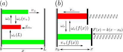
Figure 1: (a): Schematic representation of the confinement and possible MT configurations. From top to bottom: A MT growing with $v_{+}$; MT shrinks with $v_{-}$. MT in a state of growth and stuck to the boundary wall with $v_{+}=0$ and $\omega_{c,L}$. (b): Schematic representation of a single MT growing against the elastic obstacle. From top to bottom: MT shrinks with $v_{-}$. MT under force $F(x)=k\left(x-x_{0}\right)$ with $f(x)\equiv F(x)/F_{0}$, $v_{+}[f(x)]$, and force-dependent catastrophe rate $\omega_{c}[f(x)]$.

A single MT is confined to a one-dimensional box of fixed length $L$ with rigid boundary walls at $x=0$ and $x=L$ as shown schematically in Fig. 1(a) Holy1994 ; Dogt1998PRL . There is no force acting on the MT but within the box catastrophes are induced upon hitting the rigid walls. We propose the following mechanism for these wall-induced catastrophes: When the MT hits the boundary at $x=L$, its growth velocity $v_{+}$ has to reduce to zero, which leads to an increase of the catastrophe rate to $\omega_{c,L}\equiv\omega_{c}(v_{+}=0)$. Since $\omega_{c,L}$ is finite, wall-induced catastrophes are not instantaneous but the MT sticks for an average time $1/\omega_{c,L}$ to the boundary before the catastrophe, which is in contrast to previous studies Gov1993 . For the average time spent at the boundary before a catastrophe, we find $\omega_{c,L}^{-1}\approx 0.29\,{\rm s}$. The catastrophe rate at the wall, $\omega_{c,L}$, is much higher than the bulk catastrophe rate $\omega_{c}(v_{+})$. For $\omega_{\text{on}}=50\,{\rm s^{-1}}$ we find $\omega_{c,L}/\omega_{c}\simeq 2300$.

To include the mechanism of wall-induced catastrophes into the description by master equations, we introduce the probabilities $Q_{+}$ and $Q_{-}$ of finding the MT stuck to the boundary in a growing state and in a shrinking state, respectively. The stochastic time evolution of $Q_{+}(t)$ and $Q_{-}(t)$ is given by:

$$\partial_{t}Q_{+}(t) =-\omega_{c,L}Q_{+}(t)+\omega_{r}Q_{-}(t)+v_{+}p_{+}(L)$$ (16)

$$\partial_{t}Q_{-}(t) =+\omega_{c,L}Q_{+}(t)-\omega_{r}Q_{-}(t)-\frac{v_{-}}{\Delta}Q_{-}(t).$$ (17)

The quantity $v_{+}p_{+}(L)$ is the flow of probability from the interior of the confining box onto its boundary and is given by the solution of eq. (1) and (2) for $x=L$, while $(v_{-}/\Delta)Q_{-}$ is the probability current from the boundary back into the interior, where $\Delta$ denotes a small interval in which the flow $v_{-}Q_{-}$ can be measured. This implies that there is a boundary condition $v_{-}p_{-}(L,t)=(v_{-}/\Delta)Q_{-}$ for the backward current density at $x=L$, in addition to the reflecting boundary condition (3) at $x=0$. An identical model for wall-induced catastrophes has been introduced in Ref. Mulder2012 recently.

In the steady state and in the limit $\Delta\approx 0$ we find

$$Q_{+} \approx\frac{v_{+}}{\omega_{c,L}}p_{+}(L)$$ (18)

$$Q_{-} \approx 0,$$ (19)

and $v_{-}p_{-}(L,t)=(v_{-}/\Delta)Q_{-}=v_{+}p_{+}(L)$. Eq. (18) shows that there is a non-zero probability $Q_{+}$ of finding a MT in a state of growth and stuck to the boundary, which is given by the flow of probability from the interior of the confining box onto its boundary divided by the average time being stuck to the boundary. In contrast, eq. (19) states that there is no MT in a shrinking state and stuck to the wall. This is intuitively clear since a MT undergoing a catastrophe begins to shrink instantaneously. In the steady state, we solve eqs. (1), (2) and (18) simultaneously with the additional normalization $\int^{L}_{0}(p_{+}(x)+p_{-}(x))dx+Q_{+}=1$. We find $v_{+}p_{+}(x)=v_{-}p_{-}(x)$ and

$$P(x) =Ne^{x/\lambda}\left(1+\frac{v_{+}}{v_{-}}\right)$$ (20)

$$Q_{+} =N\frac{v_{+}}{\omega_{c,L}}e^{L/\lambda}$$ (21)

with $\lambda$ from eq. (4) and a normalization

$$N^{-1}=\lambda\left(1+\frac{v_{+}}{v_{-}}\right)\left(e^{L/\lambda}-1\right)+\frac{v_{+}}{\omega_{c,L}}e^{L/\lambda}.$$ (22)

Equation (20) shows that we find an exponential OPDF $P(x)$ in confinement with the same characteristic length $|\lambda|$. If the growth is unbounded in the absence of confinement, which corresponds to $\lambda^{-1}>0$, the OPDF is exponentially increasing; if the growth is bounded in the absence of confinement, which corresponds to $\lambda^{-1}<0$, the OPDF remains exponentially decreasing in confinement. The same result has been obtained in Ref. Gov1993 within a discrete growth model. In independent in vivo experiments, both exponentially increasing Komarova2002 and exponentially decreasing OPDFs Verd1992 have been found.

In the following we focus on the case $\lambda^{-1}>0$ of exponentially increasing OPDFs. In the steady state, the average length of a MT within the confining box is given by

$$\langle x\rangle =\int^{L}_{0}xP(x)dx+Q_{+}L$$

$$=N\left\{\left(1+\frac{v_{+}}{v_{-}}\right)\lambda^{2}\left[1+e^{L/\lambda}\left(\frac{L}{\lambda}-1\right)\right]\right.$$

$$~{}~{}~{}~{}~{}\left.+L\frac{v_{+}}{\omega_{c,L}}e^{L/\lambda}\right\}.$$ (23)

In the limit of instantaneous wall-induced catastrophes, $Q_{+}\approx 0$, we obtain

$$\frac{\langle x\rangle}{L}\approx\frac{1}{1-e^{-L/\lambda}}-\frac{\lambda}{L},$$ (24)

i.e., the average MT length $\langle x\rangle/L$ depends on the two control parameters $\omega_{r}$ and $\omega_{\text{on}}$ only via the ratio $L/\lambda$. This scaling property is lost if wall-induced catastrophes are not instantaneous because eq. (23) then exhibits additional $v_{+}$- and thus $\omega_{\text{on}}$-dependencies. Within our model the increased catastrophe rate at the boundary gives rise to an increased overall average catastrophe rate

$$\omega_{\text{c,eff}}=\omega_{c}(v_{+})+Q_{+}(\omega_{c,L}-\omega_{c}(v_{+})),$$ (25)

for which we find $\omega_{\text{c,eff}}\simeq 0.03\,{\rm s^{-1}}$ for $L=1\,{\rm\mu m}$ and $\omega_{\text{c,eff}}\simeq 0.006\,{\rm s^{-1}}$ for $L=10\,{\rm\mu m}$ as compared to $\omega_{c}\simeq 0.0015\,{\rm s^{-1}}$ for these conditions.

We set the length of the confining box to $L=1\,{\rm\mu m}$ and $L=10\,{\rm\mu m}$, which are typical length scales in experiments Faiv2008 ; Schek2007 and cellular environments daga2006 , and we calculate $\langle x\rangle$ and $Q_{+}$ as functions of $\omega_{\text{on}}$ and $\omega_{r}$. The parameter regimes displayed in Figs. 2 and 3 correspond to regimes $L/\lambda\gg 1$ for $L=10\,{\rm\mu m}$ and $L/\lambda\ll 1$ for $L=1\,{\rm\mu m}$. Results obtained from stochastic simulations agree with analytical findings (Figs. 2 and 3). It is clearly visible that the size $L$ of the confinement has a significant influence on $\langle x\rangle$, mainly via the ratio $L/\lambda$.

The probability $Q_{+}$ to find the MT at the wall increases with increasing rates in the range of $Q_{+}\approx 0,...,0.03$ and exhibits only a weak dependency on $L$, see Figs. 3. Even for maximum rates, the probability of finding a MT in a growing state and stuck to the wall is limited to several percent, due to the large catastrophe rate $\omega_{c,L}$ at $x=L$. Therefore, in most cases wall-induced catastrophes can be viewed as instantaneous, and the approximation (24) works well. For increasing on-rate $\omega_{\text{on}}$ or rescue rate $\omega_{r}$, the ratio $L/\lambda$ approaches $L/\lambda\approx L\omega_{r}/v_{-}$ from below. According to the approximation (24), the mean length $\langle x\rangle$ then increases and approaches $\langle x\rangle/L\approx{1}/{(1-e^{-L\omega_{r}/v_{-}})}-{v_{-}}/{L\omega_{r}}$ from below. For $L=10\,{\rm\mu m}$, we have $L/\lambda\gg 1$ and the length distribution is exponential, $P(x)\sim e^{x/\lambda}$. The ratio $\langle x\rangle/L$ saturates at a high value $\langle x\rangle/L\approx 0.7,...,0.9$ (Figs. 2 (a),(c)). For $L/\lambda\gg 1$ the MT length distribution becomes very narrow around the maximal length $L$. In contrast, for $L=1\,{\rm\mu m}$, we have $L/\lambda\ll 1$, and $L$ is too small to establish the characteristic exponential decay of the length distribution. The length distribution $P(x)$ is almost uniform, and the ratio $\langle x\rangle/L\approx 0.5,...,0.6$ deviates only slightly from the result $\langle x\rangle/L=1/2$ characteristic for a broad uniform distribution (Figs. 2(b),(d)).

Figure 2: The average length $\langle x\rangle$ as a function of $\omega_{\text{on}}$ and $\omega_{r}$ for confinement by fixed rigid walls. Data points are results from stochastic simulations, lines are analytical results (23). Top row: The average length $\langle x\rangle$ as a function of $\omega_{\text{on}}$ for different values of $\omega_{r}=0.03\,{\rm s}^{-1}(\boxdot),0.05\,{\rm s}^{-1}(\blacksquare),0.1\,{\rm s}^{-1}(\odot),0.2\,{\rm s}^{-1}(\bullet)$ and $0.3\,{\rm s}^{-1}(\triangle)$. (a) $L=10\,{\rm\mu m}$. (b) $L=1\,{\rm\mu m}$. Lower row: The average length $\langle x\rangle$ as a function of $\omega_{r}$ for different values of $\omega_{\text{on}}=25\,{\rm s}^{-1}(\blacksquare),50\,{\rm s}^{-1}(\boxdot),75\,{\rm s}^{-1}(\blacktriangle),100\,{\rm s}^{-1}(\boxdot)$. (c) $L=10\,{\rm\mu m}$. (d) $L=1\,{\rm\mu m}$.

Figure 3: The probability $Q_{+}$ to find the MT at the wall as a function of $\omega_{\text{on}}$ and $\omega_{r}$ for confinement by fixed rigid walls. Data points are results from stochastic simulations, lines are analytical results (18). Top row: $Q_{+}$ as a function of $\omega_{\text{on}}$ for different values of $\omega_{r}=0.03\,{\rm s}^{-1}(\boxdot),0.05\,{\rm s}^{-1}(\blacksquare),0.1\,{\rm s}^{-1}(\odot),0.2\,{\rm s}^{-1}(\bullet)$ and $0.3\,{\rm s}^{-1}(\triangle)$. (a) $L=10\,{\rm\mu m}$. (b) $L=1\,{\rm\mu m}$.
Lower row: $Q_{+}$ as a function of $\omega_{r}$ for different values of $\omega_{\text{on}}=25\,{\rm s}^{-1}(\blacksquare),50\,{\rm s}^{-1}(\boxdot),75\,{\rm s}^{-1}(\blacktriangle),100\,{\rm s}^{-1}(\boxdot)$. (c) $L=10\,{\rm\mu m}$. (d) $L=1\,{\rm\mu m}$.

V Constant force

In the second scenario a constant force $F$ is applied to the MT and the right boundary is removed, so that the MT is allowed to grow on $x\in[0,\infty[$. According to eq. (13) the growth velocity under force is smaller, but it remains constant for fixed $f$. With eq. (10) this results in a higher, but also constant, catastrophe rate $\omega_{c}[v_{+}(f)]>\omega_{c}[v_{+}(0)]$. Since $v_{-}$ and $\omega_{r}$ are independent of force, the stochastic dynamics of the MT is described by eq. (1) and (2) with the same solutions $P(x,t)$ as in the absence of force, but with a decreased velocity of growth $v_{+}(f)$ and an increased catastrophe rate $\omega_{c}(f)$ Dogt1993PRL ; Verd1992 . In particular, we still find two regimes, a regime of bounded growth and a regime of unbounded growth.

In the regime of bounded growth $P(x,t)$ is again exponentially decreasing, and the force-dependent average length is $\langle x(f)\rangle=|\lambda(f)|$ with the corresponding force-dependent length parameter

$$\lambda(f)\equiv\frac{v_{+}(f)v_{-}}{v_{+}(f)\omega_{r}-v_{-}\omega_{c}(f)}$$ (26)

as compared to eq. (4) in the absence of force. In the regime of unbounded growth $\langle x(f)\rangle$ increases linearly in time with the force-dependent mean velocity $J(f)=[v_{+}(f)\omega_{r}-v_{-}\omega_{c}(f)]/[\omega_{r}+\omega_{c}(f)]$, cf. eq. (7). The MT length distribution $P(x,t)$ assumes again a Gaussian form (6) where also the diffusion constant $D_{J}(f)$ follows the same eq. (8) with force-dependent growth velocity $v_{+}(f)$ and catastrophe rate $\omega_{c}(f)$.

In the presence of a constant force $f$, the transition between bounded and unbounded growth is governed by the force-dependent parameter $\lambda(f)$. The regimes of bounded and unbounded growth are now separated by the condition $\lambda^{-1}(f)=0$, which is shifted compared to the case $f=0$, see Fig. 4(a). The inverse length parameter $\lambda^{-1}(f)$ is a monotonously decreasing function of force $f$ and changes sign from positive to negative values for increasing force $f$. Therefore $\lambda^{-1}(f_{c})=0$ or

$$v_{+}(f_{c})\omega_{r}=v_{-}\omega_{c}(f_{c}),$$ (27)

defines a critical force for the transition from unbounded to bounded growth. A single MT exhibiting unbounded growth ($\lambda^{-1}(0)>0$) in the absence of force undergoes a transition to bounded growth with $\lambda^{-1}(f)<0$ by applying a supercritical force $f>f_{c}$. On the other hand, starting with a combination of on-rate $\omega_{\text{on}}$ and rescue rate $\omega_{r}$ and a force $f$, which results in bounded growth with $\lambda^{-1}(f)<0$, the MT can still enter the regime of unbounded growth by increasing $\omega_{\text{on}}$ or $\omega_{r}$ so that the force $f$ becomes subcritical, $\lambda^{-1}(f)>0$ or $f<f_{c}$.

Rewriting condition (27) as $v_{+}(f_{c})=v_{-}\omega_{c}(f_{c})/\omega_{r}>0$ and using that $v_{+}(f)$ decreases with $f$, it follows that the critical force is always smaller than the stall force, $f_{c}<f_{\text{stall}}$, which satisfies $v_{+}(f_{\text{stall}})=0$, and it approaches the stall force only for vanishing catastrophe rate. Qualitatively, we can obtain an explicit result for the critical force $f_{c}$ by using the approximations of an exponentially decreasing growth velocity, $v_{+}(f)\approx v_{+}(0)e^{-f}$, which is valid for $\omega_{\text{on}}\gg\omega_{\text{off}}$ (see eq. (13)), and an exponentially increasing catastrophe rate above the characteristic force $F_{0}$, eq. (15), in the condition (27) for the critical force. This leads to

$$f_{c}\sim\frac{1}{2}\ln\left(\frac{v_{+}(0)\omega_{r}}{v_{-}\omega_{c}(0)}\right)\sim\frac{1}{2}\ln\left(\frac{\omega_{\text{on}}d\omega_{r}}{v_{-}\omega_{c}(0)}\right)$$ (28)

which shows that the critical force grows approximately logarithmically with on-rate $\omega_{\text{on}}$ (note that the catastrophe rate in the absence of force decreases with $\omega_{\text{on}}$ as $\omega_{c}(0)\propto 1/\omega_{\text{on}}$ Flyv1996PRE ) and rescue rate $\omega_{r}$. A negative $f_{c}$ for small on-rates and rescue rates signals that the MT is for all forces $f>0$ in the bound phase. In Fig. 4(b) we show exact results for the critical force $f_{c}$ as a function of the on-rate $\omega_{\text{on}}$ and for different rescue rates $\omega_{r}$ from solving condition (28) numerically and from stochastic simulations. Agreement between both methods is good.

The condition $\lambda^{-1}(f)=0$ specifies the boundary between bounded and unbounded growth at a given force $f$. In Fig. 4(a), the resulting phase boundary is shown as a function of $\omega_{\text{on}}$ and $\omega_{r}$. There is good agreement between numerical solutions of $\lambda^{-1}(f)=0$ and stochastic simulations. With increasing force, the boundary between the two regimes of growth shifts to higher values of $\omega_{\text{on}}$ and $\omega_{r}$, and forces up to $F\sim 1.4\cdot F_{0}$ can be overcome by a single MT in the parameter regimes of $\omega_{\text{on}}$ and $\omega_{r}$ considered.

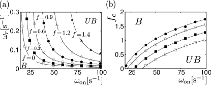
Figure 4: (a): Phase boundary between bounded (B) and unbounded growth (UB) as a function of $\omega_{\text{on}}$ and $\omega_{r}$ for MT growth under constant force. Data points for $f=0(\boxdot),0.3(\blacksquare),0.6(\odot),0.9(\bullet),1.2(\triangle),1.4(\blacktriangle)$ represent results from simulations, lines represent solutions of $v_{+}(f)\omega_{r}=v_{-}\omega_{c}(f)$ for a constant force $f$. (b): Critical force $f_{c}$ as a function of $\omega_{\text{on}}$ for $\omega_{r}=0.03\,{\rm s}^{-1}(\boxdot),0.05\,{\rm s}^{-1}(\blacksquare),0.1\,{\rm s}^{-1}(\odot),0.2\,{\rm s}^{-1}(\bullet)$. Data points represent results from simulations, lines represent the solution of eq. (27) for a fixed combination of $\omega_{\text{on}}$ and $\omega_{r}$.

VI Elastic force

In the third scenario, an elastically coupled barrier is placed in front of the MT as shown in Fig. 1(b), which models the optical traps used in Refs. Schek2007 ; Laan2008 or the elastic cell cortex in vivo. If the barrier is displaced from its equilibrium position $x_{0}$ by the growing MT with length $x>x_{0}$, it causes a force $F(x)=k(x-x_{0})$ resisting further growth. For $x<x_{0}$ there is no force. We use $x_{0}=0\,{\rm\mu m}$ in the case of vanishing rescue rate and $x_{0}=10\,{\rm\mu m}$ in the case of finite rescue rate and a spring constant $k$ in the range $10^{-7}\,{\rm N/m}$ (soft) to $10^{-5}\,{\rm N/m}$ (stiff as in the optical trap experiments in Laan2008 ).

An elastic force $F(x)=k(x-x_{0})$ represents the simplest and most generic $x$-dependent force. Whereas for a confinement of fixed length or a constant force, the MT length $x$ was the only stochastic variable, the force $F(x)$ itself is now coupled to $x$ and becomes stochastic as well. Therefore, not only are the MT length distributions of interest but also the maximal and average polymerization forces which are generated during MT growth.

VI.1 Vanishing rescue rate

We first discuss growth in the absence of rescue events, $\omega_{r}=0$. This situation corresponds to optical trap experiments Schek2007 ; Laan2008 , which are performed on short time scales and no rescue events are observed. In a state of growth the MT grows against the elastic obstacle with velocity $v_{+}[f(x)]$ and $f(x)$ increases. For simplicity we suppress the $x$-dependency in the notation in the following. At a maximal polymerization force $f_{\text{max}}$, the MT undergoes a catastrophe and starts to shrink back to zero and the dynamics stop due to missing rescue events. No steady state is reached. Since switching to the state of shrinkage is a stochastic process, the maximal polymerization force $f_{\text{max}}$ is a stochastic quantity which fluctuates around its average value. We calculate the average maximal polymerization force $\langle f_{\text{max}}\rangle$ within a mean field approach. Here $\langle...\rangle$ denotes an ensemble average over many realizations of the growth experiment.

Because no steady state is reached in the absence of rescue events, we have to use a dynamical mean field approach, which is based on the fact that the MT growth velocity $dx/dt=v_{+}(f)$ is related to the time evolution of the force by $df/dt=(k/F_{0})dx/dt$. In mean field theory, this results in the following equation of motion for $\langle f\rangle$,

$$\frac{d}{dt}\langle f\rangle=\frac{k}{F_{0}}v_{+}(\langle f\rangle),$$ (29)

where we used the mean field approximation $\langle v_{+}(f)\rangle\approx v_{+}(\langle f\rangle)$. With the initial condition $\langle f\rangle(0)=0$ we find a time evolution

$$\langle f\rangle(t) = \ln\left[\left(1-\omega_{\text{on}}/\omega_{\text{off}}\right)e^{-t/\tau}+\omega_{\text{on}}/\omega_{\text{off}}\right]$$ (30)

$$\approx f_{\text{stall}}+\ln\left[1-\exp(-t/\tau)\right]$$ (31)

with a characteristic time scale $\tau=F_{0}/dk\omega_{\text{off}}\approx 10^{2}...10^{4}\,{\rm s}$ for $k\approx 10^{-5}...10^{-7}\,{\rm N/m}$. For long times $t\gg\tau$, eq. (30) approaches the dimensionless stall force $\langle f\rangle=f_{\text{stall}}$, see eq. (14), which is the maximal polymerization force in the absence of catastrophes. The approximation (31) holds for $\omega_{\text{on}}/\omega_{\text{off}}\gg 1$.

MT growth is ended, however, by a catastrophe, and the average time spent in the growing state is $t=1/\omega_{c}(\langle f_{\text{max}}\rangle)$. Together with eq. (30), this gives a self-consistent mean field equation for the maximal polymerization force $\langle f_{\text{max}}\rangle$,

$$\langle f_{\text{max}}\rangle=\ln\left[\left(1-\omega_{\text{on}}/\omega_{\text{off}}\right)e^{-1/\omega_{c}(\langle f_{\text{max}}\rangle)\tau}+\omega_{\text{on}}/\omega_{\text{off}}\right].$$ (32)

The maximal polymerization force $\langle f_{\text{max}}\rangle$ is always smaller than the stall force $f_{\text{stall}}$ as can be seen from eqs. (30,31). Since $\omega_{\text{on}}/\omega_{\text{off}}\gg\omega_{c}\tau\gg 1$ for realistic force and parameter values, eq. (32) can be approximated by

$$\langle f_{\text{max}}\rangle \approx \ln\left(\frac{\omega_{\text{on}}}{\omega_{\text{off}}\tau\omega_{c}(\langle f_{\text{max}}\rangle)}\right)$$ (33)

$$= f_{\text{stall}}-\ln\left[\tau\omega_{c}(\langle f_{\text{max}}\rangle)\right].$$

For a catastrophe rate increasing exponentially above the characteristic force $F_{0}$, eq. (15), we find

$$\langle f_{\text{max}}\rangle\sim\frac{1}{2}\ln\left(\frac{\omega_{\text{on}}dk}{F_{0}\omega_{c}(0)}\right),$$ (34)

i.e., the maximal polymerization force grows logarithmically in $\omega_{\text{on}}$ (note that the catastrophe rate in the absence of force decreases as $\omega_{c}(0)\propto 1/\omega_{\text{on}}$ Flyv1996PRE ), see Fig. 5 for $k=10^{-5}\,{\rm N/m}$. Within a slightly different catastrophe model obtained from experimental data and discussed in section VII, this logarithmic dependence can be shown exactly.

Fig. 5 shows $\langle f_{\text{max}}\rangle$ as a function of $\omega_{\text{on}}$. Analytical results from eq. (32) agree with numerical findings from stochastic simulations. The maximal polymerization force $\langle f_{\text{max}}\rangle$ increases with increasing $k$, see eq. (34), but it remains smaller than the stall force $f_{\text{stall}}$. Stochastic simulations show considerable fluctuations of $f_{\text{max}}$, which are caused by broad and exponentially decaying probability distributions for $f_{\text{max}}$ and which we quantify by measuring the standard deviation $\langle f_{\text{max}}^{2}\rangle-\langle f_{\text{max}}\rangle^{2}$. For increasing $k$, probability distributions become more narrow and mean field results approach the simulation results for $\langle f_{\text{max}}\rangle$.

Figure 5: Average maximal polymerization force $\langle f_{\text{max}}\rangle$ for an elastic obstacle and in the absence of rescues as a function of $\omega_{\text{on}}$ for different values of $k=10^{-5}\,{\rm N/m}(\blacktriangle)$, $10^{-6}\,{\rm N/m}(\blacksquare)$ and $10^{-7}\,{\rm N/m}(\bullet)$. Data points represent results from simulations, solid lines are solutions of eq. (32). Error bars represent the standard deviation of the stochastic quantity $\langle f_{\text{max}}\rangle$. Dashed line: dimensionless stall force $f_{\text{stall}}=\ln\left(\omega_{\text{on}}/\omega_{\text{off}}\right)$.

VI.2 Non-zero rescue rate

For a non-zero rescue rate $\omega_{r}$, phases of growth, in which $f(x)$ increases and which last $1/\omega_{c}(f)$ on average, are ended by catastrophes which are followed by phases of shrinkage. Shrinking phases last $1/\omega_{r}$ on average, and during shrinkage the elastic obstacle is relaxed and $f(x)$ decreases. After rescue, the MT switches back to a state of growth. In contrast to the case without rescue events, the system can attain a steady state. In this steady state, the average length loss during shrinkage, $v_{-}/\omega_{r}$, equals the average length gain during growth, $v_{+}(f)/\omega_{c}(f)$, and the MT oscillates around a time-averaged stall length $\langle x\rangle$, which is directly related to the time-averaged polymerization force by $\langle f\rangle=(k/F_{0})(\langle x\rangle-x_{0})$. In the following, the steady state dynamics and the average polymerization force are characterized. We start with an analysis of the full master equations focusing on the stationary state followed by a dynamical mean field theory, which can also be applied to dilution experiments.

In the presence of a $x$-dependent force $f(x)$, the master equations for the time evolution of $p_{+,-}(x,t)$ become

$$\partial_{t}p_{+}(x,t) =-\omega_{c}(x)p_{+}(x,t)+\omega_{r}p_{-}(x,t)$$

$$~{}~{}~{}~{}~{}~{}~{}~{}~{}~{}~{}~{}~{}~{}~{}~{}~{}~{}~{}-\partial_{x}(v_{+}(x)p_{+}(x,t))$$ (35)

$$\partial_{t}p_{-}(x,t) =\omega_{c}(x)p_{+}(x,t)-\omega_{r}p_{-}(x,t)+v_{-}\partial_{x}p_{-}(x,t),$$ (36)

which differ from eqs. (1) and (2) by the $x$-dependence of growth velocity and catastrophe rate. Both growth velocity $v_{+}(x)=v_{+}[f(x)]$ and catastrophe rate $\omega_{c}(x)=\omega_{c}\{v_{+}[f(x)]\}$ become $x$-dependent via their force-dependence. Therefore, also the force-dependent length parameter $\lambda(f)$ from eq. (26) becomes $x$-dependent via its force-dependence, $\lambda(x)=\lambda[f(x)]$. Eqs.  (1) and (2) are supplemented by reflecting boundary conditions $v_{+}(0)p_{+}(0,t)=v_{-}p_{-}(0,t)$ at $x=0$, similar to eq. (3).

For the steady state, eqs. (35) and (36) are solved on the half-space $x>0$ with reflecting boundary conditions at $x=0$, and we can calculate the overall MT length distribution $P(x)=p_{+}(x)+p_{-}(x)$ explicitly,

$$P(x)=N\left(1+\frac{v_{-}}{v_{+}(x)}\right)e^{x_{0}/\lambda(0)}\exp\left[\int^{x}_{x_{0}}dx^{\prime}/\lambda(x^{\prime})\right]$$ (37)

with a normalization

$$N^{-1}=\int_{0}^{\infty}dx\left(1+\frac{v_{-}}{v_{+}(x)}\right)e^{x_{0}/\lambda(0)}e^{\int^{x}_{x_{0}}dx^{\prime}/\lambda(x^{\prime})},$$ (38)

where $\lambda(x)=\lambda(f\!=\!0)$ in the force-free region $x<x_{0}$ and $\lambda(x)=\lambda[f(x)]$ for $x>x_{0}$ and, likewise, $v_{+}(x)=v_{+}(f\!=\!0)$ for $x<x_{0}$ and $v_{+}(x)=v_{+}[f(x)]$ for $x>x_{0}$. This implies $e^{x_{0}/\lambda(0)}e^{\int^{x}_{x_{0}}dx^{\prime}/\lambda(x^{\prime})}=e^{x/\lambda(0)}$ and, thus, a simple exponential dependence of $P(x)$ for $x<x_{0}$. A similar OPDF has been found for dynamic MTs in the presence of MT end-tracking molecular motors Tischer2010 .

With increasing length $x$, also the force $f(x)$ increases and, thus, $v_{+}[f(x)]$ decreases and $\omega_{c}[f(x)]$ grows exponentially. If $x$ becomes sufficiently large that the condition $\lambda^{-1}[f(x)]<0$ holds, the distribution $P(x)$ starts to decrease exponentially. In this length regime the MT undergoes a catastrophe with high probability. Because the distribution always decreases exponentially for sufficiently large $x$, a single MT growing against an elastic obstacle is always in the regime of bounded growth regardless of how large the values of $\omega_{\text{on}}$ and $\omega_{r}$ are chosen. This behavior is a result of the linearly increasing force, which gives rise to arbitrarily large forces for increasing $x$ in contrast to growth under constant or zero force, where a MT can either be in a phase of bounded or unbounded growth as mentioned above.

The behavior is also in contrast to length distributions in confinement between fixed rigid walls, where we found a transition between exponentially decreasing and increasing length distributions: The elastic obstacle typically leads to a non-monotonic length distribution with a maximum in the region $x>x_{0}$. (as long as the on-rate $\omega_{\text{on}}$ and rescue rate $\omega_{r}$ are sufficiently large and the obstacle stiffness $k$ sufficiently small). While rescue events (and an exponential decrease in the growth velocity $v_{+}[f(x)]$) cause $P(x)$ to increase exponentially for small MT length, catastrophes are responsible for an exponential decrease for large $x$. The interplay between rescues and catastrophes gives rise to strongly localized probability distributions with a maximum. Figs. 6 (a-d) show the steady state distribution $P(x)$ obtained from eq. (37) for different values of $\omega_{\text{on}}$ and $\omega_{r}$. We chose $k=10^{-7}\,{\rm N/m}$ and $x_{0}=10\,{\rm\mu m}$. In the steady state, a stable length distribution with a well defined average length $\langle x\rangle=\int_{0}^{\infty}P(x)xdx$ is maintained although the MT is still subject to dynamic instability. The length distributions drop to zero for large $x$, where $\lambda^{-1}(x)\!\sim\!-\omega_{c}(x)/v_{+}(x)$ and $\omega_{c}(x)/v_{+}(x)$ increases exponentially with increasing force.

The most probable MT length $x_{mp}$ maximizes the stationary length distribution (37). Because $v_{-}\gg v_{+}(x)$ and using the approximation of an exponentially decreasing growth velocity, $v_{+}[f(x)]\approx v_{+}(0)e^{-f(x)}$, which is valid for $\omega_{\text{on}}\gg\omega_{\text{off}}$ (see eq. (13)), we obtain a condition $\lambda^{-1}(x_{mp})=-\partial_{x}f(x_{mp})=-k/F_{0}$ or

$$v_{+}(f_{mp})\omega_{r}-v_{-}\omega_{c}(f_{mp})=-(k/F_{0})v_{-}v_{+}(f_{mp})$$ (39)

for the corresponding most probable force $f_{mp}=(k/F_{0})(x_{mp}-x_{0})$.

For an exponentially increasing catastrophe rate above the characteristic force $F_{0}$, eq. (15), we find

$$f_{mp}\sim\frac{1}{2}\ln\left[\frac{v_{+}(0)\omega_{r}}{v_{-}\omega_{c}(0)}\left(1+\frac{kv_{-}}{F_{0}\omega_{r}}\right)\right]$$ (40)

We can distinguish two limits: (i) For a soft obstacle with $kv_{-}/F_{0}\omega_{r}\ll 1$ the most probable force $f_{mp}$ is identical to the critical force $f_{c}$ for MT dynamics under constant force, see (28), because the right hand side in the condition (39) for $f_{mp}$ can be neglected and we exactly recover condition (27) for $f_{c}$. The most probable MT length thus “self-organizes” into a “critical” state with $f_{mp}\approx f_{c}$, and a MT pushing against a soft elastic obstacle generates the same force as if growing against a constant force. This force grows logarithmically in the on-rate $\omega_{\text{on}}$ and the rescue rate $\omega_{r}$. (ii) For a stiff obstacle with $kv_{-}/F_{0}\omega_{r}\gg 1$, on the other hand, the most probable force is larger than the critical force, $f_{mp}\gg f_{c}$, and the MT growing against a stiff obstacle generates a higher force. This limit can also be realized for vanishing rescue rate $\omega_{r}$, and for $kv_{-}/F_{0}\omega_{r}\gg 1$ we indeed recover the maximal pushing force in the absence of rescue events, i.e.  $f_{mp}\approx\langle f_{\text{max}}\rangle$ from eq. (34) with $v_{+}(0)\approx\omega_{\text{on}}d$. This force grows logarithmically in the on-rate $\omega_{\text{on}}$. Furthermore, if $f_{mp}$ becomes negative for small on-rates and rescue rates (leading to $\lambda^{-1}(0)<-k/F_{0}$, see eq. (40)) the stationary length distribution has no maximum, see for example Figs. 6(a,b) at the lowest on-rates.

With respect to the MT’s ability to generate force the two limits can be interpreted also in the following way: $F_{0}$ is the characteristic force above which the catastrophe rate increases exponentially. For $kv_{-}/F_{0}\omega_{r}\ll 1$, the average length loss during a period of shrinkage, $v_{-}/\omega_{r}$, is much smaller than the length $F_{0}/k$, which is the displacement $x-x_{0}$ of the elastic obstacle under the characteristic force $F_{0}$. Therefore, the MT tip always remains in the region $x>x_{0}$ under the influence of the force for a soft obstacle with $kv_{-}/F_{0}\omega_{r}\ll 1$, whereas it typically shrinks back into the force-free region $x<x_{0}$ before the next rescue event for a stiff obstacle $kv_{-}/F_{0}\omega_{r}\gg 1$. The force generation by the MT can only be enhanced by rescue events if rescue takes place under force in the regime $x>x_{0}$. Therefore, we find an increased polymerization force $f_{mp}\approx f_{c}\gg\langle f_{\text{max}}\rangle$ as compared to the force $f_{\text{max}}$ without rescue events discussed in the previous section only in the limit $kv_{-}/F_{0}\omega_{r}\ll 1$, i.e., for a soft obstacle or sufficiently large rescue rate. In the limit $kv_{-}/F_{0}\omega_{r}\gg 1$ of a stiff obstacle, the MT only generates the same force as in the absence of rescues, $f_{mp}\approx\langle f_{\text{max}}\rangle$.

By comparing the condition (27) or $v_{+}(f_{c})=v_{-}\omega_{c}(f_{c})/\omega_{r}$ for the critical force $f_{c}$, the condition (39) or $v_{+}(f_{mp})=v_{-}\omega_{c}(f_{mp})/\omega_{r}(1+kv_{-}/F_{0})<v_{-}\omega_{c}(f_{mp})/\omega_{r}$ for the most probable force $f_{mp}$, and the condition $v_{+}(f_{\text{stall}})=0$ for the stall force, see eq. (14), it follows that

$$f_{c}\leq f_{mp}\ll f_{\text{stall}}$$ (41)

i.e., force generated against an elastic obstacle is between critical and stall force but typically well below the stall force, which is the maximal polymerization force in the absence of catastrophes. Therefore, the stall length $x_{\rm stall}=(F_{0}/k)\ln\left(\omega_{\text{on}}/\omega_{\text{off}}\right)+x_{0}$ is always much larger than the most probable MT length $x_{mp}$ at the maximum of the stationary length distribution, see Fig. 6(a). This shows that the dynamic instability reduces the typical MT length significantly compared to simple polymerization kinetics.

In order to quantify the width of the stationary distribution $P(x)$ we expand the exponential in (37) up to second order about the maximum at $x_{mp}$. To do so we first expand $\lambda^{-1}(x)$ up to first order:

$$\lambda^{-1}(x)\approx-\frac{k}{F_{0}}\left[\frac{v_{+}(x_{mp})\omega_{r}+v_{-}\omega_{c}(x_{mp})}{v_{+}(x_{mp})v_{-}}\right]\left(x-x_{mp}\right)$$ (42)

where we used $v_{+}[f(x)]\approx v_{+}(0)e^{-f(x)}$, which is valid for $\omega_{\text{on}}\gg\omega_{\text{off}}$ (see eq. (13)), and where we approximated the catastrophe rate by an exponential $\omega_{c}[f(x)]\approx\omega_{c}(0)e^{f(x)}$ according to eq. (15) resulting in $\omega_{c}^{\prime}[f(x)]\approx k\omega_{c}[f(x)]/F_{0}$. The prime denotes a derivative with respect to the length $x$. Using the expansion (42) in eq. (37), we obtain an approximately Gaussian length distribution

$$P(x)\approx \ N\left(1+\frac{v_{-}}{v_{+}(x)}\right)e^{x_{0}/\lambda(0)}\ \times$$

$$\exp\left[\frac{(x_{mp}-x_{0})^{2}}{2\sigma^{2}}\right]\exp\left[-\frac{(x-x_{mp})^{2}}{2\sigma^{2}}\right]$$ (43)

with a width

$$\sigma^{2} = \frac{F_{0}}{k}\left[\frac{v_{+}(x_{mp})v_{-}}{v_{+}(x_{mp})\omega_{r}+v_{-}\omega_{c}(x_{mp})}\right]$$ (44)

$$\approx \left(\frac{F_{0}}{k}\right)^{2}\left(1+\frac{2F_{0}\omega_{r}}{kv_{-}}\right)^{-1}$$

where we used the saddle point condition (39) in the last approximation and the exponential approximations $v_{+}[f(x)]\approx v_{+}(0)e^{-f(x)}$ and $\omega_{c}[f(x)]\approx\omega_{c}(0)e^{f(x)}$. Again we have to distinguish the two limits of soft and stiff obstacles: (i) For a soft obstacle with $kv_{-}/F_{0}\omega_{r}\ll 1$ we find $\sigma^{2}\approx F_{0}v_{-}/2k\omega_{r}$. This shows that the width of the length distribution decreases with increasing $\omega_{r}$ but is roughly independent of the on-rate $\omega_{\text{on}}$, as can also be seen in the series of simulation results shown in Figs. 6. Closer inspection of the simulation results shows that the width of the stationary length distribution $P(x)$ is slightly decreasing with the on-rate $\omega_{\text{on}}$. (ii) For a stiff obstacle with $kv_{-}/F_{0}\omega_{r}\gg 1$, on the other hand, we find $\sigma^{2}\approx(F_{0}/k)^{2}$, which only depends on obstacle stiffness. All in all, $\sigma^{2}$ is monotonously decreasing for increasing stiffness $k$.

For a soft obstacle $kv_{-}/F_{0}\omega_{r}\ll 1$, high rescue rates thus lead to a sharply peaked length distribution $P(x)$ and suppress fluctuations of the MT length around $x=x_{mp}$ and we expect $\langle x\rangle\approx x_{mp}$ to a very good approximation. This property of a sharp maximum in $P(x)$ will make the mean field approximation that is discussed in the next section very accurate.

If the obstacle stiffness $k$ is increased the most probable MT length $x_{mp}=x_{0}+f_{mp}F_{0}/k$ approaches $x_{0}$, and a considerable probability weight is shifted to MT lengths $x$ below $x_{0}$ (see Fig. 6 (e)). The average length approaches and finally drops below $x_{0}$. This signals that the force generated by the MT is no longer sufficient to push the obstacle out of its equilibrium position $x_{0}$. The obstacle now serves as a fixed rigid boundary and $P(x)$ approaches the results eq. (21) and (22). The dynamics of a single MT within confinement can therefore be seen as a special case of the dynamics in the presence of an elastic obstacle, i.e., for small $\omega_{\text{on}}$ and $\omega_{r}$ or for large spring constants $k$.

Figure 6: Stationary MT length distribution $P(x)$ in the steady state for growth against an elastic obstacle with $\omega_{\text{on}}=25\,{\rm s}^{-1},50\,{\rm s}^{-1},75\,{\rm s}^{-1},100\,{\rm s}^{-1}$ and different values of $\omega_{r}$. We set $k=10^{-7}\,{\rm N/m}$ and $x_{0}=10^{-5}\,{\rm m}$. (a) $\omega_{r}=0.03\,{\rm s}^{-1}$. (b) $\omega_{r}=0.05\,{\rm s}^{-1}$. (c) $\omega_{r}=0.1\,{\rm s}^{-1}$. (d) $\omega_{r}=0.2\,{\rm s}^{-1}$. Dashed line represents $x_{0}$. In picture (a) the stall length $x_{s}$ for $\omega_{\text{on}}=25\,{\rm s}^{-1}$, obtained from simple polymerization kinetics, is indicated by an arrow. (e): $P(x)$ for $\omega_{\text{on}}=50\,{\rm s}^{-1}$, $\omega_{r}=0.05\,{\rm s}^{-1}$ and different values of the spring constant $k$.

So far we have quantified the generated force by the most probable force $f_{mp}$. The generated force can also be quantified by the average steady-state force $\langle f\rangle=\int^{\infty}_{0}f(x)P(x)dx$. Using the stationary distribution (37) with normalization (38) we can calculate $\langle f\rangle$; results are shown in Fig. 7 in comparison with the most probable force $f_{mp}$, which is determined numerically from the maximum of $P(x)$, and the stall force $f_{\text{stall}}$ in the absence of dynamic instability from eq. (14). For $\langle f\rangle$, there is excellent agreement with stochastic simulations over the complete range of parameter values. The results clearly show that the dynamic instability reduces the ability to generate polymerization forces since, even for large values of $\omega_{\text{on}}$ and $\omega_{r}$, the average force $\langle f\rangle$ is always smaller than the stall force. Nevertheless forces up to $F\sim 1.5\,F_{0}$ can be obtained in the steady state for realistic parameter values. Comparing $\langle f\rangle$ and $f_{mp}$ we find $\langle f\rangle\leq f_{mp}$, and both forces become identical, $\langle f\rangle\approx f_{mp}$, in the limit of large rescue rates or a soft obstacle $kv_{-}/F_{0}\omega_{r}\ll 1$, where also the length distributions $P(x)$ become sharply peaked, see Fig.  6. Comparing different combinations of $\omega_{\text{on}}$ and $\omega_{r}$ and the corresponding forces, one finds that the influence of the on-rate $\omega_{\text{on}}$ on force generation is more significant than the influence of the rescue rate $\omega_{r}$. For $\omega_{\text{on}}=100\,{\rm s}^{-1}$, a four fold increase of the rescue rate $\omega_{r}$ gives rise to an increase of $\langle f\rangle$ by a factor of $\sim 1.5$, while for $\omega_{r}=0.1\,{\rm s}^{-1}$, a four fold increase of the on-rate $\omega_{\text{on}}$ results in an amplification of the force $\langle f\rangle$ by a factor of $\sim 9$. These results can be explained within a mean field theory presented in the next section.

Figure 7: Average steady state force $\langle f\rangle$ as a function of $\omega_{\text{on}}$ for growth against an elastic obstacle with $\omega_{r}=0.03\,{\rm s}^{-1}(\boxdot),0.05\,{\rm s}^{-1}(\blacksquare),0.1\,{\rm s}^{-1}(\odot),0.2\,{\rm s}^{-1}(\bullet)$ and $k=10^{-7}\rm{N/m}$. Solid lines: $\langle f\rangle=\int^{\infty}_{0}f(x)P(x)dx$ with $P(x)$ given by eqs. (37) and (38). Dashed lines: $\langle f\rangle$ calculated from mean field equation (46). Dotted lines: most probable force $f_{mp}$, measured in simulations, for $\omega_{r}=0.03\,{\rm s}^{-1}$ and $\omega_{r}=0.05\,{\rm s}^{-1}$. Also shown is the dimensionless stall force $f_{\text{stall}}$ obtained from simple polymerization kinetics (14).

Figure 8: Average steady state force $\langle f\rangle$ as a function of $\omega_{\text{on}}$ for growth against an elastic obstacle with $\omega_{r}=0.03\,{\rm s}^{-1}(\boxdot),0.05\,{\rm s}^{-1}(\blacksquare),0.1\,{\rm s}^{-1}(\odot),0.2\,{\rm s}^{-1}(\bullet)$ and $k=10^{-5}\rm{N/m}$. Solid lines: $\langle f\rangle=\int^{\infty}_{0}f(x)P(x)dx$ with $P(x)$ given by eqs. (37) and (38). Dashed lines from bottom to top: $\langle f\rangle$ calculated from mean field equation (46) for $\omega_{r}=0.03\,{\rm s}^{-1},0.05\,{\rm s}^{-1},0.1\,{\rm s}^{-1}$ and $0.2\,{\rm s}^{-1}$.

VI.3 Mean field approach (non-zero rescue rate)

In the following, we show that we can reproduce many of the results for the average polymerization force $\langle f\rangle$ for non-zero rescue rate using a simplified mean field approach. Using the mean field approach, we can also address the time evolution of the average force $\langle f\rangle$, for example, in dilution experiments. Since the switching between the two states of growth is a stochastic process, the length $x$ and the force $f(x)$ are stochastic variables. Therefore, the velocity of growth $v_{+}[f(x)]$ and the catastrophe rate $\omega_{+}[f(x)]$ also become stochastic variables which, in the steady state, fluctuate around their average values. Within the mean field approach we neglect these fluctuations and use $\langle v_{+}[f(x)]\rangle=v_{+}(\langle f\rangle)$ and $\langle\omega_{+}[f(x)]\rangle=\omega_{+}(\langle f\rangle)$. In the mean field approximation, the average time in the growing state is given by $1/\omega_{c}(\langle f\rangle)$ and the average growth velocity is $v_{+}(\langle f\rangle)$. The average time in a shrinking state is $1/\omega_{r}$. Therefore, the mean field probabilities to find the MT growing or shrinking are $p_{+}=\omega_{r}/[\omega_{r}+\omega_{c}(\langle f\rangle)]$ and $p_{-}=\omega_{c}(\langle f\rangle)/[\omega_{r}+\omega_{c}(\langle f\rangle)]$, respectively. This results in the following mean field average velocity $v$ of a single MT under force:

$$v(\langle f\rangle)=\frac{v_{+}(\langle f\rangle)\omega_{r}-v_{-}\omega_{c}(\langle f\rangle)}{\omega_{r}+\omega_{c}(\langle f\rangle)}.$$ (45)

In the steady state the barrier is pushed so far that $\langle f\rangle$ stalls the MT. We require $v(\langle f\rangle)=0$ and obtain the condition

$$v_{+}(\langle f\rangle)\omega_{r}=v_{-}\omega_{c}(\langle f\rangle)$$ (46)

for the stationary state. This condition corresponds to a force, where the average length gain during growth, $v_{+}(\langle f\rangle)/\omega_{c}(\langle f\rangle)$, equals the average length loss during shrinking, $v_{-}/\omega_{r}$. From the mean field equation (46), the average steady state force, $\langle f\rangle$ can be calculated as a function of $\omega_{r}$ and $\omega_{\text{on}}$. The average length $\langle x\rangle$ can be obtained from the relation $\langle f\rangle=(k/F_{0})(\langle x\rangle-x_{0})$. Results obtained from the mean field equation (46) match numerical results from stochastic simulations very well as shown in Fig. 7.

The mean field condition (46) is identical to the condition (27) for the critical force $f_{c}$ for MT dynamics under constant force such that

$$\langle f\rangle=f_{c},$$ (47)

which can be interpreted as “self-organization” of the average MT length or the average force to the “critical” state. Therefore, the curves presented in Fig. 7 for $\langle f\rangle$ are identical to the curves shown in Fig. 4 (b) for $f_{c}$.

This also allows us to take over the results we derived for the critical constant force $f_{c}$. Using the approximation of an exponentially decreasing growth velocity, $v_{+}[f(x)]\approx v_{+}(0)e^{-f(x)}$, which is valid for $\omega_{\text{on}}\gg\omega_{\text{off}}$ (see eq. (13)), and an exponentially increasing catastrophe rate above the characteristic force $F_{0}$, eq. (15), we find

$$\langle f\rangle\sim\frac{1}{2}\ln\left(\frac{v_{+}(0)\omega_{r}}{v_{-}\omega_{c}(0)}\right).$$ (48)

which is identical to the result (28) for $f_{c}$.

Comparing with the stall force and the most probable force, we use relation (41) and find

$$\langle f\rangle=f_{c}\leq f_{mp}\ll f_{\text{stall}}.$$ (49)

In the limit of a soft obstacle, $kv_{-}/F_{0}\omega_{r}\ll 1$, the average force $\langle f\rangle$ approaches the most probable force $\langle f\rangle\approx f_{mp}$, whereas the mean field average force $\langle f\rangle$ is always smaller than the stall force $f_{\text{stall}}$ in the absence of dynamic instability from eq. (14).

Finally, we discuss the limits of validity of the mean field approximation. The mean field approximation is based on the existence of a pronounced maximum in the stationary MT length distribution $P(x)$, which contains most of the weight of the probability density $P(x)$. It breaks down if this maximum broadens or vanishes, such that a considerable amount of probability density is shifted below $x_{0}$ into the regime of force-free growth. Then the MT typically shrinks into the force-free region $x<x_{0}$ during phases of shrinkage such that the growing phase explores the whole range of forces starting from $f=0$ up to $f>\langle f\rangle$, and the approximation of a constant average force $f\approx\langle f\rangle$ during growth is no longer fulfilled. For small spring constants $k$ or large values of $\omega_{r}$, the length distribution $P(x)$ assumes a Gaussian shape with width $\sigma$, see eqs. (43) and (44). When $k$ is increased for a fixed combination of $\omega_{\text{on}}$ and $\omega_{r}$, the average length $\langle x\rangle$ approaches $x_{0}$ as $\langle x\rangle-x_{0}\propto 1/k$, whereas the width $\sigma$ of the length distribution only decreases as $\sigma\propto 1/\sqrt{k}$ in the regime of a soft obstacle $kv_{-}/F_{0}\omega_{r}\ll 1$, as can be seen from eq. (44). Therefore, an increasing amount of probability density is shifted below $x_{0}$, where no force is acting on the MT ensemble (see Figs. 6)(a) and (e)). The mean field approximation is only valid for spring constants $k$ which fulfill $\langle x\rangle-x_{0}\gg\sigma/2$ for given parameters $\omega_{\text{on}}$ and $\omega_{r}$. With $\langle f\rangle=(k/F_{0})(\langle x\rangle-x_{0})$ this is equivalent to a condition

$$\langle f\rangle\gg\frac{k\sigma}{2F_{0}}\approx\frac{1}{2}\left(1+\frac{2F_{0}\omega_{r}}{kv_{-}}\right)^{-1/2}$$ (50)

according to eq. (44). This condition can only be fulfilled in the limit of a soft obstacle with $kv_{-}/F_{0}\omega_{r}\ll 1$. For the validity of the mean field approximation we therefore recover the condition that the average length loss during a period of shrinkage, $v_{-}/\omega_{r}$, is much smaller than the typical displacement $F_{0}/k$ of the elastic obstacle under the characteristic force $F_{0}$. Then the MT tip always remains in the region $x>x_{0}$ under the influence of the force.

VI.4 Dynamics and dilution experiments

Within the mean field approach we can also derive an analytical time evolution of the average time-dependent force $\langle f\rangle(t)$. The time evolution is based on eq. (45), which gives a mean field approximation for the average MT velocity $v(\langle f\rangle)$ as a function of the average force. On the other hand, the average MT growth velocity is related to the time derivative of the average force by

$$\frac{d}{dt}\langle f\rangle=\frac{k}{F_{0}}\frac{d}{dt}\langle x\rangle=\frac{k}{F_{0}}v(\langle f\rangle)$$ (51)

Using eq. (45) for $v(\langle f\rangle)$, this gives a mean field equation of motion for $\langle f\rangle$ similar to eq. (29) in the absence of rescue events. Integrating this equation numerically we obtain mean field trajectories for the average force $\langle f\rangle(t)$ as a function of time $t$. Figs. 9 shows such trajectories for $k=10^{-7}{\rm N/m}$ and a initial condition $\langle f\rangle(0)=0$ at $t=0$. Also shown in Figs. 9 are results from stochastic simulations, which show excellent agreement with the mean field trajectories.

Figure 9: (a): Average force $\langle f\rangle(t)$ as a function of time for $k=10^{-7}\,{\rm N/m}$, $\omega_{r}=0.05\,{\rm s}^{-1}$ and different values of $\omega_{\text{on}}$. Symbols: time dependent average force $\langle f\rangle(t)$ measured in simulations. Solid lines: time dependent average force trajectory calculated from eq. (51). (b): Average force $\langle f\rangle(t)$ as a function of time for $k=10^{-7}\,{\rm N/m}$, $\omega_{\text{on}}=50\,{\rm s}^{-1}$ and different values of $\omega_{r}$. Symbols: time dependent average force $\langle f\rangle(t)$ measured in simulations. Solid lines: time dependent average force trajectory calculated from eq. (51).

We now address the question of how fast a single MT responds to external changes of one of its growth parameters. Here we focus on fast dilution of the tubulin concentration, which is directly related to the tubulin on-rate $\omega_{\text{on}}$. In vivo tubulin concentration can be changed by tubulin binding proteins like stathmin Curmi1997 , while in in vitro experiments, the tubulin concentration can be diluted within seconds Walker1991 . In the following we give a mean field estimate of the typical time scale, which governs the return dynamics of the MT back to a new steady state after the tubulin on-rate is suddenly decreased. In the initial steady state the average velocity $v(\langle f\rangle_{i})$ vanishes and the average polymerization force $\langle f\rangle_{i}$ (and, thus, the average length $\langle x\rangle_{i}$) can be calculated from the condition $v_{+}(\langle f\rangle_{i})\omega_{r}=v_{-}\omega_{c}(\langle f\rangle_{i})$, cf. eq. (46), for a given combination of $\omega_{\text{on}}$ and $\omega_{r}$. If $\omega_{\text{on}}$ is suddenly decreased this leads to a sudden decrease in the growth velocity to $\tilde{v}_{+}(f)<v_{+}(f)$ and an increase of the catastrophe rate to $\tilde{\omega}_{c}(f)>\omega_{c}(f)$, resulting in a negative average velocity $v(\langle f\rangle)=[\tilde{v}_{+}(\langle f\rangle)\omega_{r}-v_{-}\tilde{\omega}_{c}(\langle f\rangle)]/[\omega_{r}+\tilde{\omega}_{c}(\langle f\rangle)]<0$ according to eq. (45). Consequently, the MT starts to shrink with an average velocity $v(\langle f\rangle)<0$. This relaxes the force from the elastic obstacle, i.e., $\langle f\rangle(t)$ starts to decrease from the initial value $f_{i}\equiv\langle f\rangle_{i}$. With decreasing average force $\langle f\rangle(t)$, the average growth velocity $v(\langle f\rangle(t))$ increases again (because $\tilde{v}_{+}$ increases and $\tilde{\omega}_{c}$ decreases) until the steady state condition $\tilde{v}_{+}(\langle f\rangle_{f})\omega_{r}=v_{-}\tilde{\omega}_{c}(\langle f\rangle_{f})$ holds again and a new steady state force $\langle f\rangle_{f}<\langle f\rangle_{i}$ is reached (s. Fig. 10).

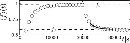
Figure 10: Average force $\langle f\rangle(t)$ as a function of time $t$. Symbols are results obtained from simulations. We set $k=10^{-7}\,\rm{N/m}$, $\omega_{r}=0.05\,\rm{s}^{-1}$ and $\omega_{\text{on}}=75\,\rm{s}^{-1}$. At $t=20000\,\rm{s}$, $\omega_{\text{on}}$ is diluted down to $\omega_{\text{on}}=50\,\rm{s}^{-1}$. Solid line represents a fit with an exponential decay (53) to the simulated data with fit parameter $\tau_{d}=1762\,\rm{s}$. Dashed lines indicate the average force in the initial state $f_{i}$ before dilution and in the new final state $f_{f}$ after dilution.

The relaxation dynamics to the new steady state after tubulin dilution is therefore governed by the average velocity $v(\langle f\rangle)$ given by eq. (45). To extract a characteristic relaxation time scale, we expand the average velocity $v(\langle f\rangle)$ to first order around the final steady-state polymerization force $f_{f}\equiv\langle f\rangle_{f}$, which is the solution of eq. (46) with $\omega_{r}$ and the decreased tubulin on-rate $\omega_{\text{on}}$, which takes its dilution value. Using $v(f_{f})=0$ one finds in first order

$$v(\langle f\rangle) \approx -\left[\frac{v_{+}(f_{f})\omega_{r}+v_{-}\omega_{c}^{\prime}(f_{f})}{\omega_{r}+\omega_{c}(f_{f})}\right]\left(\langle f\rangle-f_{f}\right)$$ (52)

where the prime denotes the derivative with respect to the force. In the last approximation we used the mean field condition eq. (46) and $v_{+}[f(x)]\approx v_{+}(0)e^{-f(x)}$, which is valid for $\omega_{\text{on}}\gg\omega_{\text{off}}$ (see eq. (13)). This expansion is only valid for average forces close to the new average polymerization force $f_{f}$. Using this expansion, the time evolution (51) of the average force after dilution exhibits an exponential decay

$$\langle f\rangle(t)=f_{f}+(f_{i}-f_{f})e^{-t/\tau_{d}}$$ (53)

with a characteristic dilution time scale

$$\tau_{d}=\frac{F_{0}}{k}\frac{\omega_{r}+\omega_{c}(f_{f})}{v_{+}(f_{f})\omega_{r}+v_{-}\omega_{c}^{\prime}(f_{f})}\approx\frac{F_{0}}{k}\frac{\omega_{r}+\omega_{c}(f_{f})}{2v_{-}\omega_{c}(f_{f})}$$ (54)

where we approximated the catastrophe rate by an exponential $\omega_{c}[f(x)]\approx\omega_{c}(0)e^{f(x)}$ according to eq. (15), and we used the mean field condition eq. (46). In the limit $\omega_{c}(f_{f})\gg\omega_{r}$, i.e., at forces $f_{f}\gg 1$, we obtain the simple result $\tau_{d}\approx F_{0}/2v_{-}k$. In general, the relaxation time $\tau_{d}$ is proportional to the square $\sigma^{2}$ of the width of the stationary distribution, cf. eq. (44): A narrow length distribution gives rise to fast relaxation to the new average force.

VII Experimental catastrophe model

So far we have employed the catastrophe rate derived by Flyvbjerg et al., to which we will refer as $\omega_{c,\text{Flyv}}$ in the following. This expression for the catastrophe rate was based on theoretical calculations of the inverse passage time to a state with a vanishing GTP-cap, see eq. (10). In order to investigate the robustness of our results with respect to changes of the catastrophe model, we now investigate an alternative expression for the catastrophe rate that has been obtained from experimental results. Throughout this section, we focus on the third confinement scenario of an elastic obstacle, and we compare results from the two different catastrophe models for zero rescue rate $\omega_{r}=0$ and non-zero rescue rate $\omega_{r}>0$. In addition, we restrict the comparison to mean field results, since numerical and stochastic calculations match mean field results well over the complete range of parameters (see Sec. VI).

Experimentally, it has been found that the average time $\langle\tau_{+}\rangle$ spent in a growing state is a linear function of the growth velocity $v_{+}$ Janson2003 . The force-dependent catastrophe rate is then given by

$$\omega_{c,\text{Jans}}(f)=\frac{1}{av_{+}(f)+b}$$ (55)

with constant coefficients $a=1.38\cdot 10^{10}\,{\rm s}^{2}{\rm m}^{-1}$ and $b=20\;{\rm s}$. At $v_{+}(f)=0$, $\omega_{c,\text{Jans}}(f)=0.05\,{\rm s}^{-1}$ and for $v_{+}(f)=-b/a$, the catastrophe rate $\omega_{c,\text{Jans}}(f)$ diverges. This is in contrast to the theoretical model, where $\omega_{c,\text{Flyv}}(f)$ is finite for all $v_{+}(f)$. Also $\omega_{c,\text{Jans}}(f)$ increases exponentially for forces $F>F_{0}$ or $f>1$. This common feature is essential and lead to similar results for both catastrophe models. In Fig. 11, both catastrophe rates are shown as a function of the dimensionless force $f$. The catastrophe model (55) is based on experimental data and, thus, is phenomenological. It assumes neither a purely chemical model, as in the model by Flyvbjerg et al., nor a chemo-mechanical model in the sense of “structural plasticity” Kueh2009 .

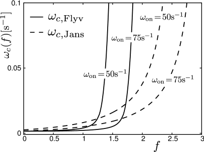
Figure 11: Catastrophe rate $\omega_{c}(f)$ as a function of force $f$ for $\omega_{\text{on}}=50\;\rm{s}^{-1}$ and $\omega_{\text{on}}=75\;\rm{s}^{-1}$. Solid lines: $\omega_{c,\text{Flyv}}$ from the catastrophe model by Flyvbjerg et al. Dashed lines: $\omega_{c,\text{Jans}}$ from the experimental catastrophe model by Janson et al.

VII.1 Vanishing rescue rate

We start with the case $\omega_{r}=0$ without rescue events, and we calculate the average maximal polymerization force within the experimental catastrophe model using the self-consistent mean field eq.  (32), which holds independently of the choice of catastrophe model (see Sec. VI.1). As for the catastrophe by Flyvbjerg et al., we have $\omega_{c,\text{Jans}}\tau\gg 1$ for realistic parameter values and $v_{+}(\langle f\rangle)<-b/a$, and eq. (32) can be solved explicitly for $\langle f_{\text{max}}\rangle$ in this limit. We find an average maximal polymerization force

$$\langle f_{\text{max}}\rangle\approx\ln\left(\left[\left(A^{2}+B\right)^{1/2}-A\right]\right)$$ (56)

with

$$A \equiv\frac{(\omega_{\text{on}}/\omega_{\text{off}}-1)ad\omega_{\text{off}}-(\omega_{\text{on}}/\omega_{\text{off}}-1)b-\tau}{2\tau}$$

$$B \equiv\frac{(\omega_{\text{on}}/\omega_{\text{off}}-1)ad\omega_{\text{on}}}{\tau}.$$

Since $\omega_{\text{on}}/\omega_{\text{off}}\gg 1$, eq. (56) can be approximated by

$$\langle f_{\text{max}}\rangle\approx\ln\left(\omega_{\text{on}}/\omega_{\text{max}}\right)$$ (57)

with

$$\omega_{\text{max}}\equiv\frac{2\tau\omega_{\text{off}}}{\left[\left(ad\omega_{\text{off}}-b\right)^{2}+4ad\omega_{\text{off}}\tau\right]^{1/2}-\left[ad\omega_{\text{off}}-b\right]}$$ (58)

For realistic parameter values, we have $\tau\gg ad\omega_{\text{off}}\geq b$, and recover the expression (34) derived using the Flyvbjerg catastrophe model:

$$\langle f_{\text{max}}\rangle\approx\frac{1}{2}\ln\left(\frac{\omega_{\text{on}}^{2}ad}{\omega_{\text{off}}\tau}\right)\approx\frac{1}{2}\ln\left(\frac{\omega_{\text{on}}dk}{F_{0}\omega_{c,\text{Jans}}(0)}\right).$$ (59)

In Fig. 12 (a), $\langle f_{\text{max}}\rangle$ as obtained from eq. (32) with the Flyvbjerg catastrophe model and eq. (56) with the experimental catastrophe model are shown as a function of $\omega_{\text{on}}$. Results match qualitatively and quantitatively well, although they are obtained from two different catastrophe models. The maximal polymerization force $\langle f_{\text{max}}\rangle$ always remains smaller than the stall force $f_{\text{stall}}$.

Figure 12: (a): Average maximal polymerization force $\langle f_{\text{max}}\rangle$ as a function of $\omega_{\text{on}}$ and $\omega_{r}=0$ for $k=10^{-7}\,{\rm N/m}$, $10^{-6}\,{\rm N/m}$ and $10^{-7}\,{\rm N/m}$ (top to bottom) . Dotted line: dimensionless stall force $f_{\text{stall}}$. Solid lines: $\langle f_{\text{max}}\rangle$ obtained from $\omega_{c,\text{Flyv}}$ (eq. (32)). Dashed lines: $\langle f_{\text{max}}\rangle$ obtained from $\omega_{c,\text{Jans}}$ (eq. (56)). (b): Average steady state force $\langle f\rangle$ as a function of $\omega_{\text{on}}$. $k=10^{-7}\,{\rm N/m}$, $\omega_{r}=0.2\,{\rm s}^{-1}$ (top) and $\omega_{r}=0.03\,{\rm s}^{-1}$(bottom). Solid lines: $\langle f\rangle$ obtained from $\omega_{c,\text{Flyv}}$ (eq. (46)). Dashed lines: $\langle f\rangle$ obtained from $\omega_{c,\text{Jans}}$ (eq. (60)). Dotted line: dimensionless stall force $f_{\text{stall}}$.

VII.2 Non-zero rescue rate

Now we compare both catastrophe models for a non-zero rescue rate, and we calculate the average steady state force. For the experimental catastrophe rate (55), the mean field equation (46) can be solved explicitly, and the average steady-state force $\langle f\rangle$ is given by

$$\langle f\rangle=\ln\left(\omega_{\text{on}}/\omega_{\text{av}}\right),$$ (60)

with

$$\omega_{\text{av}}\equiv\left(\left(\frac{b}{2ad}\right)^{2}+\frac{v_{-}}{\omega_{r}ad^{2}}\right)^{1/2}-\frac{b}{2ad}+\omega_{\text{off}}$$ (61)

Again $\langle f\rangle<f_{\text{stall}}$ since $\omega_{\text{av}}>\omega_{\text{off}}$. Fig. 12 (b) show $\langle f\rangle$ as a function of $\omega_{\text{on}}$. For realistic parameter values, we have $v_{-}/\omega_{r}\gg b^{2}/a$ and $(v_{-}/\omega_{r}ad^{2})^{1/2}\gg\omega_{\text{off}}$, and recover the expression (48) derived using the Flyvbjerg catastrophe model:

$$\langle f\rangle\approx\frac{1}{2}\ln\left(\frac{\omega_{\text{on}}^{2}\omega_{r}ad^{2}}{v_{-}}\right)\approx\frac{1}{2}\ln\left(\frac{v_{+}(0)\omega_{r}}{v_{-}\omega_{c,\text{Jans}}(0)}\right).$$ (62)

In Fig. 12 (b), results for $\langle f\rangle$ from both catastrophe models are shown as a function of on-rate $\omega_{\text{on}}$. The average steady state force obtained from $\omega_{c,\text{Flyv}}$ is always slightly larger than $\langle f\rangle$ obtained from $\omega_{c,\text{Jans}}$, since $\omega_{c,\text{Jans}}(f)>\omega_{c,\text{Flyv}}(f)$ for forces smaller than or comparable to $F_{0}$. Otherwise, both results agree qualitatively and quantitatively well.

VIII Force-velocity relation

Finally, we discuss the influence of the force-velocity relation on the MT dynamics. We restrict our analysis to mean field results obtained for the third scenario, i.e., the elastic obstacle. A change in the force-velocity relation directly modifies the velocity of growth $v_{+}(f)$, but it also affects the catastrophe rate $\omega_{c}(v_{+}(f))$, which are both crucial parts of the MT dynamics. In the following, we employ a more general form of the force-velocity relation, which is consistent with thermodynamic constraints, and we show that our results are robust with respect to this generalization.

In their investigation of experimental data Kolomeisky et al. used a generalized growth velocity

$$v_{+}(f,\theta)=d\{\omega_{\text{on}}\exp(-\theta f)-\omega_{\text{off}}\exp[(1-\theta)f]\},$$ (63)

which depends on a dimensionless “load distribution factor” $\theta$ Kolo2001 . The load distribution factor $\theta\in[0,1]$ determines whether the on- or off-rates are affected by external force, while keeping the ratio of overall on- and off-rate unaffected. Under force both the tubulin on-rate $\omega_{\text{on}}$ and the tubulin off-rate $\omega_{\text{off}}$ now acquire an additional Boltzmann-like factor. For $\theta=1$, we obtain again $v_{+}(f)$ as given by eq. (13). The dimensionless stall force is unaffected by $\theta$ and is still given by $f_{\text{stall}}=\ln\left(\omega_{\text{on}}/\omega_{\text{off}}\right)$.

VIII.1 Vanishing rescue rate

We use the generalized force-velocity relation $v_{+}(f,\theta)$ given by eq. (63) and the catastrophe rate $\omega_{c,\text{Flyv}}(f)$ in order to calculate the average maximal polymerization force $\langle f_{\text{max}}\rangle$ from the self-consistent mean field eq. (32). In Fig. 13 (a), $\langle f_{\text{max}}\rangle$ is shown as a function of the load distribution factor $\theta$ for $k=10^{-5}\,\rm{N/m}$ and different values of $\omega_{\text{on}}$. At $\theta=1$, the maximal force $\langle f_{\text{max}}\rangle$ equals the maximal polymerization force obtained with $v_{+}(f)$ from eq. (13). With decreasing $\theta$, $\langle f_{\text{max}}\rangle$ increases but remains below the dimensionless stall force. The growth velocity $v_{+}(f,\theta)$ increases with decreasing $\theta$ for a fixed force $f$ and, therefore, the maximal polymerization force $\langle f_{\text{max}}\rangle$ increases. For high tubulin on-rates $\omega_{\text{on}}=75-100\,\rm{s}^{-1}$ and small $\theta\approx 0,\ldots,0.2$, the maximal polymerization force $\langle f_{\text{max}}\rangle$ approaches the dimensionless stall force.

VIII.2 Non-zero rescue rate

For non-zero rescue rate, the average steady state force $\langle f\rangle$ is calculated from the mean field eq. (46), where we use the force-velocity relation $v_{+}(f,\theta)$ (eq. 63) and the catastrophe rate $\omega_{c,\text{Flyv}}(f)$. In Fig. 13 (b), results for $\langle f\rangle$ are shown as a function of $\theta$ for $k=10^{-7}\,\rm{N/m}$, $\omega_{r}=0.05\,\rm{s}^{-1}$ and different values of $\omega_{\text{on}}$. At $\theta=1$, $\langle f\rangle$ equals the average steady state force obtained with a velocity $v_{+}(f)$ taken from eq. (13). The average steady state force $\langle f\rangle$ increases with decreasing $\theta$, as explained above. For high tubulin on-rates $\omega_{\text{on}}=75-100\,\rm{s}^{-1}$ and small $\theta\approx 0,\ldots,0.2$ , also the average steady state force $\langle f\rangle$ again approaches the dimensionless stall force but remains smaller.

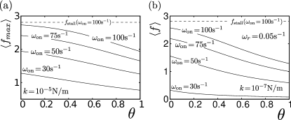
Figure 13: (a): Solid lines: Average maximal polymerization force $\langle f_{\text{max}}\rangle$ as a function of $\theta$ for $k=10^{-5}\,\rm{N/m}$ and different values of $\omega_{\text{on}}$. Dashed line: Dimensionless stall force $f_{\text{stall}}$ for $\omega_{\text{on}}=100\,\rm{s}^{-1}$. (b): Solid lines: Average steady state force $\langle f\rangle$ as a function of $\theta$ for $k=10^{-7}\,\rm{N/m}$, $\omega_{r}=0.05\,\rm{s}^{-1}$ and different values of $\omega_{\text{on}}$. Dashed line: Dimensionless stall force $f_{\text{stall}}$ for $\omega_{\text{on}}=100\,\rm{s}^{-1}$.

IX Discussion and conclusion

We studied MT dynamics in three different confining scenarios: (i) confinement by fixed rigid walls, (ii) an open system under constant force, and (iii) MT growth against an elastic obstacle with a force that depends linearly on MT length. These three scenarios represent generic confinement scenarios in living cells or geometries, which can be realized experimentally in vitro. For all three scenarios, we are able to quantify the MT length distributions. In scenario (iii) of an elastic obstacle, stochastic MT growth also gives rise to a stochastic force. For this model, we also quantify the average polymerization force generated by the MT in the presence of the dynamic instability.

The parameter $\lambda$, see (4) and (26), governs the MT length distributions in confinement by fixed rigid walls, and under a constant force. For confinement by rigid walls we introduced a realistic model for wall-induced catastrophes. There is a transition from exponentially increasing to exponentially decreasing length distributions if $\lambda$ changes sign. The average MT length is increasing for increasing on-rate and increasing rescue rate, as shown in Figs. 2. Wall-induced catastrophes lead to an overall increase in the average catastrophe frequency, which we quantify within the model.

For MT growth under a constant force, there exists a transition between bounded and unbounded growth as in the absence of force. This transition takes place where the parameter $\lambda(f)$ changes sign. Under force, the transition to unbounded growth is shifted to higher on-rates or higher rescue rates and determines a critical force $f_{c}$, see Figs. 4.

MT growth under a MT length-dependent linear elastic force allows for regulation of the generated polymerization force by experimentally accessible parameters such as the on-rate or the rescue rate. The force is no longer fixed but a stochastically fluctuating quantity because the MT length is a stochastic quantity. For zero rescue rate, i.e., in the absence of rescue events, we find that the average maximal polymerization force $\langle f_{\text{max}}\rangle$ before a catastrophe depends logarithmically on the tubulin concentration and is always smaller than the stall force in the absence of dynamic instability as shown in Fig. 5.

For a non-zero rescue rate, we find a steady state length distribution, which becomes increasingly sharply peaked for increasing rescue rate and is tightly controlled by microtubule growth parameters, see Figs. 6. Interestingly, the average microtubule length self-organizes such that the average steady state polymerization force $\langle f\rangle$ equals the critical force for the boundary of bounded and unbounded growth, $\langle f\rangle=f_{c}$. Because of the sharply peaked MT length distribution, the average polymerization force $\langle f\rangle$ can be calculated rather accurately within a mean field approach as can be seen in Figs. 7 and 8. The average polymerization force is always smaller than the stall force in the absence of dynamic instability.

Within this mean field approach, we can also describe the dynamics of the average force, see Figs. 9. This might be useful in modeling dilution experiments, where the response to sudden changes in the on-rate is probed. For this type of experiment, we estimate typical polymerization force relaxation times.

Finally, we show that our findings are robust against changes of the catastrophe model (Figs. 12) as long as the catastrophe rate increases exponentially above a characteristic force and that results are also robust against variations of the relation between force and polymerization velocity in the growing phase (Figs. 13), which are obtained by introducing a load distribution factor.

X Acknowledgments

We acknowledge financial support by the Deutsche Forschungsgemeinschaft (KI 662/4-1).

Appendix A Literature values for parameters

Ref.	$v_{+}(0)$ [m/s]	$\omega_{\text{on}}$ [1/s]	$v_{-}$ [m/s]	$\omega_{r}$ [1/s]
Drechsel Drechsel1992	$(0.7\;...\;2)\cdot 10^{-8}$	$(11\;...\;32)$	$\sim 1.8\cdot 10^{-7}$	-
Gildersleeve Gildersleeve1992	$\sim 4.2\cdot 10^{-8}$	$\sim 68$	$\sim 4.2\cdot 10^{-7}$	-
Walker Walker1988	$(4\;...\;8)\cdot 10^{-8}$	$(63\;...\;130)$	$\sim 5\cdot 10^{-7}$	$(0.05\;...\;0.08)$(TUB)
Laan Laan2008	$\sim 4.2\cdot 10^{-8}$	$68.25$	-	-
Janson Janson2004	$(3\;...\;4.3)\cdot 10^{-8}$	$(53\;...\;74)$	-	-
Pryer Pryer1992	-	-	-	$...\;0.5$ (TUB) $..\,0.15$ (MAPS)
Dhamodharan Dhamodharan1995	-	-	-	$...\;0.07$ (Cell) $\quad...\;0.085$ (MAPS)
Nakao Nakao2004	-	-	-	$...\;0.1$ (TUB)
Shelden Shelden1993	-	-	-	$(0.03\;...\;0.2)$ (Cell)

Table 1: Literature values for parameters. TUB: in vitro results for tubulin solutions, Cell: in vivo results, MAPS: effect from MT associated proteins. Values for $\omega_{\text{on}}$ are estimated from measured growth velocities via $\omega_{\text{on}}\approx v_{+}(0)N/d$ neglecting $\omega_{\text{off}}=6\,{\rm s}^{-1}$ Janson2004 . Here $N=13$ denotes the number of protofilaments within a single MT.

Parameter	$v_{-}\;[\rm{m/s}]$ (see Table 1)	$\omega_{\text{off}}\;[\rm{s}^{-1}]$	$d\;[\rm{m}]$	$r\;[\rm{m}^{-1}\rm{s}^{-1}]$	$v_{h}\;[\rm{m/s}]$	$\Delta t\;[\rm{s}]$
Value	$3\cdot 10^{-7}$	$6$	$0.6\cdot 10^{-9}$	$3.7\cdot 10^{6}$	$4.2\cdot 10^{-9}$	$0.1$

Table 2: Fixed parameter values for calculations and simulations.

References

- (1) R.D. Vale, Ann. Rev. Cell Biol. 3, 347 (1987).
- (2) J. Howard, Mechanics of Motor Proteins and the Cytoskeleton, Sinauer Associates,Inc., 2001.
- (3) M. Dogterom and B. Yurke, Science 278, 856 (1997).
- (4) M. Dogterom, J.W.J. Kerssemakers, G. Romet-Lemonne, M.E. Janson, Curr. Opin. Cell Biol. 17, 67 (2005).
- (5) R.R. Daga, A. Yonetani and F. Chang, Curr. Biol. 16, 1544 (2006).
- (6) S.E. Siegrist and C.Q. Doe, Genes & Dev. 21, 483 (2007).
- (7) R. Picone, X. Ren, K.D. Ivanovitch, J.D.W. Clarke, R.A. McKendry, and B. Baum, PLoS Biol. 8, e1000542 (2010).
- (8) L. Dehmelt, F.M. Smart, R.S. Ozer and S. Halpain, J. Neurosci. 23 , 9479 (2003).
- (9) T. Mitchison and M. Kirschner, Nature 312, 237 (1984).
- (10) C. Faivre-Moskalenko and M. Dogterom, Proc. Nat. Acad. Sci. USA 99, 16788 (2002).
- (11) H.T. Schek, M.K. Gardner, J. Cheng, D.J. Odde and A.J. Hunt, Curr. Biol. 4, 1053 (2007).
- (12) J.W.J. Kerssemakers, E.L. Munteanu, L. Laan, T.L. Noetzel, M.E. Janson and M. Dogterom, Nature 442, 7103 (2006).
- (13) L. Laan, J. Husson, E.L. Munteanu, J.W.J. Kerssemakers and M. Dogterom, Proc. Nat. Acad. Sci. USA 105, 8920 (2008).
- (14) C.M. Waterman-Storer, R.A. Worthylake, P.B. Liu, K. Burridge and E.D. Salmon, Nature Cell. Biol. 1, 45 (1999).
- (15) T. Mitchison and M. Kirschner, Neuron, 1, 761 (1988).
- (16) O.C. Rodriguez, A.W. Schaefer, C.A. Mandato, P. Forscher, W.M. Bement and C.M. Waterman-Storer, Nature Cell Biology 5, 599 (2003).
- (17) C.A. Athale, A. Dinarina, M. Mora-Coral, C. Pugieux, and F. Nedelec and E. Karsenti, Science 322, 1243 (2008).
- (18) E. Nogales, Ann. Rev. Biochem. 69, 277 (2000).
- (19) A. Akhmanova and M. Steinmetz, Nature Rev. Mol. Cell Biol. 9, 309 (2008).
- (20) F. Verde, M. Dogterom, E. Stelzer, E. Karsenti, S. Leibler, J. Cell Biology 118, 1097 (1992).
- (21) M. Dogterom and S. Leibler, Phys. Rev. Lett. 70, 1347 (1993).
- (22) B.M. Mulder, Phys. Rev. E 86, 011902 (2012).
- (23) M.E. Janson and M. Dogterom, Phys. Rev. Lett. 92, 248101 (2004).
- (24) H.Y. Kueh and T.J. Mitchison, Science 325, 960 (2009).
- (25) H. Flyvbjerg, T.E. Holy, and S. Leibler, Phys. Rev. Lett. 73, 2372 (1994).
- (26) H. Flyvbjerg, T.E. Holy and S. Leibler, Phys. Rev. E 54, 5538 (1996).
- (27) X. Li, J. Kierfeld and R. Lipowsky, Phys. Rev. Lett. 103, 048102 (2009).
- (28) X. Li, R. Lipowsky and J. Kierfeld, EPL 89, 38010 (2010).
- (29) M. Abramowitz and A.I. Stegun, Handbook of Mathematical Functions (National Bureau of Standards, Washington, 1965).
- (30) C.S. Peskin, G.M. Odell, and G.F. Oster, Biophys. J. 65, 316 (1993).
- (31) M.K. Gardner, M. Zanic, C. Gell, V. Bormuth, and J. Howard, Cell 147, 1092 (2011).
- (32) T.E. Holy and S. Leibler, Proc. Nat. Acad. Sci. USA 91, 5682 (1994).
- (33) M. Dogterom and B. Yurke, Phys. Rev. Lett. 81, 485 (1998).
- (34) B.S. Govindan and W.B. Spillman, Phys. Rev. E, 70, 032901 (2004).
- (35) Y.A. Komarova, I.A. Vorobjev and G.G. Borisy, J. Cell Sci. 115 3527 (2002).
- (36) C. Tischer, P.R. ten Wolde, and M. Dogterom, Biophys. J. 99, 726 (2010).
- (37) P. A. Curmi, S. S. L. Andersen, S. Lachkar, O. Gavet, E. Karsenti, M. Knossow, and A. Sobel, J. Biol. Chem. 272, 25029 (1997).
- (38) R. A. Walker, N. K. Pryer, and E. D. Salmon, J. Cell Biol. 114, 73 (1991).
- (39) M. Janson, M. de Dood, and M. Dogterom, J. Cell Biol. 161, 1029 (2003).
- (40) A. B. Kolomeisky and M. E. Fisher, Biophysical Journal 80, 149 (2001).
- (41) D.N. Drechsel, A.A. Hyman, M.H. Cobb, and M.W. Kirschner, Mol. Biol. Cell 3, 1141 (1992).
- (42) R.F. Gildersleeve, A.R. Cross, K.E. Cullen, A.P. Fagen, and R.C. Williams, J. Biol. Chem. 267, 7995 (1992).
- (43) R.A. Walker, E.T. O’Brien, N.K. Pryer, M.F. Soboeiro, W.A. Voter, H.P. Erickson, and E.D. Salmon, J. Cell Biol. 107, 1437 (1988).
- (44) N.K. Pryer, R.A. Walker, V.P. Skeen, B.D. Bourns, M.F. Soboeiro, and E.D. Salmon, J. Cell Sci. 103, 965 (1992).
- (45) R. Dhamodharan and P. Wadsworth, J. Cell Science 108, 1679 (1995).
- (46) C. Nakao, T.J. Itoh, H. Hotani, and N. Mori, J. Biol. Chem. 279, 23014 (2004).
- (47) E. Shelden and P. Wadsworth, J. Cell Biol. 120, 935 (1993).