A photometric study of the hot exoplanet WASP-19b^,

Abstract

Context. The sample of hot Jupiters that have been studied in great detail is still growing. In particular, when the planet transits its host star, it is possible to measure the planetary radius and the planet mass (with radial velocity data). For the study of planetary atmospheres, it is essential to obtain transit and occultation measurements at multiple wavelengths.

Aims. We aim to characterize the transiting hot Jupiter WASP-19b by deriving accurate and precise planetary parameters from a dedicated observing campaign of transits and occultations.

Methods. We have obtained a total of 14 transit lightcurves in the r’-Gunn, I-Cousins, z’-Gunn, and I+z’ filters and 10 occultation lightcurves in z’-Gunn using EulerCam on the Euler-Swiss telescope and TRAPPIST. We also obtained one lightcurve through the narrow-band NB1190 filter of HAWK-I on the VLT measuring an occultation at 1.19 $\muup$m. We performed a global MCMC analysis of all new data, together with some archive data in order to refine the planetary parameters and to measure the occultation depths in z’- band and at 1.19 $\muup$m.

Results. We measure a planetary radius of $R_{p}=1.376\pm 0.046$ ${R}_{J}$, a planetary mass of $M_{p}=1.165\pm 0.068$ ${M}_{J}$, and find a very low eccentricity of $e=0.0077_{-0.0032}^{+0.0068}$, compatible with a circular orbit. We have detected the z’-band occultation at $3\sigma$ significance and measure it to be $\delta F_{occ,z^{\prime}}=352\pm 116$ ppm, more than a factor of 2 smaller than previously published. The occultation at 1.19 $\muup$m is only marginally constrained at $\delta F_{occ,NB1190}=1711_{-726}^{+745}$ ppm.

Conclusions. We show that the detection of occultations in the visible range is within reach, even for 1m class telescopes if a considerable number of individual events are observed. Our results suggest an oxygen-dominated atmosphere of WASP-19b, making the planet an interesting test case for oxygen-rich planets without temperature inversion.

1 Introduction

At the time of writing, about 290 planets have been confirmed as transiting in front of their parent stars. Via the precise measurement of transit lightcurves, we are able to constrain the planetary radius, orbital inclination, and mass (usually with the help of radial velocity measurements), hence the planetary density.

Transiting planets open up a window onto the study of planetary atmospheres, their structure and composition. High-precision spectroscopic or spectro-photometric observations of planetary transits allow us to search for wavelength dependencies in the effective planetary radius, and from there conclude on the molecular species present in the planetary atmosphere. Also, from the transit lightcurve an independent measurement of the stellar mean density can be obtained (Seager & Mallén-Ornelas 2003), which is particularly useful since it can be used to refine the host stars’ parameters, namely its radius and mass. Having more accurate knowledge of the stellar parameters directly translates into more accurate physical values for the planetary mass and radius. This has led to several campaigns that collect transit lightcurves of published planets, as done by, e.g., Holman et al. (2006) and Southworth et al. (2009). Because the parameter measured from transit lightcurves is not the planetary radius itself but, in fact, the dimming of the star by the planetary disk, these measurements are affected by the brightness distribution along the stellar disk, i.e. stellar limb darkening as well as occulted and nonocculted spots. Occulted dark spots or bright faculae lead to short-term flux variations during the transit as the planet passes areas of the star having a different temperature and thus a different brightness. Nonocculted spots alter the stellar brightness outside of the planet’s path, leading to a slight increase in the observed transit depth. Depending on the spot distribution on the stellar surface, spots cause a rotational modulation of the stellar flux, with typical amplitudes of a few percent in the optical and timescales of several days. While the effect on the transit depth is weak (100 ppm for a typical brightness variation and transit depth of both 1 %), it is within the precision needed to detect of elements through transmission spectroscopy. Next to these physical effects, ground-based photometric lightcurves are known to suffer from correlated noise due to airmass, seeing, or other external variations (Pont et al. 2006). These effects can be mitigated by choosing optimal observation strategies (such as staying on the same pixels during the whole observation and defocusing in order to improve the sampling of the PSF) but can rarely be completely prevented. In this work, we collect a large number of transit lightcurves from 1m class telescopes and combine them to find not only a very precise but also an accurate measurement of the overall transit shape.

Observing the occultation of a transiting planet (Charbonneau et al. 2005, Deming et al. 2005) allows us to measure the brightness ratio of planet and star and thus measure the flux emitted or, at shorter wavelengths reflected, by the planet. At optical wavelengths, occultations have been measured almost exclusively from space (Alonso et al. 2009, Snellen et al. 2009, Borucki et al. 2009) using the CoRoT and Kepler satellites. There have been few ground based observations (Sing & López-Morales 2009, López-Morales et al. 2010, Smith et al. 2011), and so far none of the detections has been independently confirmed. Observations of occultations in the infrared have been plentiful, both from space (starting with Charbonneau et al. 2005, Deming et al. 2005) and from the ground, e.g., de Mooij & Snellen (2009), Gillon et al. (2009), and Croll et al. (2010). These observations provide information on the composition and the temperature profile of the planetary atmospheres. Some planets, such as HD209458, show a temperature inversion at high altitudes (Knutson et al. 2008), which is usually attributed to high abundances of TiO and VO (Hubeny et al. 2003, Fortney et al. 2008). These molecules are efficient absorbers of the stellar radiation heating up the high altitude atmosphere. However, it is not yet clear why some planets show inversions while others do not. As the number of planets with characterized atmospheres increases, the presence of inversions is turning out not to depend only on either the incident stellar flux (Fortney et al. 2008) or the host star activity level (Knutson et al. 2010). Spiegel et al. (2009) argue that TiO might be depleted in many hot Jupiters by condensation and subsequent gravitational settling. Recently, Madhusudhan et al. (2011) have suggested an additional connection between the C/O ratio and the presence of an inversion, because in atmospheres dominated by carbon, the main absorbers TiO and VO are not abundant enough to cause an inversion. It is essential to increase the sample of well-studied transiting hot Jupiters and to provide accurate values for the measured occultation depths.

WASP-19b has been identified as a hot Jupiter by Hebb et al. (2010), based on data taken by the WASP survey (Pollacco et al. 2006). The slightly bloated ($\rho=0.44$ $\rho_{J}$) planet with a mass near that of Jupiter ($M_{P}=1.17M_{J}$) is orbiting an $m_{V}=12.3$ G8V dwarf with a period of $0.79$ days. At this close separation, the planet is assumed to have been undergoing orbital decay moving it to its current orbital position at 1.21 times the Roche limit (Hebb et al. 2010, Hellier et al. 2011). The star is known to be active showing a rotational modulation with a period of 10.5 days in the discovery lightcurves (Hebb et al. 2010). Also, anomalies in transit lightcurves attributed to spot crossings have been reported by Tregloan-Reed et al. (2012). The projected stellar rotation axis of WASP-19 is aligned with the planet’s orbit (Hellier et al. 2011, Albrecht et al. 2012, Tregloan-Reed et al. 2012).

Occultations of WASP-19b have been measured in the past by Gibson et al. (2010) and Anderson et al. (2010) using HAWK-I in the K and H bands, respectively, as well as by Anderson et al. (2011) using the Spitzer Space Telescope at 3.6, 4.5, 5.8, and 8.0 $\muup$m. Recently, Burton et al. (2012) have published a z’-band lightcurve obtained with ULTRACAM during one occultation of WASP-19b, claiming its detection at $880\pm 119$ ppm. From the ensemble of measurements, Anderson et al. (2011) and Madhusudhan (2012) determine that WASP-19b does not possess a temperature inversion. Using the z’-band value of Burton et al. (2012), models favor a C-rich atmosphere. For the eccentricity of WASP-19b, Anderson et al. (2011) derive a 3-$\sigma$ upper limit of $e<0.027$.

In this paper we present results from an intense observing campaign of transits and occultations of WASP-19 obtained in both the optical and IR light. We describe all observations and their reduction in Section 2 and give details on the modeling in Section 3. In Sections 4 and 5 we present and discuss the results before concluding in Section 6.

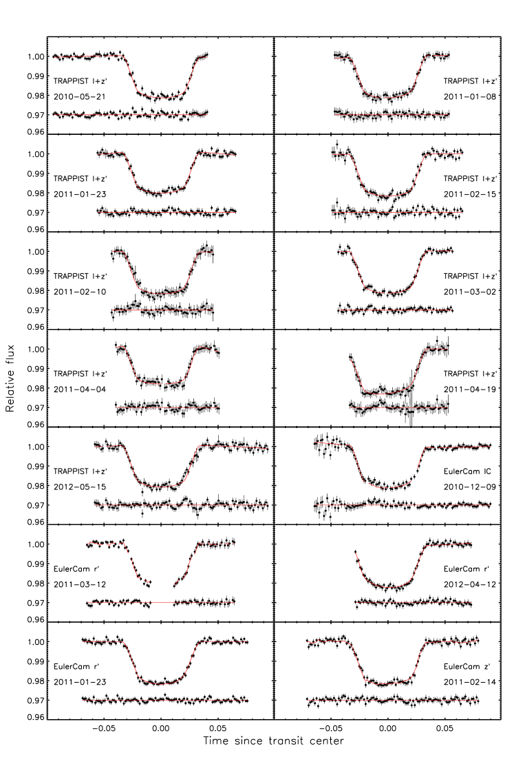
Figure 1: All transits observed together with their models and residuals. Instrument and filter used are indicated in each frame. All data have been binned in two-minute intervals.

2 Observations and data reduction

Between May 2010 and April 2012, we obtained a total of 25 lightcurves of WASP-19. Fourteen of these observations were timed to observe the transit, while 11 were performed during the occultation of the planet. We made use of three instruments: EulerCam at the 1.2 m Euler-Swiss Telescope and the automated 0.6 m TRAPPIST Telescope at ESO La Silla Observatory (Chile), as well as HAWK-I at the VLT/UT4 at ESO Paranal Observatory (Chile). We include in our analysis also the Faulkes South Telescope (FTS) lightcurve published by Hebb et al. (2010), the HAWK-I H-band observation by Anderson et al. (2010) and the radial velocity measurements presented in Hebb et al. (2010) and Hellier et al. (2011). All new observations are summarized in Table 1.

Date (UT)	Instrument	Filter	Eclipse Nature	Photometric Model Function	$\beta_{red}$	RMS [ppm, rel. flux, per 5 min]
2010-01-20	HAWK-I	NB1190	Occultation	$p(t^{2})$ and $p(t^{2})+p(FWHM^{1})$	1.23 and 1.11	$1820$ and $1096$
2010-05-21	TRAPPIST	I+z’	Transit	$p(t^{2})$	1.17	$680$
2010-12-09	EulerCam	IC	Transit	$p(t^{2})+p(sky^{1})$	1.30	$900$
2011-01-08	TRAPPIST	I+z’	Transit	$p(t^{2})$	1.62	$610$
2011-01-21	TRAPPIST	z’	Occultation	$p(t^{2})$	1.00	$720$
2011-01-23	EulerCam	r’	Transit	$p(t^{2})$	1.22	$570$
2011-01-23	TRAPPIST	I+z’	Transit	$p(t^{2})$	1.42	$730$
2011-02-10	TRAPPIST	I+z’	Transit	$p(t^{2})$	2.05	$1170$
2011-02-14	EulerCam	z’	Transit	$p(t^{2})+p(sky^{1})$	1.25	$700$
2011-02-15	TRAPPIST	I+z’	Transit	$p(t^{2})$	1.00	$840$
2011-02-23	TRAPPIST	z’	Occultation	$p(t^{2})$	1.51	$960$
2011-02-24	TRAPPIST	z’	Occultation	$p(t^{2})$	1.00	$690$
2011-03-02	TRAPPIST	I+z’	Transit	$p(t^{2})$	1.00	$610$
2011-03-12	EulerCam	r’	Transit	$p(t^{2})+p(FWHM^{2})$	1.38	$690$
2011-04-04	TRAPPIST	I+z’	Transit	$p(t^{2})$	1.82	$980$
2011-04-19	TRAPPIST	I+z’	Transit	$p(t^{2})$	1.80	$1120$
2011-04-21	TRAPPIST	z’	Occultation	$p(t^{2})$	1.00	$700$
2011-04-28	EulerCam	z’	Occultation	$p(t^{2})+p(FWHM^{1})$	1.19	$520$
2011-05-06	EulerCam	z’	Occultation	$p(t^{2})$	1.13	$400$
2012-02-28	EulerCam	z’	Occultation	$p(t^{2})$	1.00	$510$
2012-03-11	EulerCam	z’	Occultation	$p(t^{2})$	1.13	$440$
2012-03-15	EulerCam	z’	Occultation	$p(t^{2})+p(xy^{1})$	1.29	$800$
2012-03-18	EulerCam	z’	Occultation	$p(t^{2})+p(FWHM^{1})$	1.00	$460$
2012-04-12	EulerCam	r’	Transit	$p(t^{2})$	1.55	$940$
2012-05-15	TRAPPIST	I+z’	Transit	$p(t^{2})$	1.24	$970$

Table 1: A summary of newly obtained photometry. Date, instrument, filter, and the nature of eclipse are given for each observation together with the photometric model function, red noise amplitude $\beta_{red}$ (as defined in Winn et al. 2008) and the RMS of the binned (5 minutes) residuals. The notation $p(j^{i})$ refers to a polynomial of degree i of parameter j, e.g. $p(t^{2})$ denotes a polynomial of second degree with respect to time.

2.1 EulerCam

Five transit and six occultation lightcurves have been obtained with EulerCam, the imager of the Euler-Swiss telescope at La Silla. The instrument and the reduction of EulerCam data are described in detail by Lendl et al. (2012). The observations were done either with a focused telescope or applying a small $\leq$ 0.1 mm defocus yielding stellar PSFs with a typical full width at half-maximum (FWHM) between 1.1 and 2.5 arcsec, while the exposure times were between 60s and 120s, depending on filter and conditions. On 12 March 2011, the CCD temperature during the observations was slightly elevated, $-100^{\circ}$ C instead of the nominal $-115^{\circ}$ C. The lightcurves were extracted using relative aperture photometry, with the reference stars and apertures selected independently for each observation.

2.2 TRAPPIST

Nine transits and four occultations of WASP-19b were observed with the robotic 60 cm TRAPPIST (Gillon et al. 2011, Jehin et al. 2011) that is also located at the La Silla site. We defocused the telescope slightly in order to spread the light over more pixels yielding typical FWHM values between 3.6 and 6.5 arcsec on the images and used exposure times between 15s and 40s. Again, the lightcurves were obtained with relative aperture photometry, where IRAF is used in the reduction process.

2.3 HAWK-I

We obtained photometry of WASP-19 using the HAWK-I instrument (Pirard et al. 2004, Casali et al. 2006) on VLT UT4 during two occultations of WASP-19b using the narrow band filters NB1190 and NB2090. Unfortunately, during the NB2090 observations, the target exceeded the linearity range of the detector, as a consequence the data do not have the necessary precision to detect the occultation; however, the NB1190 data are good, and thus we restrict our analysis to them.

The NB1190 observations of WASP-19 took place on 20 January 2010 from 02:55 to 06:55 UT covering the predicted occultation time together with 145 min of observations outside of eclipse. The detector integration time (DIT) was kept short (3s) so the counts of the target and a bright reference star did not exceed the linear range of the detector. The data were obtained by alternating between two jitter positions, in order to be able to correct for background variations if necessary.

The data were corrected for dark and flat field effects using standard procedures. Then, we identified bad pixels on the images and substituted their values by the mean of the neighboring pixels. Here, we experimented with different cutoffs for the identification of bad pixels and obtained the best results discarding pixels deviating by 4 $\sigma$ for background values and 40 $\sigma$ for stars. The target flux was extracted from the corrected images using aperture photometry. We tested a set of constant apertures, as well as apertures that varied from image to image as a function of the stellar FWHM. The sky annulus was kept constant for all images. The best result was obtained using a variable aperture of two times the FWHM. We tested all bright stars of the four HAWK-I chips and found the best photometry using only the single bright star located on the same chip as WASP-19. The bright stars on the other detectors showed significantly different variations so were not used. The lightcurves are shown in Figure 2.

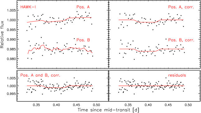
Figure 2: The occultation observed with HAWK-I at 1.19 $\muup$m on 20 January 2010. The lightcurves obtained from the two jitter positions are shown. Top panel: the raw lightcurves, together with the occultation and photometric model (left), and divided by the photometric model (right). Bottom panel: both lightcurves corrected and normalized with the best fit (left) and the residuals (right).

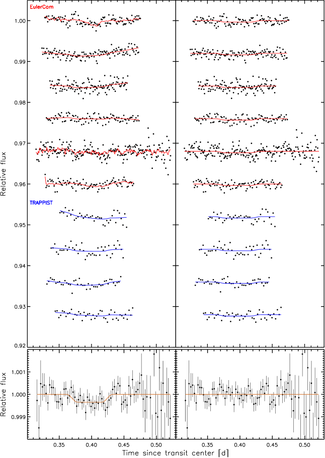
Figure 3: All occultation lightcurves obtained in the z’-band. The upper six lightcurves were obtained with EulerCam and are unbinned, while the lower four lightcurves were obtained with TRAPPIST and binned in two-minute intervals. Left panel: the raw lightcurves, together with the occultation and photometric models. Right panel: the lightcurves and the occultation model, divided by the photometric model. The lower panel shows all data, corrected for the photometric model and binned in four-minute intervals. Data and model are shown on the left, while the residuals are shown on the right.

3 Modeling

We performed a combined analysis of all photometric (transit and occultation) data, together with published radial velocities. The data were modeled using the Markov chain Monte Carlo (MCMC) method in order to derive the posterior probability distributions of the parameters of interest (see 3.1 for details). Incorporated in our analysis are models for photometric correction functions, which account for photometric variations not related to the eclipse, i.e. airmass, weather, or instrumental effects. We also rescale our error bars if they show to be underestimated. Please see Section 3.2 for details.

3.1 MCMC

We employed the MCMC method using the implementation described in Gillon et al. (2010, 2012). In short, the radial velocities are modeled using a Keplerian orbit and with the prescription of the Rossiter-McLaughlin effect (Rossiter 1924, McLaughlin 1924) provided by Giménez (2006). The photometric model for eclipses (transits and occultations) is that of Mandel & Agol (2002), used without limb darkening for occultations. The jump parameters are transit depth $dF$, impact parameter $b$, transit duration $d$, time of midtransit $T_{0}$, period $P$, occultation depths $dF_{occ}$ for each wavelength, and $K_{2}=K\sqrt{1-e^{2}}P^{1/3}$ (where $K$ and $e$ denote the radial velocity semi-amplitude and eccentricity, respectively). The jump parameters $\sqrt{e}\cos\omega$ and $\sqrt{e}\sin\omega$ (where $\omega$ denotes the argument of periastron) are used to determine of the eccentricity. Limb darkening is accounted for by using the combinations $c_{1}=2u_{1}+u_{2}$ and $c_{2}=u_{1}-2u_{2}$ of the calculated limb-darkening coefficients of Claret & Bloemen (2011) following Holman et al. (2006). With the exception of the limb darkening parameters (for which we use a normal prior with a width equal to the error quoted by Claret & Bloemen 2011), we assume uniform prior distributions. We followed the method described by Enoch et al. (2010) using the mean stellar density, temperature, and metallicity for determining the stellar mass and radius. In our whole analysis, we always ran at least two MCMC chains and checked convergence with the Gelman & Rubin test (Gelman & Rubin 1992). All time stamps are converted to the TDB time standard, as described by Eastman et al. (2010).

3.2 Photometric model and error adaptation

As described in Section 1, ground-based lightcurves are often affected by red noise correlated with external parameters. In our MCMC analysis, we have the possibility to include time, FWHM, coordinate shifts, and background variations in our model. This is done by multiplying the transit model by a polynomial (up to 4th degree) with respect to any combination of these parameters. The coefficients of the polynomial are not included as jump parameters in the MCMC but are found by minimization of the residuals at each step. In order to account for airmass and stellar variability effects, we assumed a second-order polynomial with respect to time as the minimal accurate model for ground-based photometry. We checked more complex models by running MCMC chains of $10^{5}$ points on each lightcurve including higher orders of time dependence and additional terms in FWHM, pixel position and background. A more complex model was favored over a simple one only if the Bayes factor (Schwarz 1978) estimated from the Bayesian information criterion indicated a significantly higher probability (i.e. $B_{1,2}>100$). The best photometric model functions are listed in Table 1 and were used in all subsequent analyses. For the H-band data, we kept the coordinate dependence described in Anderson et al. (2010), and the archive FTS lightcurve (Hebb et al. 2010) was fitted with the minimal model.

Although photometric error bars are usually derived including scintillation, readout, background, and photon noise, they are often underestimated, and we adapted them by accounting for additional white and red noise. For the white noise, we derived a scaling factor $\beta_{w}$ from the ratio of the mean photometric error and the standard derivation of the photometric residuals. For the red noise, we obtained a scaling factor $\beta_{r}$ by comparing the standard deviation of the binned photometric residuals to the standard deviation of the complete dataset, as described in detail by Winn et al. (2008) and Gillon et al. (2010). Finally we multiplied both scaling factors to obtain the correction factors $CF=\beta_{w}\times\beta_{r}$ for the photometric errors. In the subsequent analysis, all photometric error bars were multiplied by these factors. Analogously, we computed values for the radial velocity jitter that were added quadratically to the radial velocity errors.

3.3 Summary of tested models

Having derived the above factors, we analyzed the entire dataset. We did so by running chains of $10^{5}$ points on all photometric and radial velocity data. Next to the global analysis, we also performed analyses of subsets of lightcurves (described in detail in Sections 4.1 and 4.3.3). Additionally, we searched for any color dependence in the transit depths by allowing for depth offsets between the different filters (Section 4.3.2) and also derived individual midtransit times in order to check for transit-timing variations (Section 4.3.2). To verify the result of Burton et al. (2012), we performed a global analysis in which we included their value, $DF_{occ,z^{\prime}}=880\pm 190$ ppm, as a Gaussian prior (Section 4.3.3). The results are described in detail in Section 4, while all newly obtained lightcurves are shown in Figure 1 (transits), Figure 2 (NB1190 occultation), and Figure 3 (z’-band occultations).

4 Results

4.1 The TRAPPIST transit sequence

To investigate the benefits of combining several lightcurves, we divided our set of nine I+z’ TRAPPIST transit lightcurves into subsets containing all possible combinations of one to nine lightcurves and performed an MCMC analysis on each of them using the procedure described in Section 3. We can observe how the solutions converge as we use an increasing number of transits in Figure 4. The outlier located at high transit depth stems from the transit observed on 10 February 2011, which is showing very high red noise. It is clearly visible that combinations favoring a large transit depth also require a larger transit width. This correlation might be related to the presence of star spots occulted by the planet. While spots on the limb of the star shorten the apparent transit duration, spots closer to the center of the star will produce a flux increase leading to a decrease in the apparent transit depth. It is also possible that the overall stellar variability is not well constrained, e.g. due to little or no out-of-transit data, and thus the photometric correction model cannot be determined correctly. Figure 4 also shows the global solution and the solution obtained from the EulerCam transits alone. The results from TRAPPIST and EulerCam agree within their error bars, yet the EulerCam data find a slightly larger transit depth, width, and impact parameter.

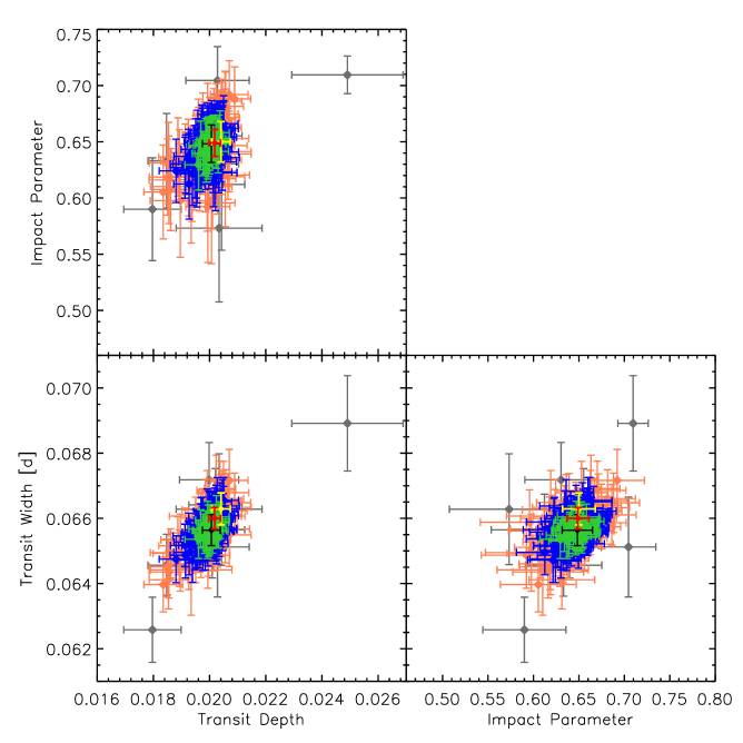
Figure 4: The solutions found from fits to all possible subsets of TRAPPIST transits are shown. The single transits are shown in gray, and combinations of three, five and seven transits are shown in orange, blue and green, respectively. The solution to all TRAPPIST and EulerCam lightcurves are shown in black and yellow, respectively. The global solution is shown in red.

Next to investigating the parameters obtained from combinations of transits, one can also check the photometric improvement reached by combining an increasing number of lightcurves. To measure this effect, we used each set of combinations of $n=1$ to $n=9$ lightcurves, folded them on the best-fit period, and binned the data. Points before -0.05 and after +0.05 days from transit center were discarded to avoid phases that are not covered by all lightcurves. In Figure 5, we show the photometric RMS against the number of combined lightcurves and compare the decrease in RMS to the “best case” (decrease with $\frac{1}{\sqrt{n}}$). The increase in precision is near that value, particularly if small time bins are used. By combining all nine TRAPPIST lightcurves, we obtain an RMS of 321 ppm for a moderately sized time bin of five minutes.

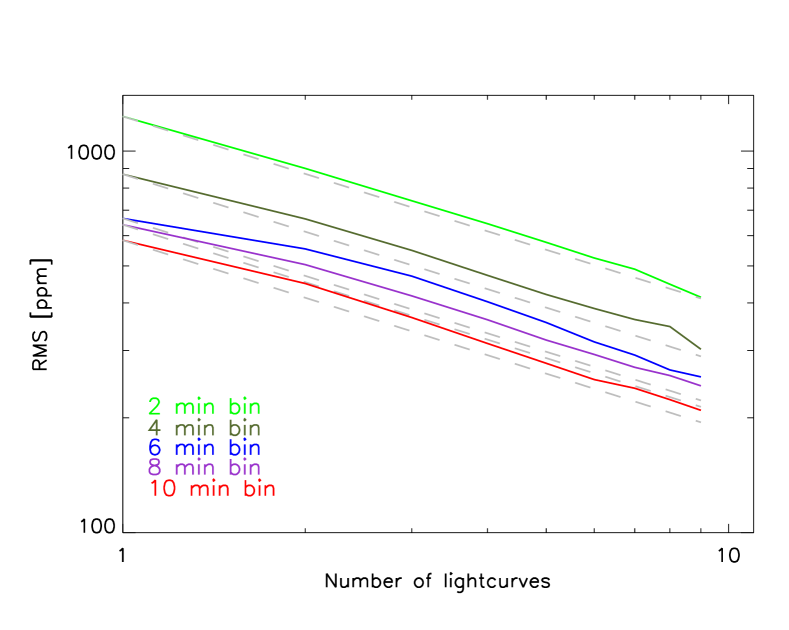
Figure 5: The increase in photometric precision by combining up to nine lightcurves from TRAPPIST. The RMS in bin sizes of (from top to bottom) two, four, six, eight and ten minutes are shown. The gray dashed lines show the expected $1/\sqrt{n_{lc}}$ decrease for each time bin.

4.2 One simultaneous observation

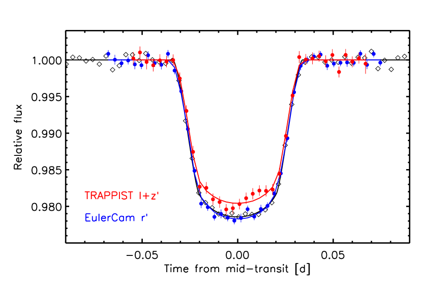
Figure 6: The simultaneous transit observation performed with TRAPPIST (red) and EulerCam (blue). For clarity, the data are binned into 5-minute bins, and the models of the individual transits are shown as solid lines. The binned data from the combination of all I+z’ lightcurves (same as in Figure 8) are shown in black for comparison.

The transit of 23 January 2011 was observed with EulerCam and TRAPPIST simultaneously, using an r’-Gunn filter on EulerCam and an I+z’ filter on TRAPPIST. Figure 6 depicts the two lightcurves superimposed. It is obvious that the TRAPPIST data are showing an anomalously small transit depth and a short-term brightening during the second half of the transit. With only one lightcurve, one might conclude that the planet crossed a star spot during transit. Since the EulerCam light curve was observed at shorter wavelengths and given the cooler temperature of the spot, we would expect the effect to be more pronounced here. However, the feature is absent in the r’-band, excluding the spot-hypothesis. We tried to account for it by adopting photometric correction models including backgound, sky, and FWHM parameters, yet were not able to find a model that reproduced the lightcurve shape. Removing the points during the second half of the transit in the TRAPPIST lightcurve, we obtain a value within 1 $\sigma$ of the EulerCam result.

4.3 Global Analysis

We performed a global MCMC analysis using all available radial velocity and photometric data including transits and occultations (described in detail in Section 3). The results are shown in Table 2.

WASP-19
Jump parameters
Transit depth	$\Delta F=(R_{p}/R_{\ast})^{2}$	$0.02018\pm 0.00021$
	$b^{\prime}=a*\cos(i_{p})$ $[R_{\ast}]$	$0.649\pm 0.012$
Transit duration	$T_{14}$ [d]	$0.06586_{-0.00031}^{+0.00033}$
Time of midtransit	$T_{[0]}-2450000$ [HJD]	$6029.59204\pm 0.00013$
Period	$P$ [d]	$0.7888390\pm 2\times 10^{-7}$
	$K_{2}=K\sqrt{1-e^{2}}P^{1/3}$ [${\rm m\,s}^{-1}\,d^{1/3}$]	$238.1\pm 2.7$
z’-band occultation depth	$\Delta F_{occz^{\prime}}$ [ppm]	$352\pm 116$
NB1190 occultation depth	$\Delta F_{occNB1190}$ [ppm]	$1711_{-726}^{+745}$
H-band occultation depth	$\Delta F_{occH}$ [ppm]	$3216_{-455}^{+473}$
	$\sqrt{e}$ cos $\omega$	$0.053\pm 0.020$
	$\sqrt{e}$ sin $\omega$	$0.054_{-0.082}^{+0.057}$
	$\sqrt{v_{\ast}\sin{I_{\ast}}}$ cos $\beta$	$1.85_{-0.19}^{+0.17}$
	$\sqrt{v_{\ast}\sin{I_{\ast}}}$ sin $\beta$	$-0.27\pm 0.23$
	$c_{1,\rm r^{\prime}}=2u_{1,r}+u_{2,r}$	$1.123\pm 0.040$
	$c_{2,\rm r^{\prime}}=u_{1,r}-2u_{2,r}$	$-0.052\pm 0.037$
	$c_{1,\rm IC}=2u_{1,IC}+u_{2,IC}$	$0.903\pm 0.034$
	$c_{2,\rm IC}=u_{1,IC}-2u_{2,IC}$	$-0.173\pm 0.025$
	$c_{1,\rm I+z^{\prime}}=2u_{1,I+z^{\prime}}+u_{2,I+z^{\prime}}$	$0.840\pm 0.050$
	$c_{2,\rm I+z^{\prime}}=u_{1,I+z^{\prime}}-2u_{2,I+z^{\prime}}$	$-0.251\pm 0.053$
	$c_{1,\rm z^{\prime}}=2u_{1,z^{\prime}}+u_{2,z^{\prime}}$	$0.831\pm 0.029$
	$c_{2,\rm z^{\prime}}=u_{1,z^{\prime}}-2u_{2,z^{\prime}}$	$-0.218\pm 0.021$
Deduced parameters
Radial velocity semi-amplitude	$K$ [${\rm m\,s}^{-1}$]	$257.7\pm 2.9$
Planet radius	$R_{p}$ [${R}_{J}$]	$1.376\pm 0.046$
Planet mass	$M_{p}$ [${M}_{J}$]	$1.165\pm 0.068$
Planet density	$\rho_{p}$ [$\rho_{J}$]	$0.447_{-0.025}^{+0.027}$
Eccentricity	$e$	$0.0077_{-0.0032}^{+0.0068}$
Argument of periastron	$\omega$ [deg]	$43_{-67}^{+28}$
Semi-major axis	$a$ [AU]	$0.01653\pm 0.00046$
Normalized semi-major axis	$a/R_{\ast}$	$3.573\pm 0.046$
Inclination	$i_{p}$ [deg]	$79.54\pm 0.33$
Transit impact parameter	$b_{tr}$	$0.645\pm 0.012$
Occultation impact parameter	$b_{occ}$	$0.652\pm 0.015$
Time of midoccultation	$T_{occ}-2450000$ [HJD]	$6030.77766\pm 0.00088$
Projected spin-orbit angle	$\beta$ [deg]	$-8.4_{-7.2}^{+7.0}$
Planet equilibrium temperature	$T_{eq}$ [K]	$2058\pm 40$
Planet surface gravity	$\log g_{p}$ [cgs]	$3.184\pm 0.015$
Stellar mass	$M_{\ast}$ [${M}_{\sun}$]	$0.968_{-0.079}^{+0.084}$
Stellar radius	$R_{\ast}$ [${R}_{\sun}$]	$0.994\pm 0.031$
Stellar mean density	$\rho_{\ast}$ [$\rho_{\sun}$]	$0.983_{-0.036}^{+0.039}$
1st quadratic LD coeff., r’ band	$u_{1,\rm r^{\prime}}$	$0.439\pm 0.020$
2nd quadratic LD coeff., r’ band	$u_{2,\rm r^{\prime}}$	$0.246\pm 0.015$
1st quadratic LD coeff, I+z’ band	$u_{1,\rm I+z}$	$0.286\pm 0.026$
2nd quadratic LD coeff., I+z’ band	$u_{2,\rm I+z}$	$0.268\pm 0.019$
1st quadratic LD coeff., IC band	$u_{1,\rm IC}$	$0.326\pm 0.016$
2nd quadratic LD coeff., IC band	$u_{2,\rm IC}$	$0.2497\pm 0.0094$
1st quadratic LD coeff., z’ band	$u_{1,\rm z^{\prime}}$	$0.289\pm 0.014$
2nd quadratic LD coeff., z’ band	$u_{2,\rm z^{\prime}}$	$0.2536\pm 0.0077$

Table 2: The median values and the 1-$\sigma$ errors of the marginalized posterior PDF obtained from the MCMC analysis of all new data plus the radial velocities and lightcurves published by Hebb et al. (2010), Anderson et al. (2010) and Hellier et al. (2011).

4.3.1 Eccentricity

While Hebb et al. (2010) and Hellier et al. (2011) did not measure a significant nonzero eccentricity from the analysis of radial velocity and transit data, Anderson et al. (2010) presented for WASP-19b a value of $e=0.016^{+0.015}_{-0.007}$ from the timing of their H-band occultation. When including their data in our analysis, we derived a lower value for the eccentricity with a similar significance $0.0077_{-0.0032}^{+0.0068}$. Removing the H-band data, we obtained $0.0061_{-0.0043}^{+0.0063}$, clearly not significant. We therefore do not see any evidence for a nonzero eccentricity of the WASP-19 system.

4.3.2 Transit depth and timing variations

Filter	Wavelength (width) [nm]	$R_{p}/R_{\ast}$
r’-Gunn	664 (99)	$0.1437\pm 0.0013$
IC	760 (91)	$0.1336\pm 0.0026$
I+z’	838 (190)	$0.14171\pm 0.00094$
z’-Gunn	912.4 (68)	$0.1428\pm 0.0014$

Table 3: The planet/star radius ratios obtained from a global MCMC analysis, while allowing for filter-dependent transit depths. For the I+z’ and z’ filters, the widths given here have been determined from the combination of the filter transmission and detector response curves. For the r’ and IC filters we give the equivalent widths.

Epoch	Mid-transit time	O-C [min]	deviation in $\sigma$
	[$HJD_{TDB}-2450000$]
$-1537$	$4817.14633\pm 0.00021$	$-0.24\pm 0.30$	$0.8$
$-876$	$5338.56927\pm 0.00023$	$0.27\pm 0.33$	$0.8$
$-621$	$5539.72327\pm 0.00030$	$0.36\pm 0.44$	$0.8$
$-583$	$5569.69826\pm 0.00036$	$-0.92\pm 0.53$	$1.8$
$-564$	$5584.68693\pm 0.00024$	$0.12\pm 0.34$	$0.4$
$-564$	$5584.68684\pm 0.00019$	$-0.00\pm 0.28$	$0.0$
$-541$	$5602.83138\pm 0.00046$	$1.78\pm 0.67$	$2.7$
$-536$	$5606.77464\pm 0.00022$	$0.44\pm 0.32$	$1.4$
$-535$	$5607.56241\pm 0.00033$	$-1.10\pm 0.47$	$2.3$
$-516$	$5622.55057\pm 0.00026$	$-0.79\pm 0.38$	$2.1$
$-503$	$5632.80612\pm 0.00025$	$0.14\pm 0.36$	$0.4$
$-474$	$5655.68222\pm 0.00045$	$-0.19\pm 0.66$	$0.3$
$-455$	$5670.66976\pm 0.00064$	$-0.78\pm 0.93$	$0.8$
$0$	$6029.59250\pm 0.00035$	$0.67\pm 0.51$	$1.3$
$43$	$6063.51174\pm 0.00030$	$-0.54\pm 0.44$	$1.2$

Table 4: The midtransit times and their deviation from a linear ephemeris. The values were obtained from the combined analysis of all transits while the ephemeris was fixed to the one quoted in Table 2.

One of the checks we performed on the data was letting the transit depth vary for different filters, in order to search for any wavelength dependencies in the star/planet radii ratio which can be used to constrain models of the atmospheric transmission. The phase-folded and binned lightcurves for each filter are shown in Figure 8, and the respective radii ratios are shown in Figure 9 and listed in Table 3. The r’, I+z’, and z’ band values match very well, only the IC value is slightly lower, 2.6 $\sigma$ below the global solution.

We also searched for any deviation from a linear ephemeris by performing a global analysis while fixing the ephemeris to the ephemeris derived from the global analysis but letting the individual midtransit times vary. The results are shown in Figure 7 and listed in Table 4. While there is some (expected) scatter around the linear ephemeris, none of the deviations exceed 2.7 $\sigma$, so we find no evidence of TTVs in the WASP-19 system.

Figure 7: The O-C deviations of the individual transits from the ephemeris given in Table 2 are shown. The filled circle represents the FTS transit of Hebb et al. (2010), the squares represent data obtained with EulerCam, and the diamonds represent data from TRAPPIST.

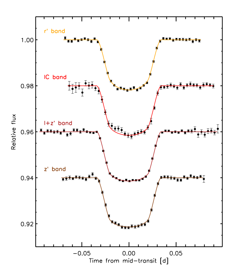
Figure 8: The combined lightcurves in each of the observed bands binned in five-minute intervals. The lightcurves are a combination of (from top to bottom) three, one, nine, and two observations. Using the displayed five-minute intervals, the RMS of the residuals in the interval [-0.05,0.05] days are (from top to bottom) 432, 1021, 321, and 487 ppm.

Figure 9: The planet/star radius ratios obtained from an MCMC analysis of all data, while allowing for filter-dependent transit depths. The errorbars in wavelength span the filters effective width. The deviation IC lightcurve is based on only a single observation.

4.3.3 z’- band and 1.19 $\muup$m occultations

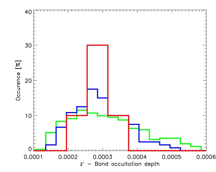
Figure 10: A histogram of the results obtained from modeling combinations of five (green), seven (blue), and nine (red) occultations.

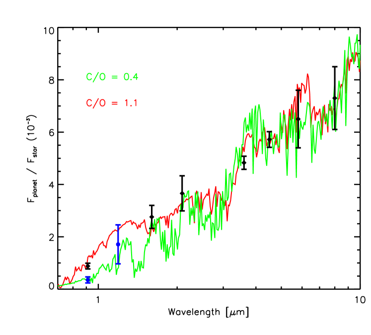
Figure 11: The model spectra of the dayside atmosphere of WASP-19b computed by Madhusudhan (2012) compared to observations. The z’-band and 1.19 $\muup$m observations presented in this work are shown in blue, while the data of Anderson et al. (2010, 2011), Burton et al. (2012) and Gibson et al. (2010) are shown in black. The two model atmospheres shown have been computed for the carbon-dominated (C/O = 1.1, red) and oxygen-dominated (C/O = 0.4, green) case and are reproduced here with kind permission of N. Madhusudhan.

We measure a z’- band occultation depth of $352\pm 116$ ppm from the combined analysis of the ten z’- band occultation lightcurves in our dataset. For individual lightcurves the occultation is well buried in the noise. To verify that our nonzero occultation depth is not caused by a systematic effect present in a single or a small number of lightcurves, we proceeded in a similar way to what we did with the set of TRAPPIST transits (Section 4.1). We created all possible subsets containing at least five occultation lightcurves and analyzed them while fixing all parameters except the occultation depth to the values derived above. Histograms of the derived occultation depths are shown in Figure 10. The results obtained from fits of fewer light curves are consistent with the presented value, although they have lower significance. Recently, Burton et al. (2012) have presented an occultation depth for WASP-19b of $880\pm 190$ ppm based on one lightcurve obtained with ULTRACAM mounted at the NTT telescope at ESO La Silla observatory. We tried to reproduce this value by using it as a Gaussian prior (with a width equal the error bar on the measurement) in our MCMC. Even with this prior, the resulting occultation depth is $466\pm{97}$ ppm. We are thus not confirming the measurement of Burton et al. (2012) but conclude that the occultation of WASP-19b in z’ band is significantly smaller.

In our global analysis we include the occultation observed with HAWK-I using the narrow-band NB1190 filter. From our data we measure the occultation depth at 1.19 $\muup$m to be $1711_{-730}^{+750}$ ppm.

5 Discussion

From the homogeneous set of TRAPPIST I+z’ lightcurves, we can evaluate the photometric improvement obtained from combining lightcurves. As presented in Figure 5, we are not far from the ideal case of only white noise. Even if combining as many as nine lightcurves, we are still gaining in photometric precision by adding additional transits.

Following our observation strategy of deriving the most accurate measurement of the overall transit shape and thus the planetary parameters, we can reduce correlated noise, which can drastically affect single lightcurves. This is most evident if the same transit is observed simultaneously using different instruments. In the case of a combination of nine TRAPPIST lightcurves, we measured the planet/star radius ratio with a precision of 0.7% in I+z’-band, while three observations with EulerCam in r’-band and a combination of two EulerCam lightcurves and an FTS yield slightly larger errors, giving a precision of 0.9 and 1.0 %. While these values agree well within their error bars, a single lightcurve obtained in IC-band gives a 2.6 $\sigma$ lower value. This lightcurve shows a small flux increase during transit (possibly the signature of a star spot), and we suggest that this possible radius variation be verified with additional data. Discarding this point, we see a flat optical transmission spectrum of WASP-19b. Overall, the values derived from our analysis are in good agreement with the values previously derived.

With two new occultation measurements, we can proceed to constrain the chemical composition and structure of the planetary atmosphere. For this purpose, we use the model spectra calculated by Madhusudhan (2012). In their work, they show models of WASP-19b for a carbon-dominated C/O = 1.1 and an oxygen-dominated C/O = 0.4 atmosphere. For oxygen-rich models, a strong absorption around 0.9 $\muup$m is expected from the TiO and VO leading to a smaller z’- band occultation depth. Following the occultation measurement by Burton et al. (2012), Madhusudhan (2012) tentatively classified WASP-19b as having a carbon-dominated atmosphere.

Comparing our values to these models (see Figure 11), we find our measurement of the z’- band matches the oxygen-rich model extremely well, showing higher absorption, indicative of higher abundances in TiO and VO. These elements require a higher concentration of oxygen in the planetary atmosphere in order to contribute measurably to the planetary spectrum. The 1.19 $\muup$m value matches the oxygen- and carbon-rich models equally well. Thus, we suggest WASP-19b is a highly irradiated oxygen-dominated planet, fitting the O2 or upper O1 Class defined by Madhusudhan (2012). This should be confirmed by a joint analysis of the previously published data and the measurements added in this work since the models of planetary emission are not unique.

From the Spitzer data on WASP-19b (Anderson et al. 2011), we know that WASP-19b does not show any temperature inversion. At first glance, this might seem unexpected for an oxygen-dominated atmosphere, because it is precisely the molecules of which we measure higher concentrations that are presumed to be causing temperature inversions. Still, as different wavelengths probe different depths in the planetary atmosphere, the z’- band observations probe a deeper atmospheric layer, which is below the expected temperature inversion. In this context it would be interesting to evaluate the effects of gravitational settling and stellar UV radiation on the presence and distribution of TiO and VO in the planetary atmosphere. TiO and VO might be destroyed or depleted from the upper atmosphere, thus inhibiting a temperature inversion, while lower in the atmosphere the intact TiO and VO could be causing the measured absorption in the z’ band.

6 Conclusion

We have carried out an in-depth observing campaign on WASP-19 collecting a total of 14 transit and 10 occultation lightcurves with EulerCam and TRAPPIST, as well as one 1.19 $\muup$m lightcurve with HAWK-I. From the large homogeneous set of nine TRAPPIST lightcurves, we demonstrate how both the attainable photometric precision and the accuracy of the derived parameters can be greatly improved by combining an increasing number of lightcurves.

We have detected the z’-band occultation of WASP-19b using 1m class telescopes by the combined analysis of our lightcurves. We measure it at $352\pm 116$ ppm, more than a factor of two smaller than previously published. From our HAWK-I data we obtain an occultation depth of $1711_{-730}^{+750}$ ppm at 1.19 $\muup$m. These results shed new light on the chemical composition of the planetary atmosphere, indicating a $C/O$ ratio of $C/O<1$, i.e. an oxygen-dominated atmosphere.