Statistical linearizations for stochastically quantized fields

Abstract

The statistical linearization method known in nonlinear mechanics and random vibrations theory has been applied to stochastically quantized fields in finite temperature. It has been shown that even in its simplest form the method yields convenient implicit equations for the self-energy, equivalent to the Dyson-Schwinger equations resulting from the summation of infinite number of perturbative diagrams. Three examples have been provided: the quantum anharmonic oscillator, the scalar $\phi^{4}$ theory in three spatial dimension, and the Bose-Hubbard model. The Ramanujan summation has been used to deal with divergent integrals and series.

I Introduction

The method of stochastic quantization invented in the end of seventies PW has immediately grasped interest of several members of the field-theoretical community, please see DH ; Namiki ; MS for reviews. The method has offered a version of the quantum theory in which one has to deal with $c$-number fields (instead of operators or path integrals) at the expense of introduction of another temporal dimension and Langevin forces. A very considerable amount of work has been applied to develop the theory and run simulations. In fact, it is the possibility of efficient simulations that has strongly stimulated the research in this method. Initially, it has been worked out as a way to obtain Euclidean vacuum expectation values of the (products of) quantum fields. Later, it has been demonstrated that the method can also work in the Minkowski space-time HR ; Gozzi . What is more, it has been shown that the stochastic quantization can also be used to obtain transition amplitudes between quantum states in simple quantum mechanical systems HN ; YN .

In spite of the initially vigorous development, the interest in stochastic quantization diminished considerably in the nineties. The present authors believe that this happened because of the following reasons: (i) the method has been worked out with the hope to offer efficient simulations of Yang-Mills fields, especially in quantum chromodynamics (QCD). However, the computational QCD has had in its disposal very efficient unrelated methods, and stochastic quantization has not seemed to offer much more advantage from the computational point of view; (ii) there have been serious difficulties in the simulations in Minkowski (rather than Euclidean) space due to the instabilities caused by the Langevin forces; (iii) it appears that the non-perturbative analytic or semi-analytic methods have been somewhat underdeveloped in the stochastic-quantization context - the only works on the subject of which are aware are the variational approaches of AD and BGG ; BG1 and Hartree-like technique of BG2 (the above four papers are virtually forgotten); (iv) the method has not been sufficiently tested on simpler quantum systems - for instance, one would expect that before difficult lattice QCD simulations are launched, the stochastic quantization should first demonstrate that it allows to get, say, correct values of the ground-state energy of the helium atom.

The objective of the paper is to address the point (iii) and demonstrate that the stochastic quantization can very easily import well-known non-perturbative techniques from the non-linear mechanics as well as the physics of random vibrations. Here, we use the simplest of those methods, namely, that of statistical linearization Booton ; Kazakov ; Caughey ; AU ; Ito , please see also RS ; Socha for reviews. It allows one to replace a non-linear term in a Langevin equation with such a linear term that the expectation value of the resulting error is minimized. However, there exist also several other linearization criteria. We mention here the minimization of the energy error, equality of mean-square energies, and equality of mean-square system functions (i.e. the deterministic parts of the right-hand sides of corresponding Langevin equations).

Our analyses provided below may be classified as a specfic version of Hartree-like approach. The equations of motion in the additional time-like variables are linearized and the linear parameters which enter them are found variationally on assuming a Gaussian distribution of fields. Since the Hartree approaches have been discussed in multitude of papers, there is a natural question whether it is profitable to investigate it again. The present authors believe that it is indeed the case because the simplest version of statistical linearization presented here is only a necessary first step towards developing more sophisticated and non-trivial approximation schemes based on the so-called higher-order linearization as well as building statistically equivalent non-linear solvable models. Less importantly, we have not found any discussion of a Hartree-like approximation in the context of stochastic quantization except of BG2 where it has been introduced, so to say, “by hand” rather than with the help of a systematic procedure like the one described below.

The main part of the paper is organized as follows. To introduce the technique of statistical linearization in the stochastic-quantization context, the quantum anharmonic oscillator in non-zero temperature is considered in Section 2. Temperature-dependent corrections to its frequency are obtained. In Section 3, we consider the Langevin equations for $\phi^{4}$ theory in three spatial dimensions and finite temperature. We show that the statistical linearization technique provides us with the correct self-consistent equation for the self-energy. Its zeroth-temperature limit is analyzed using the Ramanujan summation of divergent series. Section 4 contains an analysis of the Bose-Hubbard model from the point of view of stochastic quantization. The Langevin equations are again linearized and Dyson-Schwinger-like equation for the self-energy is obtained. Section 5 contains some concluding remarks.

II Anharmonic oscillator

Let us consider the anharmonic oscillator described by the following Euclidean action (confer NK ):

$$S_{E}=\int_{0}^{\beta{\hbar}}\left[\frac{1}{2}m{\dot{x}}^{2}+\frac{1}{2}m\omega^{2}x^{2}+\frac{m\lambda}{4!}x^{4}\right]d\tau,$$ (1)

Ito where $\tau$ is the Euclidean time, $x$ is the position of the oscillator, $m$ - its mass, $\omega$ denotes the frequency of the free oscillations, $\beta$ is inverse temperature, and ${\lambda}$ parametrizes the strength of nonlinearity.

According to the prescription of the stochastic quantization, $x$ should satisfy the equation:

$$\frac{dx}{ds}=-\frac{\delta S_{E}}{\delta x}+\eta(s,\tau),$$

where $\delta/\delta x$ denotes the functional derivative, and $s$ is an additional independent variable of the temporal character while $\eta(s,\tau)$ is a Gaussian Langevin “force” which satisfies the following conditions:

$$\langle\eta(s,t)\rangle=0,\;\;\;\;\;\langle\eta(s,\tau)\eta(s^{\prime},\tau^{\prime})\rangle=2{\hbar}\delta(s-s^{\prime})\delta(t-t^{\prime}).$$ (2)

Explicitly, the pseudo-dynamics in “time” $s$ is governed by the following non-linear stochastic diffusion equation:

$$\frac{dx}{ds}=m\frac{d^{2}x}{d\tau^{2}}-m\omega^{2}x-m\frac{\lambda}{3!}x^{3}+\eta(s,\tau).$$ (3)

It has been proved PW ; DH that the Euclidean, ground-state correlation functions $\langle x(t_{1})x(t_{2})...x(t_{n})\rangle$ can be obtained by taking the limit:

$$lim_{s\rightarrow\infty}\langle x(t_{1})x(t_{2})...x(t_{n})\rangle_{\eta},$$

where the subscript $\eta$ denotes the averaging over the stochastic forces $\eta$. Taking the limit is equivalent to the averaging by using a stationary solution to the Fokker-Planck equation corresponding to the Langevin equation (3).

We look for the stationary ($s\rightarrow\infty$) solution of Eq.(3) subject to periodic boundary condition in the Euclidean time $\tau$ to include finite temperature:

$$x(s,0)=x(s,\beta{\hbar}).$$

By “stationary” solution” of (3) we mean the inhomogeneous part of the general solution corresponding to $s$ sufficiently large that the initial values of $x(s)$ give vanishing contribution as they are exponentially damped.

Due to the boundary conditions, it is reasonable to expand:

$$x(s,\tau)=\sum_{\nu=-\infty}^{\infty}x_{\nu}(s)u_{\nu}(\tau),$$

where

$$u_{\nu}(\tau)=\frac{1}{\sqrt{\beta{\hbar}}}\exp(2\pi i\nu\tau/\beta{\hbar})=\frac{1}{\sqrt{\beta{\hbar}}}\exp(i\omega_{\nu}\tau).$$

The stochastic force can be expanded in the same way:

$$\eta(s,\tau)=\sum_{\nu=-\infty}^{\infty}\eta_{\nu}(s)u_{\nu}(\tau),$$

with $\langle\eta_{\nu}(s)\eta_{\rho}(s^{\prime})\rangle=(2{\hbar})\delta_{\nu,-\rho}\delta(s-s^{\prime})$.

The amplitudes $x_{\nu}(s)$ satisfy:

$$\frac{dx_{\nu}}{ds}=-m(\omega_{\nu}^{2}+\omega^{2})x_{\nu}-m\frac{{\lambda}}{3!\beta{\hbar}}\sum_{\rho,\sigma}x_{\rho}x_{\sigma}x_{\nu-\rho-\sigma}+\eta_{\nu}(s).$$ (4)

Now, we are in position to look for an equivalent linear system. It has to take the form:

$$\frac{dx_{\nu}}{ds}+m\Omega_{\nu}^{2}x_{\nu}=\eta_{\nu}(s).$$ (5)

The statistical linearization technique in its simplest version consists of subtracting the equations (4 - 5), taking the square of the resulting error, summing over all $\nu$ and taking the expectation value. This expectation value should be computed with respect to the distribution function of $x_{\nu}$ obtained by solving the full nonlinear system. As it is, however, not available, we approximate that expectation value by its value obtained from the linearized system (5). Thus, we need to minimize the expression:

$$E=m\sum_{\nu}\langle|(\omega_{\nu}^{2}+\omega^{2})x_{\nu}+\frac{{\lambda}}{3!\beta{\hbar}}\sum_{\rho,\sigma}x_{\rho}x_{\sigma}x_{\nu-\rho-\sigma}-\Omega_{\nu}^{2}x_{\nu}|^{2}\rangle$$ (6)

The absolute value in the above expression appears naturally because $x_{\nu}$ are, naturally, complex; they must satisfy, however, the condition $x_{-\nu}=x_{\nu}^{\star}$ because $x$ itself is real. Differentiating with respect to $\Omega_{\nu}$ and equating to zero the obtained derivative $\partial E/\partial\Omega_{\mu}^{2}$ gives the following implicit equation for $\Omega_{\mu}^{2}$:

$$\Omega_{\mu}^{2}=\omega_{\mu}^{2}+\omega^{2}+\frac{{\lambda}}{3!\beta{\hbar}}\frac{\sum_{\rho,\sigma}\langle x_{-\mu}x_{\rho}x_{\sigma}x_{\mu-\rho-\sigma}\rangle}{\langle x_{\mu}x_{-\mu}\rangle}$$ (7)

For Gaussian distribution of $x_{\mu}$, the above ratio of moments can be simplified RS :

$$\Omega_{\mu}^{2}=\omega_{\mu}^{2}+\omega^{2}+\frac{{\lambda}}{3!\beta{\hbar}}\langle\frac{\partial}{\partial x_{\mu}}\sum_{\rho,\sigma}x_{\rho}x_{\sigma}x_{\mu-\rho-\sigma}\rangle,$$ (8)

so that $\Omega_{\mu}^{2}$ depends only on the second moments of $x_{\mu}$:

$$\Omega_{\mu}^{2}=\omega_{\mu}^{2}+\omega^{2}+\frac{\lambda}{2\beta{\hbar}}\sum_{\nu}\langle x_{\nu}x_{-\nu}\rangle.$$ (9)

Now, the system (5) can be solved immediately to give for $s\rightarrow\infty$:

$$\langle x_{\nu}x_{-\nu}\rangle=\frac{\hbar}{m\Omega_{\nu}^{2}}$$

Let us now write $\Omega_{\nu}^{2}=\omega_{\nu}^{2}+\omega^{2}+\Pi$. Then the “self-energy” $\Pi$ satisfies the self-consistent equation:

$$\Pi=\frac{\lambda}{2m\beta}\sum_{\nu}\frac{1}{\omega_{\nu}^{2}+\omega^{2}+\Pi}$$ (10)

Performing now the frequency summation we find that $\Pi$ must satisfy:

$$\Pi=\frac{{\hbar}\lambda}{2m\sqrt{\omega^{2}+\Pi}}\left(1+2n_{B}(\sqrt{\omega^{2}+\Pi})\right),$$ (11)

where $n_{B}(x)$ is the Bose-Einstein factor $(\exp(\beta{\hbar}x)-1)^{-1}$.

In Fig. 1 there is a shaded contour plot of the dependence of the $\Pi/\omega^{2}$ on dimensionless coupling constant $L={\hbar}\lambda/(2m\omega^{3})$ and dimensionless inverse temperature $b=\beta{\hbar}\omega$.

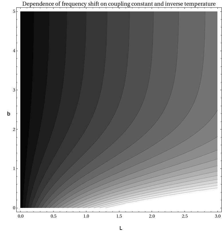
Figure 1: Dependence of the $\Pi/\omega^{2}$ on dimensionless coupling constant $L={\hbar}\lambda/(2m\omega^{3})$ and dimensionless inverse temperature $b=\beta{\hbar}\omega$. The lighter regions correspond to larger values of the $\Pi/\omega^{2}$

.

Let us observe that the dependence of $\Pi$ on $\lambda$ is non-analytic even for zeroth temperature. Thus, the result is, in a sense, ”non-perturbative”.

III Statistical linearization of non-linear scalar field theory

We start with the following Euclidean action for the $\phi^{4}$ model:

$$S_{E}=\int_{0}^{\beta{\hbar}}d\tau\int d^{3}x{\mathcal{L}}_{E},$$ (12)

where

$${\mathcal{L}}_{E}=\frac{1}{2c^{2}}(\partial_{\tau}\phi)^{2}+\frac{1}{2}(\nabla\phi)^{2}+\frac{1}{2{\hbar}^{2}}m^{2}c^{2}\phi^{2}+\frac{g}{4!}\phi^{4}.$$ (13)

The resulting Langevin equation for $\phi$ reads

$$\frac{\partial\phi}{\partial s}=\frac{1}{c^{2}}\frac{\partial^{2}\phi}{\partial\tau^{2}}+\nabla^{2}\phi-\frac{m^{2}c^{2}}{{\hbar}^{2}}\phi-\frac{g}{3!}\phi^{3}+\eta(s,t,{\bf r}).$$ (14)

We impose periodic boundary conditions in the Euclidean time, $\phi(s,0,{\bf r})=\phi(s,\beta{\hbar},{\bf r})$. Also, as it is convenient to work with discrete variables, we initially assume that $\phi$ is also periodic in each spatial variable, that is, $\phi$ is defined in the box of the volume $L_{0}^{3}$ with periodic boundary condition imposed in each spatial direction. At the end of calculations we shall take the limit $L_{0}\rightarrow\infty$. Thus, we expand:

$$\phi(s,\tau,{\bf r})=\frac{1}{\sqrt{\beta{\hbar}V}}\sum_{\lambda}\sum_{{\bf k}}\exp(-i\omega_{\lambda}\tau)\exp(i{\bf k}{\bf r})\phi_{\lambda{\bf k}},$$ (15)

where $\omega_{\lambda}=2\pi\lambda/\beta{\hbar}$, ${\bf k}=(2\pi/L_{0})(m,n,p)$, and $\lambda$, $m$, $n$, $p$ are integers.

Upon a similar Fourier decomposition of the stochastic forces we obtain:

$$\frac{d\phi_{\lambda{\bf k}}}{ds}=-\left(\frac{\omega_{\lambda}^{2}}{c^{2}}+{\bf k}^{2}+\frac{m^{2}c^{2}}{{\hbar}^{2}}\right)\phi_{\lambda{\bf k}}-\frac{g}{3!\beta{\hbar}L_{0}^{3}}N_{\lambda{\bf k}}+\eta_{\lambda{\bf k}},$$ (16)

where

$$N_{\lambda{\bf k}}=\sum_{\lambda_{1},\lambda_{2}}\sum_{{\bf k}_{1},{\bf k}_{2}}\phi_{\lambda_{1},{\bf k}_{1}}\phi_{\lambda_{2},{\bf k}_{2}}\phi_{\lambda-\lambda_{1}-\lambda_{2},{\bf k}-{\bf k}_{1}-\bf k_{2}}.$$ (17)

The corresponding linear system takes the form:

$$\frac{d\phi_{\lambda{\bf k}}}{ds}=-A_{\lambda{\bf k}}\phi_{\lambda{\bf k}}+\eta_{\lambda{\bf k}}.$$ (18)

Using the same prescription as before, i.e., minimization of the expectation value of the error, we find:

$$A_{\lambda{\bf k}}=\frac{\omega_{\lambda}^{2}}{c^{2}}+{\bf k}^{2}+\frac{m^{2}c^{2}}{{\hbar}^{2}}+\frac{1}{2}\frac{g}{\beta{\hbar}L_{0}^{3}}\sum_{\lambda_{1}{\bf k}_{1}}\langle\phi_{\lambda_{1}{\bf k}_{1}}\phi_{-\lambda_{1},-{\bf k}_{1}}\rangle$$ (19)

On writing

$$A_{\lambda{\bf k}}=\frac{\omega_{\lambda}^{2}}{c^{2}}+{\bf k}^{2}+\frac{m^{2}c^{2}}{{\hbar}^{2}}+\Pi$$

and taking expectation values with respect to the Gaussian probability density associated with the linear system, we obtain:

$$\Pi=\frac{g}{2\beta L_{0}^{3}}\sum_{\mu}\sum_{{\bf k}}\frac{1}{\omega_{\mu}^{2}/c^{2}+{\bf k}^{2}+m^{2}c^{2}/{\hbar}^{2}+\Pi},$$ (20)

or by taking the limit $L_{0}\rightarrow\infty$,

$$\Pi=\frac{g}{2(2\pi)^{3}\beta}\sum_{\mu}\int d^{3}k\frac{1}{\omega_{\mu}^{2}/c^{2}+{\bf k}^{2}+m^{2}c^{2}/{\hbar}^{2}+\Pi}.$$ (21)

This is a self-consistent, temperature-dependent equation for the self-energy of the self-interacting non-linear scalar field. It agrees with that derived in Altherr (please see also LeBellac ). Needless to say, the really serious analysis starts precisely at this point. It must involve both the mass and coupling constant renormalization, and has been performed, e.g., in DHLR ; BIR . It has been found that the separation of the zero-temperature and temperature-dependent terms as well as determination of the thermal mass is surprisingly non-trivial, KR . In view of the fact that the matter has been carefully discussed in the above papers, we shall not give any detailed analysis of our own. We would only like to investigate briefly the consequences of application to Eq. (21) of the so-called Ramanujan technique of summation of divergent series. But before doing this we would like to observe that, while there is nothing new in Eq. (21), we have obtained it practically effortlessly using the simplest, and actually trivial, version of statistical linearization of stochastically quantized theory. No diagrammatic analyses or functional differentiation or integration have been necessary.

Let us perform the frequency summation as well as the angular integration in Eq. (21). The expression for $\Pi$ takes now the form:

$$\Pi = \frac{g{\hbar}c}{8\pi^{2}}\int_{0}^{\infty}\frac{k^{2}dk}{\sqrt{k^{2}+m^{2}c^{2}/{\hbar}^{2}+\Pi}}\cdot$$ (22)

$$\cdot\left(1+2n_{B}(c\beta{\hbar}\sqrt{k^{2}+m^{2}c^{2}/{\hbar}^{2}+\Pi})\right).$$

The integral of the first term on the right-hand side is obviously quadratically divergent.

Let us have a closer look at the limit $\beta\rightarrow\infty$. The second term (which contains a convergent integral) on the right-hand side vanishes in that limit. The self-consistent expression for the self-energy takes then the form:

$$\Pi = \frac{g{\hbar}c}{8\pi^{2}}\int_{0}^{\infty}\frac{k^{2}dk}{\sqrt{k^{2}+(m^{2}c^{2}/{\hbar}^{2})+\Pi}}=$$ (23)

$$=\frac{g{\hbar}cp^{2}}{8\pi^{2}}\int_{0}^{\infty}\frac{\kappa^{2}d\kappa}{\sqrt{\kappa^{2}+1}},$$

where $p^{2}=(m^{2}c^{2}/{\hbar}^{2})+\Pi$ and we assume that $p^{2}>0$. Euler’s substitution $\sqrt{\kappa^{2}+1}=-\kappa+u$ yields:

$$\Pi = \frac{g{\hbar}cp^{2}}{32\pi^{2}}\int_{1}^{\infty}\frac{(u^{2}-1)^{2}}{u^{3}}=$$ (24)

$$=\frac{g{\hbar}cp^{2}}{32\pi^{2}}\left(\int_{1}^{\infty}udu-2\int_{1}^{\infty}\frac{du}{u}+\frac{1}{2}\right).$$

In order to deal with the above divergent integrals let us invoke the Abel-Plana formula CE :

$$\int_{0}^{\infty}f(x)dx=\sum_{n=0}^{\infty}f(n)-\frac{1}{2}f(0)-i\int_{0}^{\infty}\frac{f(it)-f(-it)}{e^{2\pi t}-1}dt.$$ (25)

It makes sense if both the integrals and the series converge. However, let us make use of the following definition. We say that an integral $\int_{0}^{\infty}f(x)dx$ is summable in the Ramanujan sense if the sum of the series $\sum_{n=0}^{\infty}f(n)$ in the Ramanujan sense Delabaere ; Moreta exists, and the integral

$$\int_{0}^{\infty}(f(it)-f(-it))/(e^{2\pi t}-1)dt$$

converges in the ordinary sense. Then we write:

$${}^{(R)}\int_{0}^{\infty}f(x)dx=^{(R)}\sum_{n=0}^{\infty}f(n)-\frac{1}{2}f(0)-i\int_{0}^{\infty}\frac{f(it)-f(-it)}{e^{2\pi t}-1}dt.$$ (26)

with obvious meaning of the superscript $(R)$.

What is called here the “Ramanujan summation” of divergent series consists in the following. Let $\sum_{n\geq 1}a(n)$ be a formal (divergent) series, and let $R(x)=\sum_{n\geq 0}a(n+x)$. Then, if $R(x)$ satisfies the difference equation $R(x)-R(x+1)=a(x)$, the value $R(1)$ gives the sum of the series $\sum_{n\geq 1}a(n)$. The sum is unique if we additionally require fulfillment of the condition $\int_{1}^{2}R(x)=0$ and $a(n)$ does not grow too fast with $n$. In Delabaere an algorithm to compute $R(x)$ in terms of the Borel transform of $a(n)$ as a well as a useful table of the Ramanujan sums of some divergent series is given.

With the above definitions in mind, we can investigate the question of summability of divergent integrals in Eq. (24) in the Ramanujan sense.

We find immediately:

$${}^{(R)}\int_{1}^{\infty}udu = {}^{(R)}\int_{0}^{\infty}udu-\frac{1}{2}=-\frac{1}{2}+^{(R)}\sum_{n=0}^{\infty}n+$$ (27)

$$+2\int_{0}^{\infty}\frac{t}{e^{2\pi t}-1}dt.$$

As the last integral is equal to $1/12$, we have:

$${}^{(R)}\int_{1}^{\infty}udu=-\frac{5}{12}+^{(R)}\sum_{n=0}^{\infty}n.$$ (28)

But, according to Delabaere ,

$${}^{(R)}\sum_{n=1}^{\infty}n^{k}=\frac{1-B_{k+1}}{k+1},$$

where $B_{k}$ are the Bernoulli numbers. Hence ${}^{(R)}\sum_{n=1}^{\infty}n=5/12$, and

$${}^{(R)}\int_{1}^{\infty}udu=0.$$

What is more,

$${}^{(R)}\int_{1}^{\infty}\frac{du}{u}=^{(R)}\sum_{n=0}^{\infty}\frac{1}{n+1}-\frac{1}{2}-2\int_{0}^{\infty}\frac{t}{(t^{2}+1)(e^{2\pi t}-1})dt.$$ (29)

Using now the fact that in the Ramanujan sense the sum of the harmonic series is the Euler-Mascheroni constant $\gamma$ while

$$-2\int_{0}^{\infty}\frac{t}{(t^{2}+z^{2})(e^{2\pi t}-1)}dt=\psi(z)+\frac{1}{2z}-log(z),$$

where $\psi(z)$ is the digamma function Lebedev (please see the formula 6.3.21 of AS ), we find that, quite trivially,

$${}^{(R)}\int_{1}^{\infty}\frac{du}{u}=0,$$ (30)

because $\psi(1)=-\gamma$.

As a result of the Ramanujan summation, we get in the zeroth-temperature limit:

$$\Pi=\frac{g{\hbar}c}{64\pi^{2}}\left(\frac{m^{2}c^{2}}{{\hbar}^{2}}+\Pi\right),$$ (31)

or

$$\Pi=\frac{g_{ren}{\hbar}c}{64\pi^{2}}\frac{m^{2}c^{2}}{{\hbar}^{2}}$$ (32)

with $g_{ren}=g/(1-(g{\hbar}c/64\pi^{2}))$.

Thus the “renormalization” of the coupling constant appears to be finite (provided that $g{\hbar c}\neq 64\pi^{2}$), and the same is true about the correction to the mass. This is possible only because we have performed a summation of two divergent integrals. In the present case, the Ramanujan approach resulted in their trivial elimination.

We would like to repeat that the formal manipulation with divergent series in the spirit of Ramanujan cannot be thought of as a substitution of the detailed and careful renormalization procedure. Nonetheless, the former is perhaps of non-vanishing interest and may be worth of some further study.

IV Bose-Hubbard model

Let us now consider the one-dimensional Bose-Hubbard model. It is of some interest because of the potential application of cold Bose gases on lattices as an “analog computer” to simulate properties of gauge fields.

The Bose-Hubbard model describes the (thermo)dynamics of Bose particles on a lattice under the assumption that the particles can jump only between neighboring sites, and only the on-site interactions are present. Mathematically, it is defined by the following (real-time) action:

$$S = \int_{t_{1}}^{t_{2}}dt\sum_{m}\left[\frac{i{\hbar}}{2}\left(\alpha_{m}^{\star}\frac{d\alpha_{m}}{dt}-\frac{d\alpha_{m}^{\star}}{dt}\alpha_{m}\right)\right.$$ (33)

$$\left.+J\left(\alpha_{m}^{\star}\alpha_{m+1}+\alpha_{m+1}^{\star}\alpha_{m}\right)\right.$$

$$\left.+\mu_{c}\alpha_{m}^{\star}\alpha_{m}-\frac{V}{2}\alpha_{m}^{\star 2}\alpha_{m}^{2}\right],$$

where $J$ is the so-called hopping parameter, $V$ is the interaction strength, and $\mu_{C}$ is the chemical potential. The index $m$ enumerates the sites on one-dimensional lattice, and we assume that size of the lattice is $N$.

In the present case, it more convenient to work in real time, and perform the analytic continuation to imaginary time only at the end of calculations. Let us notice that the well-known difficulties in the simulations of the Langevin equations in the real time do not concern us here because the whole procedure is analytic (except of the last step).

Using the prescription by HR and Gozzi , we write

$$\frac{d\alpha_{m}}{ds}=i\frac{\delta S}{\delta\alpha_{m}^{\star}}+\eta_{m}(s,t),\;\;\;\;\;\frac{d\alpha_{m}^{\star}}{ds}=i\frac{\delta S}{\delta\alpha_{m}}+\eta_{m}^{\star}(s,t).$$ (34)

The complex amplitudes are, however, to be considered as independent quantities, so that we effectively complexify the theory.

Taking the functional derivatives gives us the system:

$$\frac{\partial\alpha_{l}}{\partial s}=-{\hbar}\frac{\partial\alpha_{l}}{\partial t}+iJ(\alpha_{l+1}+\alpha_{l-1})+i\mu_{c}\alpha_{l}-iV\alpha_{l}^{\star}\alpha_{l}^{2}-\epsilon\alpha_{l}+\eta_{l},$$ (35)

$$\frac{\partial\alpha_{l}^{\star}}{\partial s}={\hbar}\frac{\partial\alpha_{l}^{\star}}{\partial t}+iJ(\alpha_{l+1}^{\star}+\alpha_{l-1}^{\star})+i\mu_{c}\alpha_{l}^{\star}-iV\alpha_{l}^{\star 2}\alpha_{l}-\epsilon\alpha_{l}^{\star}+\eta_{l}^{\star}.$$ (36)

In the above equations $\epsilon$ denotes an infinitesimal positive constant introduced to guarantee the existence of stationary solutions. The stochastic forces satisfy the relation:

$$\langle\eta_{l}(s,t)\eta_{l^{\prime}}^{\star}(s^{\prime},t^{\prime}\rangle=2{\hbar}\delta_{ll^{\prime}}\delta(s-s^{\prime})\delta(t-t^{\prime}).$$ (37)

We impose upon $\alpha_{l}$ and $\alpha_{l}^{\star}$ periodic boundary conditions in time $t$ with the period $T_{0}$. We shall also assume that the whole lattice is periodic, that is $\alpha_{l}=\alpha_{N+l}$ for some integer $N$. This allows us to diagonalize the linear parts of the above equations by expanding:

$$\alpha_{l}=\frac{1}{\sqrt{NT_{0}}}\sum_{k=0}^{N-1}\sum_{\mu=-\infty}^{\infty}\exp(2\pi ikl/N)\exp(-2\pi i\mu t/T_{0})f_{k\mu}(s),$$

and analogously for $\alpha_{l}^{\star}$, $\eta_{l}$, $\eta_{l}^{\star}$.

The complex amplitudes $f_{k\mu}$ satisfy the relations:

$$\frac{\partial f_{k\mu}}{\partial s} = \left[i{\hbar}\omega_{\mu}+2iJ\cos(P_{k})+i\mu_{c}-\epsilon\right]f_{k\mu}$$ (38)

$$-i\frac{V}{T_{0}N}\sum_{p,q}\sum_{\nu,\rho}f_{p\nu}^{\star}f_{q\rho}f_{k+p-q,\mu+\nu-\rho}+\xi_{k\mu},$$

$$\frac{\partial f_{k\mu}^{\star}}{\partial s} = \left[i{\hbar}\omega_{\mu}+2iJ\cos(P_{k})+i\mu_{c}-\epsilon\right]f_{k\mu}^{\star}$$ (39)

$$-i\frac{V}{T_{0}N}\sum_{p,q}\sum_{\nu,\rho}f_{p\nu}^{\star}f_{q\rho}f_{k-p+q,\mu-\nu+\rho}+\xi_{k\mu}^{\star},$$

where $\langle\xi_{k\mu}(s)\xi_{k^{\prime}\mu^{\prime}}^{\star}(s^{\prime})\rangle=2{\hbar}\delta_{kk^{\prime}}\delta_{\mu\mu^{\prime}}\delta(s-s^{\prime})$, and $P_{k}=2\pi k/N$.

The equivalent linear systems read:

$$\frac{\partial f_{k\mu}}{\partial s}=-iA_{k\mu}f_{k\mu}+\xi_{k\mu}(s),$$ (40)

$$\frac{\partial f_{k\mu}^{\star}}{\partial s}=-iA_{k\mu}^{\star}f_{k\mu}^{\star}+\xi_{k\mu}^{\star}(s),$$ (41)

where $A_{k\mu}$ and $A_{k\mu}^{\star}$ are not complex-conjugated quantities.

Minimization of the error leads now to the following self-consistent equation:

$$A_{k\mu}=-{\hbar}\omega_{\mu}-2J\cos(P_{k})-\mu_{c}-i\epsilon+\sum_{p,\nu}\frac{2{\hbar}}{iA_{p\nu}},$$ (42)

or,

$$A_{k\mu}=-{\hbar}\omega_{\mu}-2J\cos(P_{k})-\mu_{c}-i\epsilon+\Pi,$$ (43)

where

$$\Pi=\frac{2{\hbar}V}{iNT_{0}}\sum_{p,\nu}\frac{1}{\Pi-{\hbar}\omega_{\nu}-2J\cos(P_{p})-\mu_{c}-i\epsilon}.$$ (44)

We now make the rotation in the complex plane to obtain the results in imaginary time and write simply $T_{0}=-i\beta{\hbar}$. Summation over $\nu$ can be easily performed to give the self-energy as a sum over finite number of discrete momenta:

$$\Pi=\frac{V}{N}\sum_{p=0}^{N-1}\coth\left((\beta/2)(\Pi-2J\cos(P_{p})-\mu_{c})\right).$$ (45)

Let us notice that the zeroth-temperature limit is not obvious because we do not know the sign of the expression inside the hyperbolic cotangent function. The solutions to the above self-consistent equation for $\Pi$ provide us, upon the analytic continuation from Matsubara’s to the retarded Green function, with the temperature-dependent approximation to the self-energy of a particle in the Bose-Hubbard model. While the analysis of Eq. (45) is beyond the scope of the present work, we provide Fig. 2 which illustrates the general structure of solutions. In this figure we have plotted curves representing the function

$$y=f(x)=\frac{1}{N}\sum_{p=0}^{N-1}\coth\left((v/2)(x-2j\cos(P_{p})-u)\right)$$

(i.e., the right-hand side of (45)), where $v=\beta V$, $j=J/V$, $u=\mu_{c}/V$ as dependent on $x=\Pi/V$, with superimposed straight line $y=x$. The points at which that straight line crosses the curves represent solutions of (45). The parameters chosen to plot Fig. 2 have been: $j=0.1$, $u=0.5$, $v=1$ and $20$.

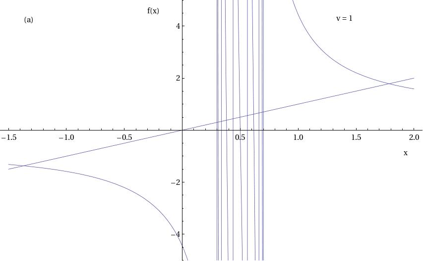
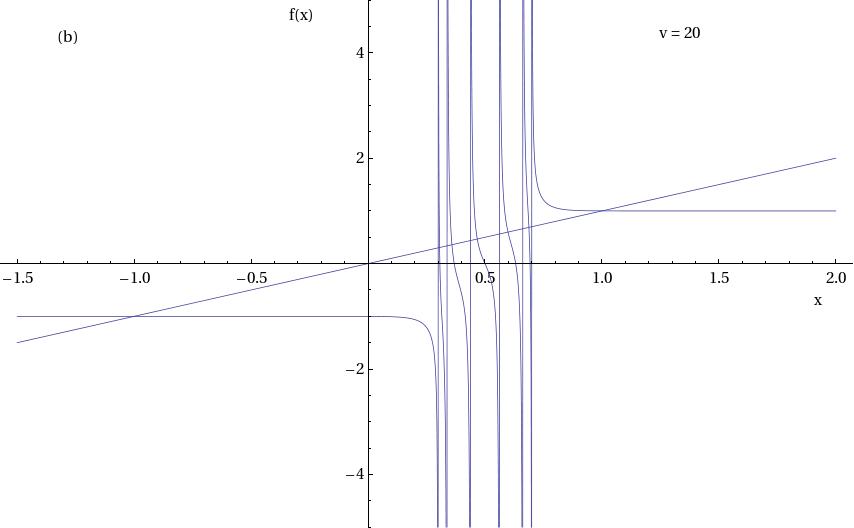
Figure 2: Graphical solution to the self-consistent equation for the self-energy in the Bose-Hubbard model for $J/V=0.1$, $\mu/V=0.5$, N = 10. The solutions (i.e. the values of $\Pi/V$ which satisfy (45)) are given by the points where the curves are crossed by the straight line; (a) $\beta V=1$, (b) $\beta V=20$

.

It is to be noticed that one of the parameters we used to plot Fig. 2, namely $j=J/V$ has been taken to be $0.1$. Such a value is quite realistic. However, it obviously means that we are in the strong coupling regime, for which the statistical linearization may lead to erroneous results. Thus, the above figures are to be understood merely as an illustration of possible solutions of (45). There is, unfortunately, no general theory which could determine whether or not the statistical linearization provides valid approximations in the strong coupling regime.

As is clearly seen from Eq. (45) and from the figures, the gap equation possesses multiple solutions. A similar situation occcurs in both QCD WQLCRS and in the superconductivity theory SSL . We plan to discuss the important and interesting question of stability of various solutions elsewhere.

V Concluding remarks

In this paper we have applied the statistical linearization technique to the stochastically quantized field equations in Euclidean setting. Three examples have been given: the quantum anharmonic oscillator, the real scalar $\phi^{4}$ theory, and the Bose-Hubbard model. In all three cases a self-consistent non-perturbative expression for the temperature-dependent self-energy has been provided. Only the simplest, Gaussian, version of the linearization technique have been employed. As a matter of fact, the statistical linearization methods are very rich. At least two ways can be used in order to improve the acuracy of results. Firstly, one can apply the so-called higher-order linearization Iyengar ; RS ; Socha . Within that approach, one replaces non-linear terms in the field equations by a new dependent variable, which satisfies its own (complicated) differential equation; the latter is then linearized by error minimization. That method is somewhat analogous to, but not identical with, the breaking of the Schwinger-Dyson (or, analogously, BBGKY) hierarchy of the integro-differential equations for the correlation functions. Secondly, one can also employ the so-called “equivalent non-linearization” Caughey2 ; RS ; Socha approach in which the original non-linear equations are replaced by simpler (though still non-linear) equations with known statistical properties of solutions. Work is in progress on application of both those techniques in the physics of cold gases, quantum electrodynamics and quantum optics.

References

- (1) G. Parisi and Y.-S. Wu, Sci. Sinica 24 (1981) 483.
- (2) P.H. Damgaard and H. Hüffel, Phys. Rep. 152 (1987) 227.
- (3) M. Namiki, Stochastic Quantization, Lectures Notes in Physics (Springer, Berlin 1992).
- (4) G. Menezes and N.F. Svaiter, Physica A 374 (2007) 617.
- (5) H. Hüffel and H. Rumpf, Phys. Lett. B 148 (1984) 104.
- (6) E. Gozzi, Phys. Lett. B 150 (1985) 119.
- (7) H. Hüffel and H. Nakazato, Mod. Phys. Lett. A9 (1994) 2953-2966
- (8) K. Yuasa and H. Nakazato, unpublished (arXiv:hep-th/9610209v1)
- (9) P.A. Amundsen and P.H. Damgaard, Phys. Rev. D 29, 323 (1984)
- (10) A. Berard, Y. Grandati and P. Grange, Inter. J. Theor. Phys. 36, 613 (1997)
- (11) A. Berard and Y. Grandati, Inter. J. Theor. Phys. 38, 623 (1999)
- (12) A. Berard and Y. Grandati, Inter. J. Theor. Phys. 38, 2535 (1999)
- (13) R.C. Booton, IRE Transactions on Circuit Theory 1 (1954) 32
- (14) I.E. Kazakov, Approximate Methods for the Statistical Analysis of Nonlinear Systems (Trudy VVIA 394, 1954)
- (15) T.K. Caughey. J. Acoust. Soc. Am. 35 (1963) 1706
- (16) T.S. Atalik and S. Utku, Earthquake Eng. Struct. Dyn., 4, (1976) 411.
- (17) H.M. Ito, J. Stat. Phys. 37 (1984) 653
- (18) J.B. Roberts and P.D. Spanos, Random Vibrations and Statistical Linearization (Dover, Mineola 2003)
- (19) L. Socha, Linearization Methods for Stochastic Dynamic Systems (Springer, Berlin 2007)
- (20) M. Namiki and M. Kanenaga, Phys. Lett. A 249, (1998) 13
- (21) T. Altherr, Phys. Lett. B 238 (1990) 360
- (22) M. Le Bellac, Thermal Field Theory (Cambridge University Press 1996)
- (23) I.T. Drummond, R.R. Hogan, P.V. Landshoff, and A. Rebhan, Nucl. Phys. B 524 (1998) 579
- (24) J.-P. Blaizot, W. Iancu and U. Reinosa, Nucl.Phys. A 736 (2004) 149
- (25) U. Kraemmer and A. Rebhan, Rep. Prog. Phys. 67 (2004) 351
- (26) V.M. Mostepanenko and N.N. Trunov, Casimir Effect and Its Application (Oxford Science Publication 1997)
- (27) E. Delabaere, in: Algorithms Seminar 2001-2002, F. Chyzak ed., (INRIA 2003), http://algo.inria.fr/seminars
- (28) J.J.G. Moreta (unpublished), http://www.gsjournal.net/old/stham/moreta30.pdf
- (29) N.N. Lebedev, Special Functions and Their Applications, edited by R.A. Silverman (Dover, New York 1972)
- (30) M. Abramowitz and I. Stegun (eds.) Handbook of Mathematical Functions (Dover, New York 1972)
- (31) R.N. Iyengar, Int. J. Non-Linear Mech. 23 (1988) 385
- (32) T.K. Caughey, Probabilistic Engineering Mechanics 1 (1986) 2
- (33) K.-L.Wang, S.-X. Qin, Y.-X. Liu, L. Chang, C.D. Roberts, and S.M. Schmidt Phys. Rev. D 86, 114001 (2012)
- (34) P.N. Spathis, M.P. Soerensen and N. Lazarides, Phys. Rev. B 45, 7360 (1992)