December 2012

ABSTRACT

Physical properties of the quantum gravitational vacuum state are explored by solving a lattice version of the Wheeler-DeWitt equation. The constraint of diffeomorphism invariance is strong enough to uniquely determine part of the structure of the vacuum wave functional in the limit of infinitely fine triangulations of the three-sphere. In the large fluctuation regime the nature of the wave function solution is such that a physically acceptable ground state emerges, with a finite non-perturbative correlation length naturally cutting off any infrared divergences. The location of the critical point in Newton’s constant $G_{c}$, separating the weak from the strong coupling phase, is obtained, and it is inferred from the general structure of the wave functional that fluctuations in the curvatures become unbounded at this point. Investigations of the vacuum wave functional further suggest that for weak enough coupling, $G<G_{c}$, a pathological ground state with no continuum limit appears, where configurations with small curvature have vanishingly small probability. One would then be lead to the conclusion that the weak coupling, perturbative ground state of quantum gravity is non-perturbatively unstable, and that gravitational screening cannot be physically realized in the lattice theory. The results we find tend to be in general agreement with the Euclidean lattice gravity results, and would suggest that the Lorentzian and Euclidean lattice formulations of gravity ultimately describe the same underlying non-perturbative physics.

1 Introduction

We have argued in previous work that the correct identification of the true ground state for quantum gravitation necessarily requires the introduction of a consistent nonperturbative cutoff, followed by the construction of the continuum limit in accordance with the methods of the renormalization group. To this day the only known way to introduce such a non-perturbative cutoff reliably in quantum field theory is via the lattice formulation. A wealth of results have been obtained over the years using the Euclidean lattice formulation, which allows the identification of the physical ground state and the accurate calculations of gravitational scaling dimensions, relevant for the scale dependence of Newton’s constant in the universal scaling limit.

In this work we will focus instead on the Hamiltonian approach to gravity, which assumes from the very beginning a metric with Lorentzian signature. Recently a Hamiltonian lattice formulation was written down based on the Wheeler-DeWitt equation, where the gravity Hamiltonian is expressed in the metric-space representation. Specifically, in [1, 2] a general discrete Wheeler-DeWitt equation was given for pure gravity, based on the simplicial lattice transcription of gravity formulated by Regge and Wheeler. Here we extend the work initiated in [1, 2] to the physical case of $3+1$ dimensions, and show how nonperturbative vacuum solutions to the lattice Wheeler-DeWitt equations can be obtained for arbitrary values of Newton’s constant $G$. The procedure we follow is similar to what was done earlier in $2+1$ dimensions. We solve the lattice equations exactly for several finite and regular triangulations of the three-sphere, and then extend the result to an arbitrarily large number of tetrahedra. We then argue that for large enough volumes the exact lattice wave functional is expected to depend on geometric quantities only, such as the total volumes and the total integrated curvature. In this process, the regularity condition on the solutions of the wave equation at small volumes plays an essential role in constraining the form of the vacuum wave functional. A key ingredient in the derivation of the results is of course the local diffeomorphism invariance of the Regge-Wheeler lattice formulation.

From the structure of the resulting wave function a number of potentially useful physical results can be obtained. First one observes that the non-perturbative correlation length is found to be finite for sufficiently large $G$. At the critical point $G=G_{c}$, which we determine exactly from the structure of the wave function, fluctuations in the curvature become unbounded, thus signaling a divergence in the non-perturbative gravitational correlation length. We argue that such a result can be viewed as consistent with the existence of a non-trivial ultraviolet fixed point (or a phase transition in statistical field theory language) in $G$. Furthermore, the behavior of the theory in the vicinity of such a fixed point is expected to determine, through standard renormalization group arguments, the scale dependence of the gravitational coupling in the vicinity of the ultraviolet fixed point.

An outline of the paper is as follows. In Sec. 2, as a background to the rest of the paper, we briefly summarize the formalism of canonical gravity. At this stage the continuum Wheeler-DeWitt equation with its invariance properties are introduced. We then briefly outline the general properties of the lattice Wheeler-DeWitt equation presented in our previous work, and in Sec. 3 we make explicit various quantities that appear in it. Here we also emphasizes the important role of continuous lattice diffeomorphism invariance in the Regge theory, as it applies to the case of $3+1$-dimensional gravity. Sec. 4 focuses on basic scaling properties of the lattice equations and useful choices for the lattice coupling constants, with the aim of giving a more transparent form to the results obtained later. Sec. 5 presents an outline of the method of solution for the lattice equations, which are later discussed in some detail for a number of regular triangulations of the three-sphere. Then a general form of the wave function is given that covers all previous discrete cases, and thus allows a study of the infinite volume limit. Sec. 6 discusses the issue of how to define an average volume and thus an average lattice spacing, an essential ingredient in the interpretation of the results given later. Sec. 7 discusses modifications of the wave function solution obtained when the explicit curvature term in the Wheeler-DeWitt equation is added. Later a partial differential equation for the wave function is derived in the curvature and volume variables. General properties of the solution to this equation are discussed in Sec. 8. Sec. 9 contains a brief summary of the results obtained so far.

2 Continuum and Discrete Wheeler-DeWitt Equation

Our work deals with the canonical quantization of gravity, and we begin here therefore with a very brief summary of the classical canonical formalism [3] as formulated by Arnowitt, Deser and Misner [4]. Many of the results found in this section are not new, but nevertheless it will be useful, in view of later applications, to recall here the main results and provide suitable references for expressions used in the following sections. Here $x^{i}$ $(i=1,2,3)$ will be coordinates on a three-dimensional manifold, and indices will be raised and lowered with $g_{ij}({\bf x})$ $(i,j=1,2,3)$, the three-metric on the given spacelike hypersurface. As usual $g^{ij}$ denotes the inverse of the matrix $g_{ij}$. Our conventions are such that the space-time metric has signature $-+++$, that ${}^{4}\!R$ is non-negative in a space-time containing normal matter, and that ${}^{3}\!R$ is positive in a 3-space of positive curvature.

One goes from the classical to the quantum description of gravity by promoting the metric $g_{ij}$, the conjugate momenta $\pi^{ij}$, the Hamiltonian density $H$ and the momentum density $H_{i}$ to quantum operators, with ${\hat{g}}_{ij}$ and ${\hat{\pi}}^{ij}$ satisfying canonical commutation relations. Then the classical constraints select physical states $|\Psi\rangle$, such that in the absence of sources

$${\hat{H}}\,|\Psi\rangle\,=\,0\;\;\;\;\;\;{\hat{H}}_{i}\,|\Psi\rangle\,=\,0\;\;,$$ (1)

whereas in the presence of sources one has more generally

$${\hat{T}}\,|\Psi\rangle\,=\,0\;\;\;\;\;\;{\hat{T}}_{i}\,|\Psi\rangle\,=\,0\;\;,$$ (2)

with ${\hat{T}}$ and ${\hat{T}}_{i}$ describing matter contributions that can be added to ${\hat{H}}$ and ${\hat{H}}_{i}$. As is the case in nonrelativistic quantum mechanics, one can choose different representations for the canonically conjugate operators ${\hat{g}}_{ij}$ and ${\hat{\pi}}^{ij}$. In the functional metric representation one sets

$${\hat{g}}_{ij}({\bf x})\;\rightarrow\;g_{ij}({\bf x})\;\;\;\;\;\;\;{\hat{\pi}}^{ij}({\bf x})\;\rightarrow\;-i\hbar\cdot 16\pi G\cdot{\delta\over\delta g_{ij}({\bf x})}\;.$$ (3)

Then quantum states become wave functionals of the three-metric $g_{ij}({\bf x})$,

$$|\Psi\rangle\;\rightarrow\;\Psi\,[g_{ij}({\bf x})]\;.$$ (4)

The constraint equations in Eq. (2) then become the Wheeler-DeWitt equation [5, 6]

$$\left\{-\,16\pi G\cdot G_{ij,kl}\,{\delta^{2}\over\delta g_{ij}\,\delta g_{kl}}\,-\,{1\over 16\pi G}\,\sqrt{g}\,\left(\,{}^{3}\!R\,-\,2\lambda\,\right)\,+\,{\hat{H}}^{\phi}\right\}\;\Psi[g_{ij}({\bf x})]\,=\,0\;,$$ (5)

and the momentum constraint equation listed below. In Eq. (5) $G_{ij,kl}$ is the inverse of the DeWitt supermetric,

$$G_{ij,kl}\,=\,\textstyle{1\over 2}\displaystyle\,g^{-1/2}\left(g_{ik}g_{jl}+g_{il}g_{jk}\,-\,g_{ij}g_{kl}\right)\;\;.$$ (6)

The three-dimensional DeWitt supermetric itself is given by

$$G^{ij,kl}\,=\,\textstyle{1\over 2}\displaystyle\,\sqrt{g}\,\left(g^{ik}g^{jl}+g^{il}g^{jk}\,-\,2\,\,g^{ij}g^{kl}\right)\;\;.$$ (7)

In the metric representation the diffeomorphism constraint reads

$$\left\{2\,i\,g_{ij}\,\nabla_{k}\,{\delta\over\delta g_{jk}}\,+\,{\hat{H}}^{\phi}_{i}\right\}\;\Psi[g_{ij}({\bf x})]\,=\,0\;,$$ (8)

where ${\hat{H}}^{\phi}$ and ${\hat{H}}^{\phi}_{i}$ again are possible matter contributions. In the following, we shall set both of these to zero as we will focus here almost exclusively on the pure gravitational case. Then the last contraint represents the necessary and sufficient condition that the wave functional $\psi[g]$ be an invariant under coordinate transformations [7].

We note here that in the continuum one expects the commutator of two Hamiltonian constraints to be related to the diffeomorphism constraint. In the following we will, for the time being, overlook this rather delicate issue, and focus our efforts instead mainly on the solution of the explicit (lattice) Hamiltonian constraint of Eq. (15). It should nevertheless be possible to revisit this important issue at a later stage, once an exact, or approximate, candidate expression for the wave functional is found. The key issue at that stage will then be if the lattice wave functional satisfies all physical requirements, including the momentum constraint, in a suitable lattice scaling limit wherein the (average) lattice spacing is much smaller than a suitable physical scale, such as the scale of the local curvature, or some other sort of agreeable physical correlation length. For a more in-depth discussion of the analogous problem in $2+1$ dimensions we refer the reader to our previous work [2], where an explicit form for the candidate wave functional was eventually given in terms of manifestly invariant quantities such as areas and curvatures.

We should also mention here that a number of rather basic issues need to be considered before one can gain a consistent understanding of the full content of the theory [see, for example, [9, 10, 12, 13, 14]]. These include potential problems with operator ordering, and the specification of a suitable Hilbert space, which entails a choice for the norm of wave functionals, for example in the Schrödinger form

$$\lVert\Psi\rVert^{2}\,=\,\int d\mu[g]\;\Psi^{*}[g_{ij}]\;\Psi[g_{ij}]\;,$$ (9)

where $d\mu[g]$ is the appropriate (DeWitt) functional measure over the three-metric $g_{ij}$. In this work we will attempt to address some of those issues, as they will come up within the relevant calculations.

In this paper the starting point will be the Wheeler-DeWitt equation for pure gravity in the absence of matter, Eq. (5),

$$\left\{\,-\,(16\pi G)^{2}\,G_{ij,kl}({\bf x})\,{\delta^{2}\over\delta g_{ij}({\bf x})\,\delta g_{kl}({\bf x})}\,-\,\sqrt{g({\bf x})}\;\left(\;{}^{3}\!R({\bf x})\,-\,2\lambda\,\right)\,\right\}\;\Psi[g_{ij}({\bf x})]\,=\,0\;,$$ (10)

combined with the diffeomorphism constraint of Eq. (8),

$$\left\{\,2\,i\,g_{ij}({\bf x})\,\nabla_{k}({\bf x})\,{\delta\over\delta g_{jk}({\bf x})}\,\right\}\;\Psi[g_{ij}({\bf x})]\,=\,0\;.$$ (11)

Both of these equations express a constraint on the state $|\Psi\rangle$ at every ${\bf x}$. It is then natural to view Eq. (10) as made up of three terms, the first one identified as the kinetic term for the metric degrees of freedom, the second one involving $-\,\sqrt{g}\,{}^{3}\!R$ and thus seen as a potential energy contribution (of either sign, due to the nature of the 3-curvature ${}^{3}\!R$), and finally the cosmological constant term proportional to $+\,\lambda\,\sqrt{g}$ acting as a mass-like term. The kinetic term contains a Laplace-Beltrami-type operator acting on the 6-dimensional Riemannian manifold of positive definite metrics $g_{ij}$, with $G_{ij,kl}$ acting as its contravariant metric [7]. As shown in the quoted reference, the manifold in question has hyperbolic signature $-+++++$, with pure dilations of $g_{ij}$ corresponding to timelike displacements within this manifold of metrics.

Next we turn to the lattice theory. Here we will generally follow the procedure outlined in [1] and discretize the continuum Wheeler-DeWitt equation directly, a procedure that makes sense in the lattice formulation, as these equations are still formulated in terms of geometric objects, for which the Regge theory is very well suited. It is known that on a simplicial lattice [16, 17, 18, 19, 20, 21, 22] (see for example [23] for a more detailed presentation of the Regge-Wheeler lattice formulation) deformations of the squared edge lengths are linearly related to deformations of the induced metric. In a given simplex $\sigma$, take coordinates based at a vertex $0$, with axes along the edges emanating from $0$. Then the other vertices are each at unit coordinate distance from $0$ (see Figure 1 as an example of this labeling for a tetrahedron). With this choice of coordinates, the metric within a given simplex is

$$g_{ij}(\sigma)\,=\,\textstyle{1\over 2}\displaystyle\,\left(l_{0i}^{2}+l_{0j}^{2}-l_{ij}^{2}\right)\;\;.$$ (12)

We note that in the following discussion only edges and volumes along the spatial directions are involved. Then by varying the squared volume of a given simplex $\sigma$ in $d$ dimensions to quadratic order in the metric (in the continuum), or in the squared edge lengths belonging to that simplex (on the lattice), one is led to the identification [24, 25]

$$G^{ij}(l^{2})\,=\,-\;d!\;\sum_{\sigma}\;{1\over V(\sigma)}\;{\partial^{2}\;V^{2}(\sigma)\over\partial l^{2}_{i}\;\partial l^{2}_{j}}\;\;,$$ (13)

where the quantity $G^{ij}(l^{2})$ is local, since the sum over $\sigma$ only extends over those simplices which contain either the $i$ or the $j$ edge. In the formulation of [1] it will be adequate to limit the sum in Eq. (13) to a single tetrahedron, and define the quantity $G^{ij}$ for that tetrahedron. Then, in schematic terms, the lattice Wheeler-DeWitt equation for pure gravity takes on the form

$$\left\{\,-\,(16\pi G)^{2}\,G_{ij}(l^{2})\,{\partial^{2}\over\partial l^{2}_{i}\,\partial l^{2}_{j}}\,-\,\sqrt{g(l^{2})}\;\left[\;{}^{3}\!R(l^{2})\,-\,2\lambda\;\right]\;\right\}\,\Psi[\,l^{2}\,]\,=\,0\;\;,$$ (14)

with $G_{ij}(l^{2})$ the inverse of the matrix $G^{ij}(l^{2})$ given above. The range of summation over the indices $i$ and $j$ and the appropriate expression for the scalar curvature will be made explicit later in Eq. (15).

It is clear that Eqs. (5) or (14) express a constraint at each “point” in space. Indeed, the first term in Eq. (14) contains derivatives with respect to edges $i$ and $j$ connected by a matrix element $G_{ij}$ which is nonzero only if $i$ and $j$ are close to each other and thus nearest neighbor. One expects therefore that the first term can be represented by a sum of edge contributions, all from within one ($d-1$)-simplex $\sigma$ (a tetrahedron in three dimensions). The second term containing ${}^{3}\!R(l^{2})$ in Eq. (14) is also local in the edge lengths: it only involves those edge lengths which enter into the definition of areas, volumes and angles around the point ${\bf x}$. The latter is therefore described, through the deficit angle $\delta_{h}$, by a sum over contributions over all ($d-3$)-dimensional hinges (edges in 3+1 dimensions) $h$ attached to the simplex $\sigma$. This then leads in three dimensions to a more explicit form of Eq. (14)

$$\left\{\,-\,(16\pi G)^{2}\sum_{i,j\subset\sigma}\,G_{ij}\,(\sigma)\,{\partial^{2}\over\partial l^{2}_{i}\,\partial l^{2}_{j}}\,-\,2\,n_{\sigma h}\;\sum_{h\subset\sigma}\,l_{h}\,\delta_{h}\,+\,2\lambda\;V_{\sigma}\,\right\}\,\Psi[\,l^{2}\,]\,=\,0\;\;.$$ (15)

In the above expression $\delta_{h}$ is the deficit angle at the hinge (edge) $h$, $l_{h}$ the corresponding edge length, and $V_{\sigma}=\sqrt{g(\sigma)}$ the volume of the simplex (tetrahedron in three spatial dimensions) labeled by $\sigma$. The matrix $G_{ij}\,(\sigma)$ is obtained either from Eq. (13) or from the lattice transcription of Eq. (6)

$$G_{ij,kl}\,(\sigma)\,=\,\textstyle{1\over 2}\displaystyle\,g^{-1/2}(\sigma)\,\left[\,g_{ik}(\sigma)\,g_{jl}(\sigma)+g_{il}(\sigma)\,g_{jk}(\sigma)-\,g_{ij}(\sigma)\,g_{kl}(\sigma)\,\right]\;,$$ (16)

with the induced metric $g_{ij}\,(\sigma)$ within a simplex $\sigma$ given in Eq. (12). Note that the combinatorial factor $n_{\sigma h}$ gives the correct normalization for the curvature term, since the latter has to give the lattice version of $\int\sqrt{g}\;{}^{3}\!R=2\sum_{h}\delta_{h}l_{h}$ when summed over all simplices $\sigma$. One can see then that the inverse of $n_{\sigma h}$ counts the number of times the same hinge appears in various neighboring simplices, and depends therefore on the specific choice of underlying lattice structure. The lattice Wheeler-DeWitt equation given in Eq. (15) was the main result of a previous paper [1] and was studied extensively in $2+1$ dimensions in previous work [2].

3 Explicit Setup for the Lattice Wheeler-DeWitt Equation

In the following we will now focus on a three-dimensional lattice made up of a large number of tetrahedra, with squared edge lengths considered as the fundamental degrees of freedom. For ease of notation, we define $l_{01}^{2}=a,\,l_{12}^{2}=b,\,l_{02}^{2}=c,\,l_{03}^{2}=d,\,l_{13}^{2}=e,\,l_{23}^{2}=f$. For the tetrahedron labeled as in Figure 1, we have

$$g_{11}\,=\,a\,,\;\;\;\;g_{22}\,=\,c\,,\;\;\;g_{33}\,=\,d\,,$$ (17)

$$g_{12}\,=\,\frac{1}{2}(a\,+\,c\,-\,b)\,,\;\;\;g_{13}\,=\,\frac{1}{2}(a\,+\,d\,-\,e)\,,\;\;\;g_{23}\,=\,\frac{1}{2}(c\,+\,d\,-\,f)\;,$$ (18)

and its volume $V$ is given by

$$V^{2} = \;\frac{1}{144}[\,af(-a-f+b+c+d+e)\,+\,bd(-b-d+a+c+e+f)\,+\,$$ (19)

$$\;\;\;\;+ ce(-c-e+a+b+d+f)\,-\,abc\,-\,ade\,-\,bef\,-\,cdf]\;.$$

The matrix $G^{ij}$ is then given by

$$G^{ij}\,=\,-\,\frac{1}{24V}\left(\begin{matrix}-2f&e+f-b&b+f-e&d+f-c&c+f-d&p\cr e+f-b&-2e&b+e-f&d+e-a&q&a+e-d\cr b+f-e&b+e-f&-2b&r&b+c-a&a+b-c\cr d+f-c&d+e-a&r&-2d&c+d-f&a+d-e\cr c+f-d&q&b+c-a&c+d-f&-2c&a+c-b\cr p&a+e-d&a+b-c&a+d-e&a+c-b&-2a\end{matrix}\right)\;,$$ (20)

where the three quantities $p$, $q$ and $r$ are defined as

$$p=-2a-2f+b+c+d+e,\;\;\;q=-2c-2e+a+b+d+f,\;\;\;r=-2b-2d+a+c+e+f\;.$$ (21)

To obtain $G_{ij}$ one can then either invert the above expression, or evaluate

$$G_{ij,kl}\,=\,\frac{1}{2\sqrt{g}}(g_{ik}\,g_{jl}\,+\,g_{il}\,g_{jk}\,-\,g_{ij}\,g_{kl}),$$ (22)

and later replace derivatives with respect to the metric by derivatives with respect to the squared edge lengths, as in ${\partial\over\partial\,g_{11}}={\partial\over\partial\,a}\,+\,{\partial\over\partial\,b}\,+\,{\partial\over\partial\,e}$ etc. One finds [1] that the matrix representing the coefficients of the derivatives with respect to the squared edge lengths is the same as the inverse of $G^{ij}$, a result that provides a nontrivial confirmation of the correctness of the Lund-Regge result of Eq. (13). Then in $3+1$ dimensions, the discrete Wheeler-DeWitt equation is

$$\left\{\,-\,(16\pi G)^{2}\,G_{ij}\,{\partial^{2}\over\partial s_{i}\partial s_{j}}\,-\,2\,n_{\sigma h}\,\sum_{h}\sqrt{s_{h}}\,\delta_{h}\,+\,2\lambda\,V\right\}\Psi[\,s\,]\,=\,0\;,$$ (23)

where the sum is over hinges (edges) $h$ in the tetrahedron, and $V$ the volume of the given tetrahedron. Note that the above represents one equation for every tetrahedron on the lattice. Thus if the lattice contains $N_{3}$ tetrahedra, there will be $N_{3}$ coupled equations that will need to be solved in order to determine $\Psi[s]$. Note also the mild nonlocality of the equation in that the curvature term, through the deficit angles, involves edge lengths from neighboring tetrahedra. Of course, in the continuum the derivatives also give some very mild nonlocality. Figure 2 gives a pictorial representation of lattices that can be used for numerical studies of quantum gravity in 3+1 dimensions.

Figure 1: A tetrahedron with labels.

Figure 2: A small section of a suitable spatial lattice for quantum gravity in $3+1$ dimensions.

In the following we will be concerned at some point with various discrete, but generally regular, triangulations of the three-sphere [26, 27]. These were already studied in some detail within the framework of the Regge theory in [20], where in particular the 5-cell $\alpha_{4}$, the 16-cell $\beta_{4}$ and the 600-cell regular polytopes (as well as a few others) were considered in some detail. For a very early application of these regular triangulations to general relativity see [28].

We shall not dwell here on a well-known key aspect of the Regge-Wheeler theory, which is the presence of a continuous, local lattice diffeomorphism invariance, whose main aspects in regards to its relevance for the $3+1$ formulation of gravity were already addressed in some detail in various works, both in the framework of the lattice weak field expansion [16, 1], and beyond it [22, 29]. Here we will limit ourselves to some brief remarks on how this local invariance manifests itself in the $3+1$ formulation, and, in particular, in the case of the discrete triangulations of the sphere studied later on in this paper. In general, lattice diffeomorphisms in the Regge-Wheeler theory correspond to local deformations of the edge lengths about a vertex, which leave the local geometry physically unchanged, the latter being described by the values of local lattice operators corresponding to local volumes and curvatures [16, 22, 29]. The case of flat space (curvature locally equal to zero) or near-flat space (curvature locally small) is obviously the simplest to analyze [29]: by moving the location of the vertices around on a smooth manifold one can find different assignments of edge lengths representing locally the same flat, or near-flat, geometry. It is then easy to show that one obtains a $d\cdot N_{0}$-parameter family of local transformations for the edge lengths, as expected for lattice diffeomorphisms. For the present case, the relevant lattice diffeomorphisms are the ones that apply to the three-dimensional, spatial theory. The reader is referred to [30] and, more recently, [1] for their explicit form within the framework of the lattice weak field expansion.

With these observations in mind, we can now turn to a discussion of the solution method for the lattice Wheeler-DeWitt equation in $3+1$ dimensions. One item that needs to be brought up at this point is the proper normalization of various terms (kinetic, cosmological and curvature) appearing in the lattice equation of Eqs. (15) and (23). For the lattice gravity action in $d$ dimensions one has generally the following correspondence

$$\int d^{d}x\,\sqrt{g}\;\;\;\longleftrightarrow\;\;\;\sum_{\sigma}\,V_{\sigma}\;,$$ (24)

where $V_{\sigma}$ is the volume of a simplex; in three dimensions it is simply the volume of a tetrahedron. The curvature term involves deficit angles in the discrete case,

$$\textstyle{1\over 2}\displaystyle\,\int\,d^{d}x\,\sqrt{g}\,R\;\;\;\longleftrightarrow\;\;\;\sum_{h}\,V_{h}\,\delta_{h}\;,$$ (25)

where $\delta_{h}$ is the deficit angle at the hinge $h$, and $V_{h}$ the associated “volume of a hinge” [15]. In four dimensions the latter is the area of a triangle (usually denoted by $V_{h}$), whereas in three dimensions it is simply given by the length $l_{h}$ of the edge labeled by $h$. In this work we will focus almost exclusively on the case of $3+1$ dimensions; consequently the relevant formulas will be Eqs. (24) and (25) for dimension $d=3$.

The continuum Wheeler-DeWitt equation is local, as can be seen from Eq. (10). One can integrate the Wheeler-DeWitt operator over all space and obtain

$$\left\{-\,\left(16\pi\,G\right)^{2}\,\int d^{3}x\;{\bf\Delta}(g)\,+2\lambda\int d^{3}x\,\sqrt{g}-\int d^{3}x\,\sqrt{g}\,R\,\right\}\,\Psi=0\;,$$ (26)

with the super-Laplacian on metrics defined as

$${\bf\Delta}(g)\;\equiv\;G_{ij,kl}({\bf x})\;{\delta^{2}\over\delta g_{ij}({\bf x})\,\delta g_{kl}({\bf x})}\;.$$ (27)

We have seen before that in the discrete case one has one local Wheeler-DeWitt equation for each tetrahedron [see Eqs. (14) and (15)], which can be written as

$$\left\{\,-\,(16\pi\,G)^{2}\;{\bf\Delta}(l^{2})-\,\kappa\,\sum_{h\subset\sigma}\delta_{h}\,l_{h}+2\,\lambda\,V_{\sigma}\,\right\}\,\Psi=0\;,$$ (28)

where now ${\bf\Delta}(l^{2})$ is the lattice version of the super-Laplacian, and we have set for convenience $\kappa=2\,n_{\sigma\,h}$. As we shall see below, for a regular lattice of fixed coordination number, $\kappa$ is a constant and does not depend on the location on the lattice. In the above expression ${\bf\Delta}(l^{2})$ is a discretized form of the covariant super-Laplacian, acting locally on the space of $s=l^{2}$ variables,

$${\bf\Delta}(l^{2})\;\equiv\;G_{ij}\;{\partial^{2}\over\partial s_{i}\partial s_{j}}\;,$$ (29)

with the matrix $G^{ij}$ given explicitly in Eq. (20). Note that the curvature term involves six deficit angles $\delta_{h}$, associated with the six edges of a tetrahedron.

Now, the local lattice Wheeler-DeWitt equation of Eq. (23) applies to a single given tetrahedron (labeled here by $\sigma$), with one equation to be satisfied at each tetrahedron on the lattice. At this point some simple additional checks can be performed. For example, one can also construct the total Hamiltonian by simply summing over all tetrahedra, which leads to

$$\left\{-\,(16\pi\,G)^{2}\,\sum_{\sigma}\,{\bf\Delta}(l^{2})\,+\,2\,\lambda\sum_{\sigma}V_{\sigma}\,-\,\kappa\,\sum_{\sigma}\sum_{h\subset\sigma}\,l_{h}\,\delta_{h}\right\}\,\Psi=0\;.$$ (30)

The above expression represents therefore an integral over Hamiltonian constraints with unit density weights. Note that indeed the second term involves the total lattice volume (the lattice analog of $\int d^{3}x\,\sqrt{g}$), and the third one contains, as expected, the total lattice curvature (the lattice analog of $\int d^{3}x\,\sqrt{g}\,R$)[15].

Summing over all tetrahedra $(\sigma)$ is different from summing over all hinges $(h)$, and the above equation is equivalent to

$$\left\{-\,(16\pi\,G)^{2}\,\sum_{\sigma}{\bf\Delta}(l^{2})\,+\,2\,\lambda\sum_{\sigma}V_{\sigma}\,-\,\kappa\,q\,\sum_{h}\,l_{h}\,\delta_{h}\right\}\,\Psi=0\;,$$ (31)

where $q$ here is the lattice coordination number. The latter is determined by how the lattice is put together (which vertices are neighbors to each other, or, equivalently, by the so-called incidence matrix). Here $q$ is therefore the number of neighboring simplexes that share a given hinge (edge). For a flat triangular lattice in 2d $q=6$, whereas for the regular triangulations of $S^{3}$ we will be considering below one has $q=3,\,4,\,5$. For more general, irregular triangulations $q$ might change locally throughout the lattice. In this case it is more meaningful to talk about an average lattice coordination number $<\!q\!>$ [19]. For proper normalization in Eq. (30) one requires the three-dimensional version of Eqs. (24) and (25), which fixes the overall normalization of the curvature term

$$\kappa\,\equiv\,2\,n_{\sigma\,h}\,=\,{2\over q}\;,$$ (32)

thus determining the relative weight of the local volume and curvature terms. At this point it seems worth emphasizing that from now on we will focus exclusively on the set of coupled local lattice Wheeler-DeWitt equations, given explicitly in Eqs. (23) or (28), with one equation for each lattice tetrahedron.

4 Choice of Coupling Constants

We will find it convenient, in analogy to what is commonly done in the Euclidean lattice theory of gravity, to factor out an overall irrelevant length scale from the problem, and set the (unscaled) cosmological constant equal to one [20]. Indeed, recall that the Euclidean path integral statistical weight always contains a factor $P(V)\propto\exp(-\lambda_{0}V)$, where $V=\int\sqrt{g}$ is the total volume on the lattice, and $\lambda_{0}$ is the unscaled cosmological constant. A simple global rescaling of the metric (or edge lengths) then allows one to entirely reabsorb this $\lambda_{0}$ into the local volume term. The choice $\lambda_{0}=1$ then trivially fixes this overall scale once and for all. Since $\lambda_{0}=2\lambda/16\pi G$, one then has $\lambda=8\pi G$ in this system of units. In the following we will also find it convenient to introduce a scaled coupling $\tilde{\lambda}$ defined as

$$\tilde{\lambda}\;\equiv\;{\lambda\over 2}\left({1\over 16\pi G}\right)^{2}\;.$$ (33)

Then for $\lambda_{0}=1$ (in units of the $UV$ cutoff or, equivalently, in units of the fundamental lattice spacing) one has $\tilde{\lambda}=1/64\pi G$.

Two further notational simplifications will be useful in the following. The first one is introduced in order to avoid lots of factors of $16\pi$ in many of the formulas. So from now on we shall write $G$ as a shorthand for $16\pi\,G$,

$$16\pi\,G\longrightarrow G\;.$$ (34)

In this new notation one has $\lambda=G/2$ and $\tilde{\lambda}=1/4G$. The above notational choices then lead to a more streamlined representation of the Wheeler-DeWitt equation, namely

$$\left\{-\,{\bf\Delta}\,+\,{1\over G}\,\sqrt{g}\,-\,{1\over G^{2}}\,\sqrt{g}\;{}^{3}\!R\,\right\}\,\Psi=0\;.$$ (35)

Note that we have arranged things so that now the kinetic term (the term involving the Laplacian) has a unit coefficient. Then in the extreme strong coupling limit ($G\rightarrow\infty$) the kinetic term is the dominant one, followed by the volume (cosmological constant) term (using the facts about $\tilde{\lambda}$ given above) and, finally, by the curvature term. Consequently, at least in a first approximation, the curvature $R$ term can be neglected compared to the other two terms, in this limit.

A second notational choice will later be dictated by the structure of the wave function solutions, which often involve numerous factors of $\sqrt{G}$. It will therefore be useful to define a new coupling $g$ as

$$g\;\equiv\;\sqrt{G}\;,$$ (36)

so that $\tilde{\lambda}=4/g^{2}$ (the latter $g$ should not be confused with the square root of the determinant of the metric).

5 Outline of the General Method of Solution

The previous discussion shows that in the strong coupling limit (large $G$) one can, at least in a first approximation, neglect the curvature term, which will then be included at a later stage. This simplifies the problem considerably, as it is the curvature term that introduces complicated interactions between neighboring simplices.

Here the general procedure for finding a solution will be rather similar to what was done in $2+1$ dimensions, as the formal issues in obtaining a solution are not dramatically different. First an exact solution is found for equilateral edge lengths $s$. Later this solution is extended to determine whether it is consistent to higher order in the weak field expansion, where one writes for the squared edge lengths the expansion

$$l_{ij}^{2}\;=\;s\left(1\,+\,\epsilon\,h_{ij}\right)\;,$$ (37)

with $\epsilon$ a small expansion parameter. The resulting solution for the wave function can then be obtained as a suitable power series in the $h$ variables, combined with the standard Frobenius method, appropriate for the study of quantum mechanical wave equations for suitably well-behaved potentials. In this method one first determines the correct asymptotic behavior of the solution for small and large arguments, and later constructs a full solution by writing the remainder as a power series or polynomial in the relevant variable. While this last method is rather time consuming, we have found nevertheless that in some cases (such as the single triangle in $2+1$ dimensions and the single tetrahedron in $3+1$ dimensions, described in [1] and also below), one is lucky enough to find immediately an exact solution, without having to rely in any way on the weak field expansion.

More importantly, in [2] it was found that already in $2+1$ dimensions this rather laborious weak field expansion of the solution is not really necessary, for the following reason. Diffeomorphism invariance (on the lattice and in the continuum) of the theory severely restricts the form of the Wheeler-DeWitt wave function to a function of invariants only, such as total three-volumes and curvatures, or powers thereof. In other words, the wave function is found to be a function of invariants such as $\int d^{d}x\sqrt{g}$ or $\int d^{d}x\sqrt{g}\,R^{n}$ etc. (these will be listed in more detail below for the specific case of $3+1$ dimensions, where one has $d=3$ in the above expressions).

For concreteness and computational expedience, in the following we will look at a variety of three-dimensional simplicial lattices, including regular triangulations of the three-sphere $S^{3}$ constructed as convex 4-polytopes, the latter describing closed and connected figures composed of lower dimensional simplices. Here these will include the 5-cell 4-simplex or hypertetrahedron (Schläfli symbol $\{3,3,3\}$) with 5 vertices, 10 edges and 5 tetrahedra; the 16-cell hyperoctahedron (Schläfli symbol $\{3,3,4\}$) with 8 vertices, 24 edges and 16 tetrahedra; and the 600-cell hypericosahedron (Schläfli symbol $\{3,3,5\}$) with 120 vertices, 720 edges and 600 tetrahedra [26, 27]. Note that the Euler characteristic for all 4-polytopes that are topological 3-spheres is zero, $\chi=N_{0}-N_{1}+N_{2}-N_{3}=0$, where $N_{d}$ is the number of simplices of dimension $d$. We also note here that there are no known regular equilateral triangulations of the flat 3-torus in three dimensions, although very useful slightly irregular (but periodic) triangulations are easily constructed by subdividing cubes on a square lattice into tetrahedra [30].

In the following we will also recognize that there are natural sets of variables for displaying the results. One of them is the scaled total volume $x$, defined as

$$x\;\equiv\;{4\,\sqrt{2\lambda}\over q\,G}\;\sum_{\sigma}\,V_{\sigma}\;=\;{4\,\sqrt{2\lambda}\over q\,G}\;V_{tot}\;.$$ (38)

Later on we will be interested in making contact with continuum manifolds, by taking the infinite volume (or thermodynamic) limit, defined in the usual way as

$$N_{\sigma} \rightarrow \infty\;,$$

$$V_{tot} \rightarrow \infty\;,$$

$${V_{tot}\over N_{\sigma}} \rightarrow {\rm const.}\;,$$ (39)

with $N_{\sigma}\equiv N_{3}$ here the total number of tetrahedra. It should be clear that this last ratio can be used to define a fundamental lattice spacing $a_{0}$, for example via $V_{tot}/N_{\sigma}\equiv V_{\sigma}=a_{0}^{3}/6\sqrt{2}$.

The full solution of the quantum mechanical problem will, in general, require that the wave functions be properly normalized, as in Eq. (9). This will introduce at some stage wave function normalization factors ${\mathcal{N}}$, which will later be fixed by the standard rules of quantum mechanics. If the wave function were to depend on the total volume $V_{tot}$ only (which is the case in $2+1$ dimensions, but not in $3+1$), then the relevant requirement would simply be

$$\lVert\Psi\rVert^{2}\;\equiv\;\int d\mu[g]\cdot\lvert\,\Psi[g_{ij}]\,\lvert^{2}\;=\;\int_{0}^{\infty}dV_{tot}\cdot V_{tot}^{m}\cdot\lvert\,\Psi(V_{tot})\,\lvert^{2}\;=\;1\;,$$ (40)

where $d\mu[g]$ is the appropriate functional measure over the three-metric $g_{ij}$, and $m$ a positive real number representing the correct entropy weighting. But, not unexpectedly, in $3+1$ dimensions the total curvature also plays a role, so the above can only be regarded as roughly correct in the strong coupling limit (large $G$), where the curvature contribution to the Wheeler-DeWitt equation can safely be neglected. As in nonrelativistic quantum mechanics, the normalization condition in Eqs. (9) and (40) plays a crucial role in selecting out of the two solutions the one that is regular, and therefore satisfies the required wave function normalizability condition.

To proceed further, it will be necessary to discuss each lattice separately in some detail. For each lattice geometry, we will break down the presentation into two separate discussions. The first part will deal with the case of no explicit curvature term in the Wheeler-DeWitt equation. Each regular triangulation of the three-sphere will be first analyzed separately, and subjected to the required regularity conditions. Here a solution is first obtained in the equilateral case, and later promoted on the basis of lattice diffeomorphism invariance to the case of arbitrary edge lengths, as was done in [2]. Later a single general solution will be written down, involving the parameter $q$, which covers all previous triangulation cases, and thereby allows a first study of the infinite volume limit. The second part deals with the extension of the previous solutions to the case when the curvature term in the Wheeler-DeWitt equation is included. This case is more challenging to treat analytically, and the only results we have obtained so far deal with the large volume limit, for which the solution is nevertheless expected to be exact (as was the case in $2+1$ dimensions [2]).

5.1 Nature of Solutions in 3+1 Dimensions

In this work we will be concerned with the solution of the Wheeler-DeWitt equation for discrete triangulations of the three-sphere $S^{3}$. In general, for an arbitrary triangulation of a smooth closed manifold in three dimensions, one can write down the Euler equation

$$N_{0}-N_{1}+N_{2}-N_{3}=0$$ (41)

and the Dehn-Sommerville relation

$$N_{2}=2\,N_{3}\;.$$ (42)

The latter follows from the fact that each triangle is shared by two tetrahedra and each tetrahedron has four triangles, thus $2\,N_{2}=4\,N_{3}$. In addition, for the regular triangulations of the three-sphere we will be considering here, one has the additional identity

$$N_{1}={6\over q}\,N_{3}\;,$$ (43)

where $q$ is the local coordination number, defined as the number of tetrahedra meeting at an edge. For the three regular triangulations of the three-sphere we will look at one has $q=3,4,5$. The above relations then allow us to relate the number of sites ($N_{0}$) to the number of tetrahedra ($N_{3}$),

$$N_{0}=N_{3}\,\left({6\over q}-1\right)\;.$$ (44)

It will also turn out to be convenient to collect here a number of useful definitions, results and identities that apply to the regular triangulations of the three-sphere, valid strictly when all edge lengths take on the same identical value $l=\sqrt{s}$. For the total volume

$$V_{tot}\equiv\;\sum_{\sigma}V_{\sigma}\;\;\longleftrightarrow\;\;\int d^{3}x\,\sqrt{g}$$ (45)

one has

$$V_{tot}\,=\,N_{3}\,V_{\sigma}={s^{3/2}\over 6\sqrt{2}}\;N_{3}\;,$$ (46)

whereas the total curvature

$$R_{tot}\;\equiv\;2\;\sum_{h}\delta_{h}\,l_{h}\;\;\longleftrightarrow\;\;\int d^{3}x\,\sqrt{g}\,R$$ (47)

is given by

$$R_{tot}={12\,\sqrt{s}\over q}\,\left[2\,\pi-q\,\cos^{-1}\left(\textstyle{1\over 3}\displaystyle\right)\right]\,N_{3}\;.$$ (48)

The latter relationship can be inverted to give the parameter $q$ as a function of the curvature

$$q\;=\;q_{0}\,\left(1-{R_{tot}\over R_{tot}+{24\,\pi\,\sqrt{s}\over q_{0}}\;N_{3}}\right)\;,$$ (49)

and its inverse as

$$q^{-1}\;=\;q_{0}^{-1}+{R_{tot}\over 24\,\pi\,\sqrt{s}\;N_{3}}\;,$$ (50)

so that this last quantity is just linear in $R_{tot}$. A very special value for $q$ corresponds to the choice $q=q_{0}$ for which $R_{tot}=0$. For this case one has

$$q_{0}\;\equiv\;{2\,\pi\over\cos^{-1}(\textstyle{1\over 3}\displaystyle)}=5.1043\;.$$ (51)

We emphasize here again that the relationships just given above apply to the rather special case of an equilateral triangulation.

Then, summarizing all the previous discussions, the discretized Wheeler-DeWitt equation one wants to solve here in the most general case is the one given in Eqs. (23) or (28),

$$\left\{\,-\,G^{2}\sum_{i,j\subset\sigma}\,G_{ij}\,(\sigma)\,{\partial^{2}\over\partial l^{2}_{i}\,\partial l^{2}_{j}}\;-\;\kappa\;\sum_{h\subset\sigma}\,l_{h}\,\delta_{h}\;+\;2\lambda\;V_{\sigma}\,\right\}\;\psi[\,l^{2}\,]\;=\;0\;\;,$$ (52)

with parameter $\kappa$ given by

$$\kappa={2\over q}\;\;.$$ (53)

Note that Eq. (52) still represents one equation per lattice tetrahedron. Thus if the lattice is made up of $N_{3}$ tetrahedra, the problem will in general still require the solution of $N_{3}$ coupled equations of the type given in Eq. (52), involving in the most general case $N_{1}$ edge lengths. As will be discussed further below, the proposed method of solution will be quite similar to what was used earlier in $2+1$ dimensions [2], namely a combination of the weak field expansion and the Frobenius method, which in [2] gave the exact solution for the wavefunction for each lattice in the limit of large areas. If the reader is not interested here in the details of the solution for each individual lattice, then (s)he can skip the following sections and move on directly to Sec. (5.6).

5.2 1-Cell Complex (Single Tetrahedron)

As a first case we consider here the quantum-mechanical problem of a single tetrahedron. One has $N_{0}=4$, $N_{1}=6$, $N_{2}=4$, $N_{3}=1$ and $q=1$ [note that these do not satisfy the Euler and Dehn-Sommerville relations; only the relation between $N_{1}$ , $N_{3}$, and $q$, Eq. (44), is satisfied for a single tetrahedron]. The single tetrahedron problem is relevant for the strong coupling (large $G$) limit. In this limit one can neglect the curvature term, which couples different tetrahedra to each other, and one is left with the local degrees of freedom, involving a single tetrahedron.

The Wheeler-DeWitt equation for a single tetrahedron with a constant curvature density term $R$ reads

$$\left\{\,-\,(16\pi G)^{2}\,G_{ij}{\partial^{2}\over\partial s_{i}\partial s_{j}}\;+\;(2\lambda-R)\,V\right\}\Psi[\,s\,]\;=\;0\;,$$ (54)

where now the squared edge lengths $s_{1}\dots s_{6}$ are all part of the same tetrahedron, and $G_{ij}$ is given by a rather complicated, but explicit, $6\times 6$ matrix given earlier.

As in the $2+1$ case previously discussed in [2], here too it is found that, when acting on functions of the tetrahedron volume, the Laplacian term still returns some other function of the volume only, which makes it possible to readily obtain a full solution for the wave function. In terms of the volume of the tetrahedron $V_{\sigma}$ one has the equivalent equation for $\Psi[s]=\Psi(V_{\sigma})$ (note that we have now replaced for notational convenience $16\pi G\rightarrow G$)

$$\psi^{\prime\,\prime}\left(V_{\sigma}\right)+{7\over V_{\sigma}}\,\psi^{\prime}\left(V_{\sigma}\right)+{32\,\lambda\over G^{2}}\,\psi\left(V_{\sigma}\right)=0\;,$$ (55)

with primes indicating derivatives with respect to $V_{\sigma}$. From now on we will set the constant curvature density $R$=0. If one introduces the dimensionless (scaled volume) variable

$$x\;\equiv\;{4\sqrt{2\,\lambda}\over G}\,V_{tot}\;,$$ (56)

where $V_{tot}\equiv V_{\sigma}$ is the volume of the tetrahedron, then the differential equation for a single tetrahedron becomes simply

$$\psi^{\prime\,\prime}\left(x\right)+{7\over x}\,\psi^{\prime}\left(x\right)+\psi\left(x\right)\;=\;0\;.$$ (57)

Solutions to Eqs. (55) or (57) are Bessel functions $J_{m}$ or $Y_{m}$ with $m=3$,

$$\psi_{R}(V_{tot})\;=\;{\rm const.}\;J_{3}\left({4\sqrt{2\lambda}\over G}V_{tot}\right)/V_{tot}^{3}\;,$$ (58)

or

$$\psi_{S}(V_{tot})\;=\;{\rm const.}\;Y_{3}\left({4\sqrt{2\lambda}\over G}V_{tot}\right)/V_{tot}^{3}\;.$$ (59)

Only $J_{m}(x)$ is regular as $x\rightarrow 0$, $J_{m}(x)\sim\Gamma(m+1)^{-1}(x/2)^{m}$. In terms of the variable $x$ the regular solution is therefore

$$\psi\left(V_{tot}\right)\;\propto\;{J_{3}\left(x\right)\over x^{3}}\;\propto\;{J_{3}\left({4\sqrt{2\lambda}\over G}\,V_{tot}\right)\over V_{tot}^{\;\;\;{3}}}\;,$$ (60)

and the only physically acceptable wave function is

$$\Psi(a,b,\dots f)\;=\;\Psi(V_{tot})\;=\;{\cal N}\;{J_{3}\left({4\sqrt{2\lambda}\over G}V_{tot}\right)\over V_{tot}^{3}}\;,$$ (61)

with normalization constant

$${\cal N}\;=\;{45\sqrt{77\pi}\over 1024\,2^{3/4}}\;\left({G\over\sqrt{\lambda}}\right)^{5/2}\;.$$ (62)

The latter is obtained from the wave function normalization requirement

$$\int_{0}^{\infty}dV_{tot}\;|\,\Psi(V_{tot})\,|^{2}\;=\;1\;.$$ (63)

Note that the solution given in Eq. (60) is exact, and a function of the volume of the tetrahedron only; its only dependence on the values of the edge lengths of the tetrahedron [or, equivalently, on the metric, see Eq. (12)] is through the total volume. It is worth stressing here that in order to find the exact solution for the wave function it would have been enough to in fact just consider the equilateral case. The complete solution would then be read off immediately from this special case, if one were to assume (as one should) that the exact wave functional is expected to be a function of invariants only, and therefore gauge independent.

One can compute the average volume of the single tetrahedron, which is given by

$$\langle\;V_{tot}\;\rangle\;\equiv\;\int_{0}^{\infty}dV_{tot}\cdot V_{tot}\cdot|\,\Psi(V_{tot})\,|^{2}\;=\;{31185\,\pi\,G\over 262144\,\sqrt{2\,\lambda}}\;=\;0.2643\;{G\over\sqrt{\lambda}}\;.$$ (64)

This last result allows us to define an average lattice spacing, by comparing it to the value for an equilateral tetrahedron for which $V_{tot}=(1/6\sqrt{2})\,a_{0}^{3}$. One obtains

$$a_{0}\;=\;1.3089\;\left({G\over\sqrt{\lambda}}\right)^{1/3}\;.$$ (65)

In terms of the parameter $\tilde{\lambda}$ defined in Eq. (33) one has $\sqrt{\lambda}/G=\sqrt{2\,\tilde{\lambda}}$. With the notation of Eq. (36) one has as well $G/\sqrt{\lambda}=\sqrt{2\,G}=\sqrt{2}\,g$. Then for a single tetrahedron one has $\langle\;V_{tot}\;\rangle\;\equiv\langle\;V_{\sigma}\;\rangle\;=\;0.3738\,g$.

The single tetrahedron problem is clearly quite relevant for the limit of strong gravitational coupling, $1/G\rightarrow 0$. In this limit lattice quantum gravity has a finite correlation length, comparable to one lattice spacing,

$$\xi\;\sim a_{0}\;.$$ (66)

This last result is seen here simply as a reflection of the fact that for large $G$ the edge lengths, and therefore the metric, fluctuate more or less independently in different spatial regions, due to the absence of the curvature term in the Wheeler-DeWitt equation. This is of course true also in the Euclidean lattice theory, in the same limit [20]. It is the inclusion of the curvature term that later leads to a coupling between fluctuations in different spatial regions, an essential ingredient of the full theory.

5.3 5-cell Complex (Configuration of 5 Tetrahedra)

The first regular triangulation of $S^{3}$ we will consider is the 5-cell complex, sometimes referred to as the hypertetrahedron. Here one has $N_{0}=5$, $N_{1}=10$, $N_{2}=10$, $N_{3}=5$ and $q=3$, since there are three tetrahedra meeting on each edge. Then for the parameter $\kappa$ appearing in Eq. (52) one has

$$\kappa\,=\,{2\over 3}\;.$$ (67)

First we will consider the case of no curvature term in the lattice Wheeler-DeWitt equation of Eq. (52). The curvature term will be re-introduced at a later stage [see Sec. (7)], as its presence considerably complicates the solution of the lattice equations.

Solving the lattice equations directly (by brute force, one might say) in terms of the edge length variables is a rather difficult task, since many edge lengths are involved, increasingly more so for finer triangulations. Nevertheless it can be done, to some extent, in $2+1$ dimensions [2], and possibly even in $3+1$ dimensions, analytically for some special cases, or numerically for more general cases. To obtain a full solution to the lattice equations we rely here instead on a simpler procedure, already employed successfully (and checked explicitly) in $2+1$ dimensions.

First, an exact wave function solution to the lattice Wheeler-DeWitt equations is obtained for the equilateral case, where all edges in the simplicial complex are assumed to have the same length. This is achieved (as in [2]) by utilizing a combination of the weak field expansion of Eq. (37) and the Frobenius (or power series expansion method) in order to obtain a solution to Eq. (52). In order to obtain such a solution one first looks at the limit of large and small volumes, from which the asymptotic behavior of the solution is determined. Note that one has one Wheeler-DeWitt equation per lattice tetrahedron, which implies that one is seeking a solution to $N_{3}$ coupled equations, involving a single wave function whose arguments are the $N_{1}$ edge lengths. Nevertheless, since one is dealing here with a regular triangulation of the sphere, all equations will have exactly the same form due to the symmetry of the problem. It will therefore be adequate, because of this symmetry, to focus on a given single tetrahedron and on how the associated local lattice Wheeler-DeWitt operator acts on the total wave function. As stated previously, the latter will in general involve all lattice edge lengths. But a further simplification arises because of the locality of the lattice Wheeler-DeWitt equation, which restricts interactions to edge lengths that are not too far apart. As a consequence, when determining the structure of the wave function solution it will be adequate to only consider terms (local volume contributions, for example) that involve edges which are directly affected by the derivative terms in the local Wheeler-DeWitt operator of Eqs. (28) and (52). Nevertheless the problem is, in spite of the above-mentioned simplifications, still of considerable algebraic complexity in view of the many edges that still are affected by the action of the local Wheeler-DeWitt operator. These generally include all the edges within the given tetrahedron, as well as a rather considerable number of edges located in the neighboring tetrahedra. For a given candidate solution (written in terms of invariants, such as the total volume and the curvature) the task is then to determine if such a solution indeed satisfies the local Wheeler-DeWitt equation, meaning that the r.h.s. of Eq. (52) can be made to vanish, for example by a suitable choice of wave function parameters. Again this can be a challenging task (due to the large number of variables involved), unless further simplifications are invoked in order to reduce the complexity of the problem. An additional step at this stage is therefore to constraint the solution by expanding the r.h.s. of the local lattice Wheeler-DeWitt equation [Eq. (52)] according to the weak field expansion of Eq. (37).

Then, in the next step, the diffeomorphism invariance of the simplicial lattice theory is used to promote the previously obtained expression for the wave function to its presumably unique general coordinate invariant form, involving various geometric volume and curvature terms. It is a non-trivial consequence of the invariance properties of the theory that such an invariant expression can be obtained, without any further ambiguity, at least in some suitable limits to be discussed further below (essentially, the large volume and small curvature limit). Note that as a result of this procedure the wave function is ultimately not necessarily assumed to depend on a single, global mode; instead it is still regarded as a function of all lattice metric degrees of freedom, as will be discussed, and used, further below (see for ex. the expressions given later in Eqs. ( 115) and (117). In a number of instances such a procedure can be checked explicitly and systematically within the framework of the weak field expansion, and used to show that the form of the relevant wave function solution is indeed, as expected, strongly constrained by diffeomorphism invariance [2]. In this respect the procedure we will follow here is quite different from the one used for minisuperspace models, where the infinitely many metric degrees of freedom of the continuum are condensed, from the very beginning and therefore already in the original Wheeler-DeWitt equation, to one or two single modes, such as the scale factor and the vacuum expectation of a scalar field.

In the case of the 5-cell complex, and for now without an explicit curvature term in the Wheeler-DeWitt equation, one obtains the following differential equation

$$\psi^{\prime\,\prime}\left(V_{tot}\right)+{95\over 9\,V_{tot}}\,\psi^{\prime}\left(V_{tot}\right)+{32\,\lambda\over 9\,G^{2}}\,\psi\left(V_{tot}\right)\,=\,0$$ (68)

for a wave function that, for now, depends only on the total volume, $\psi=\psi\left(V_{tot}\right)$. To obtain this result, it is assumed at first that the simplicial complex is built out of equilateral tetrahedra; in accordance with the previous discussion, this constraint will be removed below. In terms of the dimensionless variable $x$ defined as

$$x\,\equiv\,{4\,\sqrt{2\lambda}\over 3\,G}\,V_{tot}$$ (69)

one has the equivalent form for Eq. (68)

$$\psi^{\prime\,\prime}\left(x\right)+{95\over 9\,x}\,\psi^{\prime}\left(x\right)+\psi\left(x\right)\,=\,0\;.$$ (70)

This last equation can then be solved immediately, and the solution is

$$\psi\left(V_{tot}\right)\;\propto\;{J_{43\over 9}\left(x\right)\over x^{43\over 9}}\;\propto\;{J_{43\over 9}\left({4\,\sqrt{2\,\lambda}\over 3\,G}\,V_{tot}\right)\over V_{tot}^{\;\;\;{43\over 9}}}\;,$$ (71)

up to an overall wave function normalization constant. As in the previously discussed tetrahedron case, and also as in $2+1$ dimensions, one discards the Bessel function of the second kind ($Y$) solution, since it is singular at the origin.

5.4 16-cell Complex (Configuration of 16 Tetrahedra)

The next regular triangulation of $S^{3}$ we will consider is the 16-cell complex, sometimes referred to as the hyperoctahedron. One has in this case $N_{0}=8$, $N_{1}=24$, $N_{2}=32$, $N_{3}=16$ and $q=4$, since there are four tetrahedra meeting on each edge. For the parameter $\kappa$ in Eq. (52) one has

$$\kappa\,=\,{2\over 4}\;.$$ (72)

In the case of the 16-cell complex (again for now without an explicit curvature term in the Wheeler-DeWitt equation) one obtains the following differential equation

$$\psi^{\prime\,\prime}\left(V_{tot}\right)+{47\over 2\,V_{tot}}\,\psi^{\prime}\left(V_{tot}\right)+{2\,\lambda\over G^{2}}\,\psi\left(V_{tot}\right)=0$$ (73)

for a wave function that depends only on the total volume, $\psi=\psi\left(V_{tot}\right)$. In terms of the variable

$$x\,\equiv\,{\sqrt{2\,\lambda}\over G}\,V_{tot}$$ (74)

one has an equivalent form for Eq. (73)

$$\psi^{\prime\,\prime}\left(x\right)+{47\over 2\,x}\,\psi^{\prime}\left(x\right)+\psi\left(x\right)\,=\,0\;.$$ (75)

The correct wave function solution is now

$$\psi\left(V_{tot}\right)\;\propto\;{J_{45\over 4}\left(x\right)\over x^{45\over 4}}\;\propto\;{J_{45\over 4}\left({\sqrt{2\,\lambda}\over G}\,V_{tot}\right)\over V_{tot}^{\;\;\;{45\over 4}}}\;,$$ (76)

up to an overall wave function normalization constant. Again, we discarded the Bessel function of the second kind ($Y$) solution, since it is singular at the origin.

5.5 600-cell Complex (Configuration of 600 Tetrahedra)

The last, and densest, regular triangulation of $S^{3}$ we will consider here is the 600-cell complex, often called the hypericosahedron. For this lattice one has $N_{0}=120$, $N_{1}=720$, $N_{2}=1200$, $N_{3}=600$ and $q=5$, since there are now five tetrahedra meeting at each edge. For the parameter $\kappa$ in Eq. (52) one has

$$\kappa\,=\,{2\over 5}\;.$$ (77)

For this 600-cell complex (again for now without an explicit curvature term in the Wheeler-DeWitt equation) one obtains the following differential equation

$$\psi^{\prime\,\prime}\left(V_{tot}\right)+{672\over V_{tot}}\,\psi^{\prime}\left(V_{tot}\right)+{32\,\lambda\over 25\,G^{2}}\,\psi\left(V_{tot}\right)\,=\,0$$ (78)

for a wave function that depends only on the total volume, $\psi=\psi\left(V_{tot}\right)$. In terms of the variable

$$x\,\equiv\,{4\,\sqrt{2\,\lambda}\over 5\,G}\,V_{tot}$$ (79)

one has an equivalent form for Eq. (78)

$$\psi^{\prime\,\prime}\left(x\right)+{672\over x}\,\psi^{\prime}\left(x\right)+\psi\left(x\right)\,=\,0\;.$$ (80)

Then the solution of the Wheeler DeWitt equation without a curvature term is

$$\psi\left(V_{tot}\right)\;\propto\;{J_{671\over 2}\left(x\right)\over x^{671\over 2}}\;\propto\;{J_{671\over 2}\left({4\,\sqrt{2\,\lambda}\over 5\,G}\,V_{tot}\right)\over V_{tot}^{\;\;\;{671\over 2}}}\;,$$ (81)

again up to an overall wave function normalization constant. As in previous cases, we discard the Bessel function of the second kind ($Y$) solution, since it is singular at the origin.

5.6 Summary and General Case for Zero Curvature

In this section we summarize and extend the previous results for the wave functions, obtained so far for the three separate cases of the 5-cell, 16-cell and 600-cell triangulation of the three-sphere $S^{3}$. The single tetrahedron case is somewhat special (it cannot contain a curvature term), and will be left aside for the moment. Also, all the previous results so far apply to the case of no explicit curvature term in the Wheeler-DeWitt equation of Eq. (52); the inclusion of the curvature term will be discussed later. Consequently the following discussion still focuses on the strong coupling limit, $G\rightarrow\infty$.

For the following discussion the relevant Wheeler-DeWitt equation is the one in Eq. (52),

$$\left\{\,-\,G^{2}\sum_{i,j\subset\sigma}\,G_{ij}\,(\sigma)\,{\partial^{2}\over\partial l^{2}_{i}\,\partial l^{2}_{j}}\;-\;\kappa\;\sum_{h\subset\sigma}\,l_{h}\,\delta_{h}\;+\;2\lambda\;V_{\sigma}\,\right\}\;\psi[\,l^{2}\,]\;=\;0\;\;,$$ (82)

which depends on the parameter

$$\kappa={2\over q}\;,$$ (83)

where $q$ represents the number of tetrahedra meeting at an edge. The above equation is quite general and not approximate in any way. Nevertheless it depends on the local lattice coordination number $q$ (how the edges are connected to each other, or, in other words, on the incidence matrix).

Now, all previous differential equations for the wave function as a function of the total volume $V_{tot}$ [Eqs. (68), (73) and (78)] can be summarized as a single equation

$$\psi^{\prime\,\prime}\left(V_{tot}\right)+{(11+9\,q)\over 2\,q^{2}}\,{N_{3}\over V_{tot}}\;\psi^{\prime}\left(V_{tot}\right)+{32\over q^{2}}{\lambda\over G^{2}}\;\psi\left(V_{tot}\right)=0\;\;.$$ (84)

Equivalently, in terms of the scaled volume variable defined as

$$x\,\equiv\,{4\,\sqrt{2\,\lambda}\over q\,G}\,V_{tot}\;\;,$$ (85)

one can summarize the results of Eqs. (70), (75) and (80) through the single equation

$$\psi^{\prime\,\prime}\left(x\right)+{(11+9\,q)\over 2\,q^{2}}\,{N_{3}\over x}\,\psi^{\prime}\left(x\right)+\psi\left(x\right)\,=\,0\;.$$ (86)

It will be convenient here to define the (Bessel function) index $n$ as

$$n\,\equiv\,{11+9\,q\over 4\,q^{2}}\,N_{3}\,-\,{1\over 2}\;,$$ (87)

so that for the 5-cell, 16-cell and 600-cell one has

$$2\,n+1\, = {95\over 9}\;\left(q=3,\;N_{3}=5\right),$$ (88)

$$= {47\over 2}\;\left(q=4,\;N_{3}=16\right),$$

$$= 672\left(q=5,\;N_{3}=600\right)\;,$$

respectively, and in the general case

$$2\,n+1={(11+9\,q)\over 2\,q^{2}}\,N_{3}\;,$$ (89)

thus reproducing $n=43/9$, $45/4$ and $671/2$, respectively, in the three cases. Then Eq. (86) is just

$$\psi^{\prime\,\prime}\left(x\right)+{2\,n+1\over x}\;\psi^{\prime}\left(x\right)+\psi\left(x\right)\,=\,0\;.$$ (90)

Consequently the wave function solutions are

$$\psi\;\propto\;{J_{n}\left(x\right)\over x^{n}}\;\propto{J_{n}\left({4\,\sqrt{2\,\lambda}\over q\,G}\,V_{tot}\right)\over\left({4\,\sqrt{2\,\lambda}\over q\,G}\,V_{tot}\right)^{n}}\;,$$ (91)

up to an overall wave function normalization constant, thus summarizing all the results so far for the individual regular triangulations [Eqs. (71), (76) and (81)]. A more explicit, but less transparent, form for the wave function solution is

$$\psi\left(V_{tot}\right)\,=\,{\cal N}\cdot V_{tot}^{{1\over 2}-{N_{3}\left(11+9q\right)\over 4\;q^{2}}}\cdot J_{-\;{1\over 2}+{N_{3}\left(11+9q\right)\over 4q\;q^{2}}}\left({4\,\sqrt{2\,\lambda}\over q\;G}\;V_{tot}\right)\;,$$ (92)

with ${\cal N}$ an overall wave function normalization constant. Its large volume behavior is completely determined by the asymptotic expansion of the Bessel $J$ function,

$$\psi(x)\,\simeq\,{J_{n}(x)\over x^{n}}\;\mathrel{\mathop{\sim}_{x\;\rightarrow\;\infty}}\;x^{-n}\,\sqrt{2\over\pi x}\;\sin\left(x+{\pi\over 4}-{n\,\pi\over 2}\right)\,+\,{\cal O}\left({1\over x^{n+{3\over 2}}}\right)\;.$$ (93)

It is also easy to see that the argument of the Bessel function solution $J$ in Eqs. (91) and (92) has the following expansion for large volumes

$$x\,=\,{4\,\sqrt{2\,\lambda}\over q_{0}\,G}\,V_{tot}\,+\,{a_{0}^{2}\over 36\,\sqrt{2}\,\pi}\,{\sqrt{2\lambda}\over G}\;R_{tot}\;,$$ (94)

with $a_{0}$ ($a_{0}^{3}\equiv 6\sqrt{2}\,V/N_{3}$) representing here the average lattice spacing. Thus the second correction is of order $(V/N_{3})^{2/3}\,R_{tot}$. Note that nothing particularly interesting is happening in the structure of the wave function so far. Similarly, the index $n$ of the Bessel function solution in Eqs. (91) and (92) has the following expansion for large volumes and small curvatures,

$$n\,=\,{(11+9\,q_{0})\over 4\,q_{0}^{2}}\,N_{3}-{1\over 2}\,+\,{(22+9\,q_{0})\over 96\,\pi\,q_{0}\,a_{0}}\;R_{tot}\,+\,{\cal O}\left(R^{2}\right)\;,$$ (95)

with $a_{0}$ again defined as above. Note here that the second correction is of order $(N_{3}/V)^{1/3}\,R_{tot}$. It follows that the asymptotic behavior for the exponent of the fundamental wave function solutions for large volume and small curvature is given by

$$\pm i\left[\;{4\,\sqrt{2\,\lambda}\over q_{0}\,G}\,V_{tot}\;+\;{a_{0}^{2}\over 36\,\sqrt{2}\,\pi}\,{\sqrt{2\,\lambda}\over G}\,R_{tot}\,+\,{\cal O}\left(R^{2}\right)\;\right]$$ (96)

$$\;\;\;\;\;\;\;\;\;\;\;\;\;\;\;\;\;\;\;\;\;\;\;\;\;\;\;\;\;\;\;-\;\left[\,{11+9\,q_{0}\over 4\,q_{0}^{2}}\,N_{3}\,+\,{22+9\,q_{0}\over\,96\,\pi\,q_{0}\,a_{0}}\,R_{tot}\,+\,{\cal O}\left(R^{2}\right)\,\right]\,\ln V_{tot}\;.$$

Let us make here some additional comments. One might wonder what concrete lattices correspond to values of $n$ greater that $671/2$, which is after all the highest value attained for a regular triangulation of the three-sphere, namely the 600-cell complex. For each of the three regular triangulations of $S^{3}$ with $N_{0}$ sites one has for the number of edges $N_{1}={6\over 6-q}N_{0}$, for the number of triangles $N_{2}={2\,q\over 6-q}N_{0}$ and for the number of tetrahedra $N_{3}={q\over 6-q}N_{0}$, where $q$ is the number of tetrahedra meeting at an edge (the local coordination number). In the three cases examined previously $q$ was of course an integer between three and five; in two dimensions it is possible to have one more integer value of $q$ corresponding to the regularly triangulated torus, but this is not possible here. In any case, one always has for a given triangulation of the three-sphere the Euler relation $N_{0}-N_{1}+N_{2}-N_{3}=0$. The interpretation of other, even noninteger, values of $q$ is then clear. Additional triangulations of the three-sphere can be constructed by considering irregular triangulations, where the parameter $q$ is now seen as an average coordination number. Of course the simplest example is what could be described as a semiregular lattice, with $N_{a}$ edges with coordination number $q_{a}$ and $N_{b}$ edges with coordination number $q_{b}$, such that $N_{a}+N_{b}=N_{1}$. Various irregular and random lattices were considered in detail some time ago in [19], and we refer the reader to this work for a clear exposition of the properties of these kind of lattices. In the following we will assume that such constructions are generally possible, so that even non-integer values of $q$ are meaningful and are worth considering.

6 Average Volume and Average Lattice Spacing

At this stage it will be useful to examine the question of what values are allowed for the average volume. The latter will be needed later on to give meaning to the notion of an average lattice spacing. In general the average volume is defined as

$$\langle\,V_{tot}\,\rangle\;\equiv\;{\langle\Psi|\,V_{tot}\,|\Psi\rangle\over\langle\Psi|\Psi\rangle}\;=\;{\int d\mu[g]\cdot V_{tot}[g_{ij}]\cdot|\,\Psi[g_{ij}]\,|^{2}\over\int d\mu[g]\cdot|\,\Psi[g_{ij}]\,|^{2}}\;,$$ (97)

where $d\mu[g]$ is the appropriate (DeWitt) functional measure over three-metrics $g_{ij}$.

Now consider the wave function obtained given in Eq. (91), with $n$ defined in Eq. (87). This wave function is relevant for the strong coupling limit, where the explicit curvature term in the Wheeler-DeWitt equation can be neglected. In this limit one can then compute the average total volume

$$\langle\,V_{tot}\,\rangle\;=\;{\int_{0}^{\infty}\,dV_{tot}\cdot V_{tot}\cdot|\psi\ (V_{tot})|^{2}\over\int_{0}^{\infty}\,dV_{tot}\cdot|\psi(V_{tot})|^{2}}\;.$$ (98)

One then obtains immediately for the average volume of a tetrahedron

$$\langle\,V_{\sigma}\,\rangle\;=\;{2^{-{3\over 2}-2\,n}\;\Gamma\;\left(n-\textstyle{1\over 2}\displaystyle\right)\;\Gamma\left(2\,n+\textstyle{1\over 2}\displaystyle\right)\over\Gamma\left(n\right)^{3}\,N_{3}}\cdot{q\,G\over\sqrt{\lambda}}\;.$$ (99)

If the whole lattice is just a single tetrahedron, then one has $n=3$ and consequently

$$\langle\,V_{\sigma}\,\rangle\;=\;{31185\,\pi\,G\over 262144\,\sqrt{2}\,\sqrt{\lambda}}\;=\;0.2643\,{G\over\sqrt{\lambda}}\;,$$ (100)

from which one can define an average lattice spacing $a_{0}$ via $\langle\,V_{\sigma}\,\rangle=a_{0}^{3}/6\,\sqrt{2}$. For large $N_{3}$ one has

$$a_{0}^{3}\;=\;{3\,\sqrt{11+9\,q}\over 2\,\sqrt{2\,\pi}\,N_{3}}\,{G\over\sqrt{\lambda}}\;.$$ (101)

But in general one cannot assume a trivial entropy factor from the functional measure, and one should evaluate instead

$$\langle\,V_{tot}\,\rangle\;=\;{\int_{0}^{\infty}\,dV_{tot}\cdot V_{tot}^{m}\cdot V_{tot}\cdot|\,\psi\ (V_{tot})\,|^{2}\over\int_{0}^{\infty}\,dV_{tot}\cdot V_{tot}^{m}\cdot|\,\psi(V_{tot})\,|^{2}}\;,$$ (102)

with some power $m=c_{0}\,N_{3}$ and $c_{0}$ a real positive constant. One then obtains for the average volume of a single tetrahedron

$$\langle\,V_{\sigma}\,\rangle\,=\,{1\over N_{3}}\;\langle\,V_{tot}\,\rangle\;=\;\sqrt{c_{0}\left[11+q_{0}(9-c_{0}\,q_{0})\right]}\;{G\over 8\,\sqrt{2\,\lambda}}\;,$$ (103)

which is finite as $N_{3}\rightarrow\infty$. Note that in order for the above expression to make sense one requires $c_{0}<(11+9q_{0})/q_{0}^{2}\,\simeq\,2.185$. If the exponent in the entropy factor is too large, the integrals diverge. One then finds that the corresponding lattice spacing is given by

$$a_{0}^{3}\;=\;\sqrt{c_{0}\left[11+q_{0}(9-c_{0}\,q_{0})\right]}\;{3\,G\over 4\,\sqrt{\lambda}}\;.$$ (104)

The lesson learned from this exercise is that in gravity the lattice spacing $a_{0}$ (the fundamental length scale, or the ultraviolet cutoff if one wishes) is itself dynamical, and thus set by the bare values of $G$ and $\lambda$. In a system of units for which $\lambda_{0}=1$ one then has $a_{0}\sim g^{1/3}$. Either way, the choice for $a_{0}$ has no immediate direct physical meaning, and has to be viewed instead in the context of a subsequent consistent renormalization procedure. In the following it will be safe to assume, based on the results of Eqs. (65) and (104) that

$$a_{0}^{3}\;=\;f^{3}\,{G\over\sqrt{\lambda}}\;,$$ (105)

in units of the UV cutoff, where $f$ is a numerical constant of order one (for concreteness, in the single tetrahedron case one has $f\approx 1.3089$).

7 Large Volume Solution for Nonzero Curvature

The next task in line is to determine the form of the wave function when the curvature term in the Wheeler-DeWitt equation of Eq. (52) is not zero. In particular we will be interested in the changes to the wave function given in in Eqs. (91) and (92), with argument $x$ in Eq. (94) and parameter $n$ in Eq. (95). We define here the total integrated curvature $R_{tot}$ as in Eq. (47), which is of course different from the local curvature appearing in the lattice Wheeler DeWitt equation of Eq. (52),

$$R_{\sigma}\equiv\sum_{h\subset\sigma}\delta_{h}\,l_{h}\;.$$ (106)

In order to establish the structure of the solutions for large volumes $V_{tot}$ we will assume, based in part on the results of the previous sections, and on the analogous calculation in $2+1$ dimensions [2], that the fundamental wave function solutions for large volumes have the form

$$\exp\left\{\pm\,i\left(\alpha\int d^{3}x\sqrt{g}\,+\beta\int d^{3}x\sqrt{g}\,R+\gamma\int d^{3}x\sqrt{g}\,R^{2}+\delta\int d^{3}x\sqrt{g}\,R_{\mu\nu}R^{\mu\nu}+\cdots\right)\right\}\;.$$ (107)

Note here that the structure of the above expression, and the nature of the terms that enter into it, are basically dictated by the requirement of diffeomorphism invariance as it applies to the argument of the wave functional. Apart from the cosmological term, allowed terms are all the ones that can be constructed from the Riemann tensor and its covariant derivatives, for a a fixed topology of 3-space. Clearly, at large distances (infrared limit) the most important terms will be the Einstein and cosmological terms, with coefficients $\beta$ and $\alpha$, respectively. In three dimensions the Riemann and Ricci tensor have the same number of algebraically independent components (6), and are related to each other by

$$R^{\mu\nu}_{\;\;\;\;\lambda\sigma}\;=\;\epsilon^{\mu\nu\kappa}\;\epsilon_{\lambda\sigma\rho}\;\left(R^{\rho}_{\;\;\kappa}\,-\,\textstyle{1\over 2}\displaystyle\,\delta^{\rho}_{\;\;\kappa}\right)\;.$$ (108)

The Weyl tensor vanishes identically, and one has

$$R_{\mu\nu\lambda\sigma}R^{\mu\nu\lambda\sigma}-4R_{\mu\nu}R^{\mu\nu}-3R^{2}\;=\;0\;\;\;\;\;\;C_{\mu\nu\lambda\sigma}C^{\mu\nu\lambda\sigma}=0\;.$$ (109)

As a consequence, there is in fact only one local curvature squared term one can write down in three spatial dimensions. Nevertheless, higher derivative terms will only become relevant at very short distances, comparable or smaller than the Planck length $\sqrt{G}$; in the scaling limit it is expectd that these can be safely neglected.

When expressed in lattice language, the above form translates to an ansatz of the form

$$\exp\left\{\,\pm\,i\left(c_{0}\,V_{tot}\,+\,c_{1}\,R_{tot}^{\;m}\,\right)\right\}\;,$$ (110)

with $m$ assumed to be an integer. In addition, from the studies of lattice gravity $2+1$ dimensions one expects a $\ln V_{tot}$ term as well in the argument of the exponential [2]. This suggests a slightly more general ansatz ,

$$\exp\left\{\,\pm\,i\left(\;c_{0}\,V_{tot}+c_{1}\,R_{tot}^{\;m}\;\right)+c_{2}\,\ln V_{tot}+c_{3}\,\ln R_{tot}\,\right\}\;\;.$$ (111)

The next step is to insert the above expression into the lattice Wheeler-DeWitt equation Eq. (52) and determine the values of the five constants $c_{0}\dots c_{3},\,m$. This can be done consistently just to leading order in the weak field expansion of Eq. (37), which is entirely adequate here, as it will provide enough information to uniquely determine the coefficients. Here we will just give the result of this exercise. For the 5-cell complex ($q=3$) one obtains

$$\psi\sim\exp\left\{\pm\,i\left(\;{4\sqrt{2}\,\sqrt{\lambda}\over 3\,G}\,V_{tot}\;-\;{\sqrt{2}\over G\,\sqrt{\lambda}}\,R_{tot}\;\right)-{95\over 18}\,\ln V_{tot}\;\right\}\;,$$ (112)

whereas for $16$-cell complex ($q=4$) one finds

$$\psi\sim\exp\left\{\pm\,i\left(\;{\sqrt{2}\,\sqrt{\lambda}\over\,G}\,V_{tot}\;-\;{3\,\sqrt{2}\over 4\,G\,\sqrt{\lambda}}\,R_{tot}\;\right)-{47\over 4}\,\ln V_{tot}\;\right\}\;,$$ (113)

and finally for $600$-cell complex ($q=5$)

$$\psi\sim\exp\left\{\pm\,i\left(\;{4\,\sqrt{2}\,\sqrt{\lambda}\over 5\,G}\,V_{tot}\;-\;{3\,\sqrt{2}\over 5\,G\,\sqrt{\lambda}}\,R_{tot}\;\right)-{336}\,\ln V_{tot}\;\right\}\;.$$ (114)

These expressions allow us again to identify the answer for general $q$ as

$$\psi\sim\exp\left\{\pm\,i\left(\;{4\,\sqrt{2\,\lambda}\over q\,G}\,V_{tot}\;-\;{3\sqrt{2}\over q\,G\,\sqrt{\lambda}}\,R_{tot}\right)\,-\,{(11+9\,q)\,N_{3}\over 4\,q^{2}}\,\ln V_{tot}\;\right\}\;.$$ (115)

Note that in deriving the above results we considered the large volume limit $V\rightarrow\infty$, treating the number of tetrahedra $N_{3}$ as a fixed parameter. In writing down this last result we have used the fact that such a $q$ dependence of the curvature term is expected on the basis of Eq. (32) , and similarly for the volume term in view of Eq. (38). In addition, the $log$ term is expected on general grounds to have a coefficient proportional to the number of lattice tetrahedral $N_{3}$, as it does (exactly) in $2+1$ dimensions [2]. Note that later the effect of the $log$ term will be in part compensated by the measure (or entropy) contribution of Eq. (102).

Then from the previous expression we can now read off the values for the various coefficients, namely

$$c_{0} = {4\,\sqrt{2\,\lambda}\over q\,G}$$

$$c_{1} = -\;{3\sqrt{2}\over q\,G\,\sqrt{\lambda}}$$

$$c_{2} = -\,{(11+9\,q)\,N_{3}\over 4\,q^{2}}$$

$$c_{3} = 0$$ (116)

with the only possible value $m=1$.

In order to make contact with the strong coupling result for the wave function derived in the previous sections [Eqs. (92), (94), (95) and (96)], one needs to again expand the above answer for small curvatures. One obtains for the exponent of the wave function the following expression

$$\pm\,i\left\{\;{4\,\sqrt{2\,\lambda}\over q_{0}\,G}\,V_{tot}\;+\;\left({a_{0}^{2}\over 36\,\sqrt{2}\,\pi}\,{\sqrt{2\,\lambda}\over G}\,-\,{6\over q_{0}\,G\,\sqrt{2\,\lambda}}\right)\,R_{tot}\,+\,{\cal O}\left(R^{2}\right)\;\right\}$$

$$\;\;\;\;\;\;\;\;\;\;\;\;\;\;\;\;\;\;\;\;\;-\;\left\{\,{11+9\,q_{0}\over 4\,q_{0}^{2}}\,N_{3}\,+\,{22+9\,q_{0}\over\,96\,\pi\,q_{0}\,a_{0}}\,R_{tot}\,+\,{\cal O}\left(R^{2}\right)\,\right\}\,\ln V_{tot}\;,$$ (117)

with $a_{0}$ again representing the average lattice spacing, $a_{0}^{3}\equiv 6\sqrt{2}\,V/N_{3}$. This finally determines uniquely the coefficients $\alpha$ and $\beta$ appearing in Eq. (107),

$$\alpha = {4\over q_{0}}\cdot{\sqrt{2\,\lambda}\over G}$$

$$\beta = {a_{0}^{2}\over 36\,\sqrt{2}\,\pi}\cdot{\sqrt{2\,\lambda}\over G}\,-\;{6\over\;q_{0}}\cdot{1\over G\,\sqrt{2\,\lambda}}\;.$$ (118)

The most important result so far is the appearance of two contributions of opposite sign in $\beta$, signaling the appearance of a critical value for $G$ where $\beta$ vanishes.

This critical point is located at $\lambda_{c}\,=\,108\,\sqrt{2}\pi/q_{0}\,a_{0}^{2}$ or, in a system of units where $\lambda=G/2$ [see Sec. (4)],

$$G_{c}\,=\,{216\,\sqrt{2}\pi\over q_{0}}\cdot{1\over a_{0}^{2}}\;.$$ (119)

But since the average lattice spacing $a_{0}$ is itself a function of $G$ and $\lambda$ [see Eqs. (65), (104) and (105)] one obtains in the same system of units

$$G_{c}\,=\,{36\;2^{3/8}\,3^{1/4}\,\pi^{3/4}\over f^{3/2}\;q_{0}^{3/4}}\,\simeq\,28.512\;,$$ (120)

using the value of $f$ for the single tetrahedron, or equivalently $g_{c}\simeq 5.340$, a rather large value. Nevertheless we should keep in mind that in this paper we are also using a system of units where we set $16\pi G\rightarrow G$. So, in a conventional system of units, one has the more reasonable result $G_{c}\approx 0.5672$ in units of the fundamental UV cutoff. Evidence for a phase transition in lattice gravity in $3+1$ dimensions was also seen earlier from an application of the variational method, using Jastrow-Slater correlated product trial wavefunctions [1]. Note that the results of Eqs. (117) and (118) imply a dependence of the fundamental wave function on the curvature, of the type

$$\psi(R)\;\sim\;e^{\,\pm\,i\,R_{tot}/R_{0}}\;,$$ (121)

with $R_{0}$ a characteristic scale for the total, integrated curvature. Thus $R_{0}\sim 1/(g-g_{c})$ with $G_{c}$, and therefore $g_{c}=\sqrt{G_{c}}$, given in Eq. (119). Therefore at the critical point fluctuations in the curvature become unbounded, just as is the case for the fluctuations in a scalar field when the renormalized mass approaches zero. Note that since at the critical point $G_{c}$ the curvature term vanishes, further investigations there would require the retention of curvature squared terms, which in general are not expected to be zero. One would then expect, based again on invariance arguments, that the leading contribution there should come from the $TT$ mode contribution, which is indeed quadratic in the curvature.

At this stage one can start to compare with the results obtained previously without the explicit curvature term in the Wheeler-DeWitt equation, Eqs. (94) and (95). The main change is that here one would be led to identify

$$x\,=\,{4\,\sqrt{2\,\lambda}\over q_{0}\,G}\,V_{tot}\,+\,\left({a_{0}^{2}\over 36\,\sqrt{2}\,\pi}\cdot{\sqrt{2\,\lambda}\over G}\,-\;{6\over\;q_{0}}\cdot{1\over G\,\sqrt{2\,\lambda}}\right)\,R_{tot}\;,$$ (122)

so that the Bessel function argument $x$ [see Eq. (94)] now contains a new contribution, of opposite sign, in the curvature term. Its origin can be traced back to the new curvature contribution $c_{1}$ in Eq. (116), which in turn arises because of the explicit curvature term now present in the full Wheeler-DeWitt equation. On the other hand, as is already clear from the result for $c_{2}$ in Eq. (116), the index $n$ of the Bessel function solution in Eqs. (91) and (92) is left unchanged,

$$n\,=\,{11+9\,q_{0}\over 4\,q_{0}^{2}}\;N_{3}-{1\over 2}\,+\,{22+9\,q_{0}\over 96\,\pi\,q_{0}\,a_{0}}\;R_{tot}\,+\,{\cal O}\left(R_{tot}^{2}\right)\;,$$ (123)

with again an average lattice spacing $a_{0}$ defined as before.

But there is a better way to derive correctly the modified form of the wave function. From the asymptotic solution for the wave function of Eq. (115) it is possible to first obtain a partial differential equation for $\psi(R_{tot},V_{tot})$. The equation reads (in the following we shall write $R_{tot}$ as $R$ and $V_{tot}$ as $V$ to avoid unnecessary clutter)

$${\partial^{2}\psi\over\partial V^{2}}\,+\,c_{V}\,{\partial\,\psi\over\partial\,V}\,+\,c_{R}\,{\partial\,\psi\over\partial\,R}\,+\,c_{VR}\,{\partial^{2}\,\psi\over\partial\,V\partial\,R}\,+\,c_{RR}\,{\partial^{2}\,\psi\over\partial\,R^{2}}\,+\,c_{\lambda}\,\psi\,+\,c_{curv}\,\psi\,=\,0\;.$$ (124)

The coefficients in the above equation are given by

$$c_{V} = {11+9\,q\over 2\;q^{2}}\cdot{N_{3}\over V}\,=\,{11+9\,q_{0}\over 2\;q_{0}^{2}}\cdot{N_{3}\over V}\,+\,{22+9\,q_{0}\over 48\,\sqrt{2}\,3^{1/3}\,\pi\,q_{0}}\cdot{N_{3}^{1/3}\,R\over V^{4/3}}\,+\,{\cal O}(R^{2})$$

$$c_{R} = -{2\over 9}\,{R\over V^{2}}\,+\,{11+9\,q_{0}\over 6\;q_{0}^{2}}\cdot{N_{3}\,R\over V^{2}}\,+\,{\cal O}(R^{2})$$

$$c_{VR} = {2\over 3}\,{R\over V}\,+\,{\cal O}(R^{2})$$

$$c_{RR} = {2\over 9}\,{R^{2}\over V^{2}}$$

$$c_{\lambda} = {32\,\lambda\over q^{2}\,G^{2}}\,=\,{32\over G^{2}\,q_{0}^{2}}\,+\,{4\sqrt{2}\lambda\over 3\,3^{1/3}\,\pi\,q_{0}\,G}\cdot{R\over N_{3}^{2/3}\,V^{1/3}}\,+\,{\cal O}(R^{2})$$

$$c_{curv} = -{16\over G^{2}\,q^{2}}\cdot{R\over V}\,=\,-{16\over G^{2}\,q_{0}^{2}}\cdot{R\over V}\,+\,{\cal O}(R^{2})\;.$$ (125)

Note that in the small curvature, large volume limit [this is the limit in which, after all, Eq. (115) was derived] one can safely set the coefficients $c_{R}$ and $c_{RR}$ to zero. It is then easy to check that the solution in Eq. (115) satisfies Eqs. (124) and (125), up to terms of order $1/V^{2}$. Also note that here, and in Eqs. (112), (113), (114) and (115), we take the large volume limit $V\rightarrow\infty$, treating the number of tetrahedra $N_{3}$ as a large, fixed parameter. A differential equation in the variable $V$ only can be derived as well (with coefficients that are functions of $R$), but then one finds that the required coefficients are not real, which makes this approach less appealing.

In the limit $R\rightarrow 0$ Eq. (124) reduces to

$${\partial^{2}\psi\over\partial V^{2}}\,+\,{11+9\,q_{0}\over 2\;q_{0}^{2}}\cdot{N_{3}\over V}\cdot{\partial\,\psi\over\partial\,V}\,+\,{32\,\lambda\over G^{2}\,q_{0}^{2}}\,\psi\,=\,0\;,$$ (126)

which is essentially Eq. (84) in the same limit, with solution given previously in Eq. (91).

8 Nature of the Wave Function Solution ${\bf\psi}$

In this section we discuss some basic physical properties that can be extracted from the wave function solution $\psi(V,R)$. So far we have not been able to find a general solution to the fundamental Eq. (124), but one might suspect that the solution is still close to a Bessel or hypergeometric function, possibly with arguments “shifted” according to Eqs. (122) and (123), as was the case in $2+1$ dimensions. As a consequence, some physically motivated approximations will be necessary in the following discussion. Let us discuss here in detail one possible approach. If one sets the troublesome coefficient $c_{VR}=0$ in Eq. (124), and keeps only the leading term in $c_{V}$, then the relevant differential equation becomes

$${\partial^{2}\psi\over\partial V^{2}}\,+\,c_{V}\,{\partial\,\psi\over\partial\,V}\,+\,c_{\lambda}\,\psi\,+\,c_{curv}\,\psi\,=\,0\;,$$ (127)

with coefficients given in Eq. (125), except that from now on only the leading term in $c_{V}$ and $c_{\lambda}$ will be retained (otherwise it seems again difficult to find an exact solution). Note that the above equation still contains an excplicit curvature term proportional to $R$, from $c_{curv}$. Now a complete solution can be found in terms of the confluent hypergeometric function of the first kind, ${}_{1}F_{1}(a,b,z)$ [33, 34, 35]. Up to an overall wave function normalization constant, it is

$$\psi(V,\,R) \simeq e^{-{4\,i\sqrt{2\lambda}\,V\over q_{0}\,G}}\cdot{\Gamma\left({(11+9\,q_{0})\,N_{3}\over 4\,q_{0}^{2}}+{i\,\sqrt{2}\,R\over q_{0}\,G\,\sqrt{\lambda}}\right)\over\Gamma\left(1-{(11+9\,q_{0})\,N_{3}\over 4\,q_{0}^{2}}+{i\,\sqrt{2}\,R\over q_{0}\,G\,\sqrt{\lambda}}\right)\,}$$ (128)

$$\;\;\;\;\;\;\;\;\;\;\times\;_{1}F_{1}\left({(11+9\,q_{0})N_{3}\over 4\,q_{0}^{2}}-{i\,\sqrt{2}\,R\over q_{0}\,\sqrt{\lambda}\,G},\;{(11+9\,q_{0})N_{3}\over 2\,q_{0}^{2}},\;{8\,i\sqrt{2\lambda}\,V\over q_{0}\,G}\right)\;.$$

Here again $q_{0}$ is just a number, given previously in Eq. (51), and $N_{3}$ the total number of tetrahedra for a given triangulation of the manifold. Note that this last solution still retains three key properies: it is a function of geometric invariants ($V,R)$ only; it is regular at the origin in the variable $V$ (the irregular solution is discarded due to the normalizability constraint); and finally it agrees, as it should, with the zero curvature solution of Eqs. (91) and (92) in the limit $R=0$.

The above wave function exhibits some intriguing similarities with the exact wave function solution found in $2+1$ dimensions; the difference is that the total curvature $R$ here plays the role of the Euler characteristic $\chi$ there. Let us be more specific, and discuss each argument separately. For the arguments of the confluent hypergeometric function of the first kind, ${}_{1}F_{1}(a,b,z)$, one finds again $b=2a$ for $R=0$, with both $a$ and $b$ proportional to the total number of lattice sites, as in $2+1$ dimensions [2]. Specifically, here one has

$$Re(a)\;=\;{11+9\,q_{0}\over 4\,q_{0}^{2}}\,N_{3}\;\approx\;0.5464\,N_{3}\;,$$ (129)

whereas in $2+1$ dimensions the analogous result is

$$Re(a)\;=\;\textstyle{1\over 4}\displaystyle\,N_{2}\;.$$ (130)

The curvature contribution in both cases then appears as an additional contribution to the first argument ($a$), and is purely imaginary. Here one has

$$Im(a)\;=\;-\,{\sqrt{2}\over q_{0}\,\sqrt{\lambda}\,G}\;\int d^{3}x\,\sqrt{g}\,R\;,$$ (131)

whereas in $2+1$ dimensions the corresponding result is

$$Im(a)\;=\;-\,{1\over 2\,\sqrt{2\,\lambda}\,G}\;\int d^{2}x\,\sqrt{g}\,R\;.$$ (132)

Finally, here again the third argument $z$ is purely imaginary and simply proportional to the total volume. From the above solution

$$z\;=\;i\,{8\,\sqrt{2\lambda}\over q_{0}\,G}\,\int d^{3}x\,\sqrt{g}\;,$$ (133)

whereas in $2+1$ dimensions

$$z\;=\;i\,{2\,\sqrt{2\lambda}\over G}\,\int d^{2}x\,\sqrt{g}\;.$$ (134)

Nevertheless we also find some significant differences when compared to the exact $2+1$-dimensional result, most notably the various gamma-function factors involving the curvature $R$, which are entirely absent in the lower dimensional case, as well as the fact that the critical (UV fixed) point is located at some finite $G_{c}$ here [see Eq. (119)], whereas it is exactly at $G_{c}=0$ in $2+1$ dimensions [2].

Let us now continue here with a discussion of the main properties of the wave function in Eq. (128). First let us introduce some additional notational simplification. By using the coupling $g$ [see Sec. (4) and Eq. (36)] one can make the above expression for $\psi$ slightly more transparent

$$\psi(V,\,R) \simeq e^{-{4\,i\,V\over q_{0}\,g}}\cdot{\Gamma\left({(11+9\,q_{0})\,N_{3}\over 4\,q_{0}^{2}}+{2\,i\,R\over q_{0}\,g^{3}}\right)\over\Gamma\left(1-{(11+9\,q_{0})\,N_{3}\over 4\,q_{0}^{2}}+{2\,i\,R\over q_{0}\,g^{3}}\right)\,}$$ (135)

$$\;\;\;\;\;\;\;\;\;\;\times\;_{1}F_{1}\left({(11+9\,q_{0})N_{3}\over 4\,q_{0}^{2}}-{2\,i\,R\over q_{0}\,g^{3}},\;{(11+9\,q_{0})N_{3}\over 2\,q_{0}^{2}},\;{8\,i\,V\over q_{0}\,g}\right)\;.$$

We remind the reader that, by virtue of Eq. (51), in all the above expressions $q_{0}$ is just a numerical constant, $q_{0}\,\equiv\,2\,\pi/\cos^{-1}(\textstyle{1\over 3}\displaystyle)=5.1043$. Note that for weak coupling the curvature terms become more important due to the $1/g^{3}$ coefficient. The resulting probability distribution $|\psi(V,R)|^{2}$ is shown, for some illustrative cases, in Figures 3,4 and 5.

One important proviso should be be stated here first. We recall that having obtained an (exact or approximate) expression for the wave function does not lead immediately to a complete solution of the problem. This should be evident, for example, from the general expression for the average of a generic quantum operator ${\cal O}(g)$

$$\langle{\cal O}(g)\rangle\;\equiv\;{\langle\Psi|{\cal O}|\Psi\rangle\over\langle\Psi|\Psi\rangle}\;=\;{\int d\mu[g]\cdot{\cal O}(g_{ij})\cdot|\,\Psi[g_{ij}]\,|^{2}\over\int d\mu[g]\cdot|\,\Psi[g_{ij}]\,|^{2}}\;,$$ (136)

where $d\mu[g]$ is the appropriate (DeWitt) functional measure over the three-metric $g_{ij}$. Because of the general coordinate invariance of the state functional, the inner products shown above clearly contain an infinite redundancy due to the geometrical indistinguishability of 3-metrics which differ only by a coordinate transformation [7]. Nevertheless this divergence is of no essence here, since it cancels out between the numerator and the denominator.

On the lattice the above average translates into

$$\langle{\cal O}(l^{2})\rangle\;\equiv\;{\langle\Psi|{\cal O}|\Psi\rangle\over\langle\Psi|\Psi\rangle}\;=\;{\int d\mu[l^{2}]\cdot{\cal O}(l^{2})\cdot|\,\Psi[l^{2}]\,|^{2}\over\int d\mu[l^{2}]\cdot|\,\Psi[l^{2}]\,|^{2}}\;,$$ (137)

where $d\mu[l^{2}]$ is the Regge-Wheeler lattice transcription of the DeWitt functional measure [7] in terms of edge length variables, here denoted collectively by $l^{2}$. The latter includes an integration over all squared edge lengths, constrained by the triangle inequalities and their higher dimensional analogs [30]. Again, because of the continuous local diffeomorphism invariance of the lattice theory, the individual inner products shown above will contain an infinte redundancy due to the geometrical indistinguishability of 3-metrics which differ only by a lattice coordinate transformation. And, again, this divergence will be of no essence here, as it is expected to cancel between numerator and denominator [22].

It seems clear then that, in general, the full functional measure cannot be decomposed into a simple product of integrations over $V$ and $R$. It follows that the averages listed above are in general still highly non-trivial to evaluate. In fact, quantum averages can be written again quite generally in terms of an effective (Euclidean) three-dimensional action

$$\langle\Psi|{\cal\tilde{O}}(g)|\Psi\rangle\;=\;{\cal N}\int d\mu[g]\;{\cal\tilde{O}}(g_{ij})\;\exp\left\{-S_{eff}[g]\right\}\;,$$ (138)

with $S_{eff}[g]\equiv-\ln|\Psi[g_{ij}]|^{2}$ and ${\cal N}$ a normalization constant. The operator ${\cal\tilde{O}}(g)$ itself can be local, or nonlocal as in the case of correlations such as the gravitational Wilson loop [31]. Note that the statistical weights have zeros corresponding to the nodes of the wave function $\Psi$, so that $S_{eff}$ is infinite there.

Nevertheless it will make sense here to consider a semi-classical expansion for the $3+1$-dimensional theory, where one simply focuses on the clearly identifiable stationary points (maxima) of the probability distribution $|\psi|$, obtained by squaring the solution in Eqs. (128) or (135). In the following we will therefore focus entirely on the properties of the probability distribution $|\psi(V,R)|^{2}$ obtained from Eq. (128) or (135). For illustrative purpose, the reader is referred to Figures 3,4 and 5 below.

As discussed previously, the asymptotic expansion for the wave function at large volumes is suggestive of a phase transition at some $G=G_{c}$ [see for example Eqs. (118) and (119)]. In addition, the explicit solution in Eq. (135) allows a more precise non-perturbative characterization of the two phases. In view of the non-trivial and generally complex arguments of both the gamma function and the confluent hypergeometric function, the analytic properties of the wave function, and therefore of the probability distribution, are quite rich in features, at least for the more general and physically relevant case of non-zero curvature.

One first notes that for strong enough coupling $g$ the distribution in curvature is fairly flat around $R=0$, giving rise to large fluctuation in the latter (see Figure 3). On the other hand, for weak enough coupling $g$ the probability distribution in curvature is such that values around $R=0$ are almost excluded, since they are associated with a very small probability. Furthermore, unless the volume $V$ is very small, the probability distribution is also generally markedly larger towards positive curvatures (see Figure 4).

In order to explore specifically the curvature ($R$) dependence of the probability distribution, it would be desirable to factor out or remove the dependence of the wave function $\psi(V,R)$ on the total volume $V$. To achieve this, one can employ a mean-field-type prescription, and replace the total volume $V$ by its average $\langle V\rangle$. After all, the probability distribution in the volume is well behaved at large $G$ [see Sec. (6)], and does not exhibit any marked change in behavior for intermediate $G$ [as can be inferred, for example, from the asymptotic form of the wave function in Eq. (115)]. Consequently we will now make the replacement in $\psi(V,R)$

$$V\;\;\longrightarrow\;\;\langle\;V\;\rangle\;\;\equiv\;N_{3}\,\langle\;V_{\sigma}\;\rangle\;=\;0.2643\;{G\over\sqrt{\lambda}}\;=\;0.3738\;g\;,$$ (139)

obtained by inserting the result of Eq. (64). This replacement then makes it possible to plot the wave function of Eq. (135) squared as a function of the coupling $g$ and the total curvature $R$ only (in the following we use again $N_{3}=10$ for illustrative purposes); see Figure 5. One then notes that for strong enough gravitational coupling $g=\sqrt{G}$ the probability distribution is again fairly flat around $R=0$, giving rise to large fluctuations in the curvature. On the other hand, for weak enough coupling $g$ one observes that curvatures close to zero have near vanishing probability. The distributions shown suggest therefore what seems a pathological ground state for weak enough coupling $g<g_{c}$ [or $G<G_{c}$, see Eq. (119)], with no sensible four-dimensional continuum limit.

At this point some preliminary conclusions, based on the behavior of the wave function discussed previously in Sec. (7) and the shape shown in Figures 3,4 and 5, are as follows. For large enough $G>G_{c}$, but nevertheless close to the critical point, the flatness in the curvature probability distribution implies that different curvature scales are all equally important. The corresponding gravitational correlation length is finite in this region as long as $G>G_{c}$, and expected to diverge at the critical point, thus presumably signaling the presence of a massless excitation at $G_{c}$ [see the argument after Eq. (121)]. On the other hand for weak enough coupling, $G<G_{c}$ we observe that the probability distribution appears to change dramatically. The main evidence for this is the shape of the approximate wave function given in Eq. (128), which points to a vanishing relative probability for metric field configurations for which the curvature is small $R\approx 0$. This would suggest that the weak coupling phase, for which $G<G_{c}$, has no continuum limit in terms of manifolds that appear smooth, at least at large scales. The geometric character of the manifold is then inevitably dominated by non-universal short-distance lattice artifacts; no sensible scaling limit exists in this phase.

If this is indeed the case, then the results obtained in the present, Lorentzian, $3+1$ theory generally agree with what is found in the Euclidean case, where the weak coupling phase was found to be pathological as well [20, 21] (it bears more resemblance to a branched polymer, and has thus no sensible interpretation in terms of smooth four-dimensional manifolds). In either case, the only physically acceptable phase, leading to smooth manifolds at large distances, seems to be the one with $G>G_{c}$. It is a simple consequence of renormalization group arguments that in this phase the gravitational coupling at large distances can only flow to larger values, implying therefore gravitational anti-screening as the only physically possible outcome. Nevertheless it needs to be emphasized here again that these conclusions have been obtained from a determination of the wave functional at small curvatures; it should be clear that when the curvature cannot be regarded as small, higher order terms in the curvature expansion of Eqs. (107) and (128) need to be retained, which leads us beyond the scope of the present work.

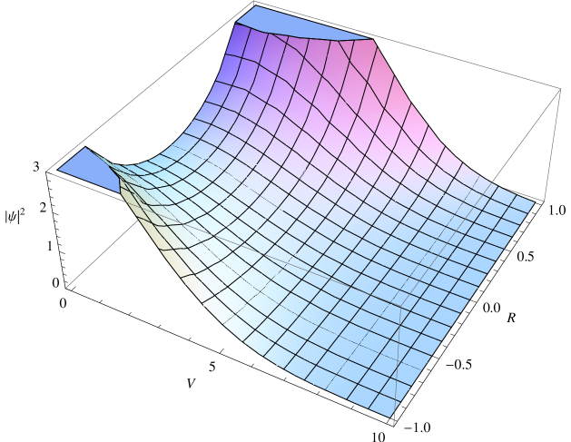
Figure 3: Wave function of Eq. (135) squared, $|\psi(V,R)|^{2}$, plotted as a function of the total volume $V$ and the total curvature $R$, for coupling $g=\sqrt{G}=1$ and $N_{3}=10$. One notes that for strong enough coupling $g$ the distribution in curvatures is fairly flat around $R=0$, giving rise to large fluctuations in the curvature. These become more pronounced as one approaches the critical point at $g_{c}$.

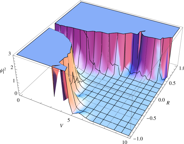
Figure 4: Same wave function of Eq. (135) squared, $|\psi(V,R)|^{2}$, plotted as a function of the total volume $V$ and the total curvature $R$, but now for weaker coupling $g=\sqrt{G}=0.5$, and still $N_{3}=10$. For weak enough coupling $g$ the distribution in curvature is such that values around $R=0$ are almost completely excluded, as these are associated with a very small probability. Note that, unless the total volume $V$ is very small, the probability distribution is markedly larger towards positive curvatures.

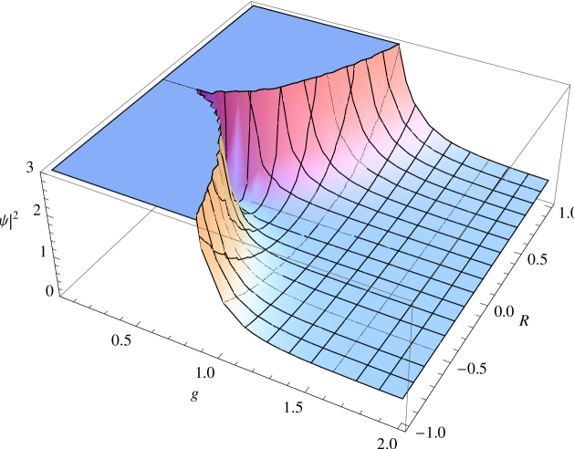
Figure 5: Curvature distribution in $R$ as a function of the coupling $g=\sqrt{G}$. The strong coupling relationship between the average volume and the coupling $g$ [Eq. (64)] allows one to plot the wave function of Eq. (135) squared as a function of the coupling $g$ and the total curvature $R$ only (we use again here $N_{3}=10$ for illustrative purposes). Then, for strong enough coupling $g=\sqrt{G}$, the probability distribution $|\psi|^{2}$ is again fairly flat around $R=0$, giving rise to large fluctuations in the curvature. The latter are interpreted here as signaling the presence of a massless particle. On the other hand, for weak enough coupling $g$ one notices that curvatures close to $R=0$ have essentially vanishing probability. The distribution shown here points therefore toward a pathological ground state for weak enough coupling $g<g_{c}$ [given in Eq. (119)], with no sensible continuum limit.

9 Summary and Conclusions

In this work we have discussed the nature of gravitational wave functions that were found to be solutions of the lattice Wheeler-DeWitt equation for finite simplicial lattices. The main results here were given in Eqs. (124), (128) and (135). While there are many aspects of this problem that still remain open and unexplored, we have nevertheless shown that the very structure of the wave function is such that it allows one to draw a number of useful and perhaps physically relevant conclusions about ground state properties of pure quantum gravity in $3+1$ dimensions. These include the observation that the theory exhibits a phase transition at some critical value of Newton’s constant $G_{c}$ [given in Eq. (119)].

The structure of the wave function further suggests that the weak coupling phase, for which the coupling $G<G_{c}$, is pathological and cannot be interpreted in terms of smooth manifolds at any distance scale. In view of these results it is therefore not entirely surprising that calculations that rely on the weak field, semiclassical or small $G$ expansion run into serious trouble and uncontrollable divergences very early on. Such an expansion does not seem to exist if the non-perturbative lattice results presented here are taken seriously. The correct physical vacuum apparently cannot in any way be obtained as a small perturbation of flat, or near-flat, spacetime. On the other hand the strong coupling phase does not exhibit any such pathology, and is therefore a good candidate for a physically acceptable ground state for pure quantum gravity. It is then a simple consequence of standard renormalization group arguments that in this phase Newton’s constant grows with distance, so that this phase is expected to exhibit gravitational anti-screening. Still, to make the problem tractable, most of the results presented in this work have been obtained in the limit of small curvatures. This is clearly a limitation of the present approach. A more general treatment of the problem, where a variety of curvature squared terms are retained in the expansion of the wave functional, should be feasible by the methods presented here, but is for now clearly beyond the scope of the present work.

Let us mention here that in the Euclidean lattice theory of gravity in four dimensions it was also found early on [20, 21] [see [32] for more recent numerical investigations of 4d lattice gravity, including the determination of the critical point and scaling exponents] that the weak coupling (or gravitational screening) phase is pathological with no sensible continuum limit, corresponding to a degenerate lower dimensional branched polymer. The calculations presented here can be regarded, therefore, as consistent with the conclusions reached earlier from the Euclidean lattice framework. No new surprises have arisen so far when considering the Lorentzian $3+1$ theory, using what can be regarded as an entirely different set of tools.

It seems also worthwhile at this point to compare with other attempts at determining the phase structure of quantum gravity in four dimensions. Besides the Regge lattice approach, there have been other attempts at searching for a non-trivial RG UV fixed point in four dimensions using continuum methods. In one popular field theoretic approach one develops a perturbative diagrammatic $2+\epsilon$ continuum expansion using the background field method to two loop order [36, 37, 38]. This then leads to a non-trivial UV fixed point $G_{c}={\cal O}(\epsilon)$ close to two dimensions. Two phases emerge, one implying again gravitational screening, and the other anti-screening. In the truncated renormalization group calculations for gravity in four dimensions [39, 40], where one retains the cosmological and Einstein-Hilbert terms, and possibly later some higher derivative terms, one also finds evidence for a non-trivial UV fixed point scenario. As in the case of gauge theories, both of these methods are ultimately based on renormalization group flows and the weak field expansion, and are therefore unable to characterize the non-perturbative features of either one of the two ground states. Indeed, within the framework of the weak field expansion inherent in these methods, only the weak coupling phase has a chance to start with. It is nevertheless encouraging that such widely different methods tend to point in the same direction, namely a non-trivial phase structure for gravity in four dimensions.

Let us add here a few more comments, aimed at placing the present work in a wider context. Over the years a number of attempts have been made to obtain results for the gravitational wave functional $\Psi[g]$ in the absence of sources. Often these have relied on the weak field expansion in the continuum, see for example [10, 12]. In $3+1$ dimensions one then finds

$$\Psi[h^{TT}]\;=\;{\cal N}\;\exp\left\{-\textstyle{1\over 4}\displaystyle\int d^{3}{\bf k}\;k\,h^{TT}_{ik}({\bf k})\;h^{TT*}_{ik}({\bf k})\right\}\;,$$ (140)

where $h^{TT}_{ik}({\bf k})$ is the Fourier amplitude of transverse-traceless modes for the linearized gravitational field. It is clear that the above wave functional describes a collection of harmonic oscillator contributions, one for each of the physical modes of the linearized gravitational field. It is not necessary to use Fourier modes, and, as in the case of the electromagnetic field, one can write equivalently the ground state wave functional in terms of first derivatives of the field potentials,

$$\Psi[h^{TT}]\;=\;{\cal N}\;\exp\left\{-{1\over 8\pi^{2}}\int d^{3}{\bf x}\int d^{3}{\bf y}\;{h^{TT}_{ik,l}({\bf x})\;h^{TT*}_{ik,l}({\bf y})\over|{\bf x}\,-\,{\bf y}|^{2}}\right\}\;.$$ (141)

Nevertheless, it is generally understood that the above expressions represent only the leading term in an expansion involving infinitely many terms in the metric fluctuation $h_{ij}$ (in an expansion about flat space, the cosmological constant contribution does not appear). Since Eq. (140) is just the leading term in the weak field expansion, no issue of perturbative renormalizability appears to this order. Nevertheless, higher orders are expected to bring in ultraviolet divergences which cannot be reabsorbed into a simple redefinition of the fundamental couplings $G$ and $\lambda$. Then the results presented in this paper [namely Eqs. (124), (128) and (135)] can be viewed therefore as a first attempt in extending non-perturbatively the result of Eq. (140), beyond the inherent limitations of the weak field limit.

We see a number of additional avenues by which the present work could be extended. One issue, which could be rather laborious to work out in $3+1$ dimensions, is the systematic determination of the relevant lattice wave functionals for the regular triangulations of the sphere to higher order in the weak field expansion, as was done for example in $2+1$ dimensions [2]. It should also be possible to obtain the lattice wave functional numerically in cases where the triangulation itself is not regular, but is described instead by an average coordination number $<\!q\!>$, as described earlier in the text. Another interesting problem would be the derivation of the general form of the lattice wave functional by methods which differ from the Frobenius power series method presented here, such as the $WKB$ approximation [7] or the Raleigh-Schrödinger approach. Finally, it would also be of some interest to re-derive the form of the lattice wave functional for other discrete triangulations, such as the case of the three-torus $T^{3}$ (the Kasner model) [41].

Acknowledgements

The work of H.W.H. was supported in part by the Max Planck Gesellschaft zur Förderung der Wissenschaften, and by the University of California. He wishes to thank prof. Hermann Nicolai and the Max Planck Institut für Gravitationsphysik (Albert-Einstein-Institut) in Potsdam for warm hospitality. The work of R.M.W. was supported in part by the UK Science and Technology Facilities Council. The work of R.T. was supported in part by a DED GAANN Student Fellowship.

References

- [1] H. W. Hamber and R. M. Williams, Phys. Rev. D 84, 104033 (2011).
- [2] H. W. Hamber, R. Toriumi and R. M. Williams, Phys. Rev. D 86, 084010 (2012).
- [3] P. A. M. Dirac, Proc. Roy. Soc. Lond. A 246, 333 (1958); Phys. Rev. 114, 924 (1959).
- [4] R. Arnowitt, S. Deser and C. W. Misner, in Gravitation: An Introduction to Current Research, edited by Louis Witten (Wiley, New York, 1962), p. 227-265; arXiv:gr-qc/0405109.
- [5] J. A. Wheeler, Geometrodynamics and the Issue of the Final State, in Relativity, Groups and Topology, 1963 Les Houches Lectures, edited by B. DeWitt and C. DeWitt (Gordon and Breach, New York, 1964).
- [6] B. S. DeWitt, Dynamical Theory of Groups and Fields, in Relativity, Groups and Topology, 1963 Les Houches Lectures, edited by B. DeWitt and C. DeWitt (Gordon and Breach, New York, 1964).
- [7] B. S. DeWitt, Phys. Rev. 160, 1113 (1967); 162, 1195 (1967); 162, 1239 (1967).
- [8] J. A. Wheeler, in Batelle Rencontres 1967, Lectures in Mathematics and Physics, edited by C. DeWitt and J. A. Wheeler, (Benjamin, New York, 1968), p. 242.
- [9] H. Leutwyler, Phys. Rev. 134, 1155 (1964).
- [10] K. Kuchar̆, J. Math. Phys. 17, 777 (1976).
- [11] J. B. Hartle and S. W. Hawking, Phys. Rev. D 28, 2960 (1983).
- [12] K. Kuchar̆, in the Proceedings of the 4th Canadian Conference on General Relativity and Relativistic Astrophysics, edited by G. Kunstatter, D. Vincent, and J. Williams (World Scientific, Singapore, 1992).
- [13] C. Isham, in Integrable Systems, Quantum Groups and Quantum Field Theories, edited by L. A. Ibort and M. A. Rodriguez (Kluwer, Dordrecht, 1993), p. 157.
- [14] A. O. Barvinsky and C. Kiefer, Nucl. Phys. B 526, 509 (1998).
- [15] T. Regge, Nuovo Cimento, 19 558 (1961).
- [16] M. Roc̆ek and R. M. Williams, Phys. Lett. 104B, 31 (1981); Z. Phys. C21, 371 (1984).
- [17] J. Cheeger, W. Müller and R. Schrader, in Unified Theories of Elementary Particles, Heisenberg Symposium, München 1981, Springer Lecture Notes in Physics, edited by P. Breitlohner and H. P. Dürr (Springer, New York, 1982); Comm. Math. Phys. 92, 405 (1984).
- [18] T. D. Lee, in ‘Discrete Mechanics’, 1983 Erice International School of Subnuclear Physics, vol. 21 (Plenum Press, New York 1985), and references therein.
- [19] C. Itzykson, Fields On A Random Lattice, in Progress in Gauge Field Theory, Proceedings of the NATO Advanced Study Institute, Cargése, France, Sep 1-15, 1983, edited by G. ’t Hooft et al. (Plenum Press, NY, London, 1984) p. 337.
- [20] H. W. Hamber and R. M. Williams, Nucl. Phys. B248, 392 (1984); B260, 747 (1985); 269, 712 (1986); Phys. Lett. B 157, 368 (1985).
- [21] H. W. Hamber, in Critical Phenomena, Random Systems and Gauge Theories, 1984 Les Houches Summer School, Session XLIII, (North Holland, Amsterdam).
- [22] J. B. Hartle, J. Math. Phys. 26, 804 (1985); 27, 287 (1986); 30, 452 (1989).
- [23] H. W. Hamber, Quantum Gravitation, Springer Tracts in Modern Physics, ISBN:9783540852926 (Springer, New York, 2009).
- [24] F. Lund and T. Regge, “Simplicial Approximation to some Homogeneous Cosmologies,“ Princeton preprint, unpublished (1974).
- [25] J. B. Hartle, W. A. Miller and R. M. Williams, Class. Quant. Grav. 14, 2137 (1997).
- [26] Coxeter, H. , 1948, Regular Polytopes, Methuen and Co. Ltd., London.
- [27] Coxeter, H. , 1974, Regular Complex Polytopes, Cambridge University press.
- [28] R. W. Lindquist and J. A. Wheeler, Rev. Mod. Phys. 29 432-443 (1957).
- [29] H. W. Hamber and R. M. Williams, Nucl. Phys. B487 345 (1997).
- [30] H. W. Hamber and R. M. Williams, Phys. Rev. D47, 510 (1993).
- [31] H. W. Hamber and R. M. Williams, Phys. Rev. D 76, 084008 (2007); D 81, 084048 (2010).
- [32] H. W. Hamber, Nucl. Phys. B 400, 347 (1993); Phys. Rev. D 61, 124008 (2000); unpublished (2013).
- [33] Handbook of Mathematical Functions with Formulas, Graphs, and Mathematical Tables, edited by M. Abramowitz and I. A. Stegun (Dover Publications, New York, 1972).
- [34] Digital Library of Mathematical Functions. Release date 2012. National Institute of Standards and Technology, http://dlmf.nist.gov/.
- [35] NIST Handbook of Mathematical Functions, edited by F.W.J. Olver, D. Lozier, R.F. Boisvert, et al., (Cambridge University Press, Cambridge, England, 2010), ISBN 978-0521192255.
- [36] S. Weinberg, Ultraviolet divergences in quantum gravity, in ’General Relativity - An Einstein Centenary Survey’, edited by S. W. Hawking and W. Israel, (Cambridge University Press, 1979).
-
[37]
H. Kawai and M. Ninomiya, Nucl. Phys. B336, 115 (1990);
H. Kawai, Y. Kitazawa and M. Ninomiya, Nucl. Phys. B393, 280 (1993) and B404 684 (1993);
Y. Kitazawa and M. Ninomiya, Phys. Rev. D55, 2076 (1997). - [38] T. Aida and Y. Kitazawa, Nucl. Phys. B491, 427 (1997).
-
[39]
M. Reuter,
Phys. Rev. D 57, 971 (1998);
M. Reuter and H. Weyer, Gen. Relativ. Gravit. 41, 983 (2009), and further references therein. - [40] D. F. Litim, Phys. Rev. Lett. 92 201301 (2004); P. Fischer and D. F. Litim Phys. Lett. B 638, 497 (2006).
- [41] H. W. Hamber, R. Toriumi and R. M. Williams, to be published.