Anomalies in a waterlike model confined between plates

Abstract

Using molecular dynamic simulations we study a waterlike model confined between two fixed hydrophobic plates. The system is tested for density, diffusion and structural anomalous behavior and compared with the bulk results. Within the range of confining distances we had explored we observe that in the pressure-temperature phase diagram the temperature of maximum density (TMD line), the temperature of maximum and minimum diffusion occur at lower temperatures when compared with the bulk values. For distances between the two layers below a certain threshold, $d\leq d_{c}$, only two layers of particles are formed, for $d\geq d_{c}$ three or more layers are formed. In the case of three layers the central layer stays liquid while the contact layers crystallize. This result is in agreement with simulations for atomistic models.

I Introduction

Water has several peculiar thermodynamic and dynamic properties not observed in other liquids. This is the case of the density at room pressure that has a maximum at $4^{o}C$  [1, 2, 3] while in most materials the density increases monotonically with the decrease of the temperature. In addition, between $0.1$ MPa and $190$ MPa water also exhibits an anomalous increase of compressibility [4, 5] and, at atmospheric pressure, an increase of isobaric heat capacity upon cooling [6, 7]. Besides the thermodynamic anomalies water also exhibits an unusual behavior in its mobility. The diffusion coefficient that for normal liquids increases with the decrease of pressure, for water it has a maximum at $4^{o}C$ for $1.5\;atm$ [3, 8]. The presence of the large increase in the response function induced the idea of the existence of two liquid phases and a critical point [9]. This critical point is located at the supercooled region beyond the line of homogeneous nucleation and thus cannot be experimentally measured. In order to circumvent this inconvenience, experiments in confined water were performed [10]. They showed that the large increase of the specific heat it is actually a peak that can be associated with the Widom line, the continuation of the coexistence line beyond a critical point.

The drawback of experiments in nanoscale confinement is that the results obtained do not necessarily lead to conclusions at the bulk level. Notwithstanding this disadvantage the study of confined water by itself is interesting since water is present in ionic channels, proteins, vesicles and other cellular structures under nanoscale confinement. In order to understand the behavior of water under these limitations a number of experiments and simulations of confined water have been performed.

Several types of confinement have been explored: experiments in cylindrical porous [11, 12, 13] and simulations in carbon nanotubes [14, 15], simulations in porous matrices [16, 17, 18, 19], experiments [20, 21] and simulations in rough surfaces [22, 23, 24, 25, 26] and simulations in flat plates [27, 28, 25, 23].

In particular, x-ray and neutron scattering with water in nanopores show that the liquid state persists down to temperature much lower than in bulk [11, 29, 30]. In these experiments in the case of hydrophobic walls the liquid-crystal transition occurs at lower temperatures than in the case of hydrophilic walls [29, 31]. In some scattering experiments there are indications of the formation of cubic ice instead of the hexagonal ice present in the bulk [32, 12]. Several of these experiments show evidences of the presence of layers, one close to the walls and one at the center [11, 29, 30, 12]. For certain type of walls, the central crystallizes before the wall layers [11, 12]. Therefore, the experimental results are not conclusive. They indicate that the crystallization in confined water depends strongly on the size of the porous [13, 33, 30, 34, 11] and on the level of hydration water under surfaces [20, 32].

However, diffraction studies give only indirect information about the existence of crystalline or amorphous states in water, because the Bragg peaks of ice are quite hard to distinguish from liquid states. Moreover, the presence of layers is also only obtained from indirect evidences. In order to circumvent the difficulties of obtaining the structure of water inside the confined system from experiments, a number of simulations have been performed [35, 36, 23]. They employ atomistic models such as SPC/E [37, 35, 36] and TIP5P [23] and coarse-grained models [38, 39] for water.

Simulations indicate that for both hydrophobic [37, 28, 35, 36, 23] and hydrophilic [36, 37, 35] surfaces two or three layers are formed depending on the distance between the confining surfaces. In the case of hydrophobic walls, there is a phase transition between the two to the three layers regime and for a certain temperature and layer separation the central layer stays liquid while the molecules at the walls crystallizes. In addition, in the case of hydrophobic walls the temperature of maximum density and the temperature of maximum and minimum diffusivity move to lower temperatures when compared with the bulk results [28, 23]. At very low pressures, cavitation appears [37]. In the case of the hydrophilic walls, in agreement with the experimentl results, the system remains liquid for temperatures below the temperatures in the bulk case [35].

Thermodynamic anomalies do not occur only in water, experiments for $Te$ [40], $Ga$, $Bi$, $S$ [41, 42] and $Ge_{15}Te_{85}$ [43], liquid metals [44] and graphite [45] and simulations for silica [46, 47, 48], silicon [49] and $BeF_{2}$ [46] shown that these system also have thermodynamic anomalies. In addition, silica [48, 50] and silicon [51] show diffusion anomalous behavior. In principle this systems under confinement could also show a shift in the anomalous properties and layering without having hydrogen bonds. Atomistic and coarse-grained models [52, 39] for water are an interesting tool for understanding water and its properties, however they are not appropriated for seeking for universal mechanisms that would be common for water and the materials cited above in which the hydrogen bonds are not present but still they present the anomalous behavior of water.

Acknowledging that core softened (CS) potentials may engender density and diffusion anomalous behavior, a number of CS potentials were proposed to model the anisotropic systems described above. They possess a repulsive core that exhibits a region of softening where the slope changes dramatically. This region can be a shoulder or a ramp [53, 54, 55, 56, 57, 58, 59, 60, 61, 62, 63, 64, 65, 66, 67, 68, 69, 70, 71, 72, 73, 74, 75, 76, 77, 74]. Despite their simplicity, such models had successfully reproduced the thermodynamic, dynamic, and structural anomalous behavior present in bulk liquid water. They also predict the existence of a second critical point hypothesized by Poole and collaborators [9]. This suggests that some of the unusual properties observed in water can be quite universal and possibly present in other systems.

In this work we study the effect of the confinement in particles interacting through a CS potential. Our core-softened model introduced to study bulk system does not have any directionality and therefore it is not water. However, it does exhibit the density, the diffusion and the response functions anomalies observed in water. This suggests that some of the anomalous properties that are attributed directionality of water can be found in spherical symmetry systems. We explore that also some of the properties of water under confinement such as the presence of layering and the shift to lower temperatures of maximum density and of maximum and minimum of the diffusion coefficient can also be obtained with CS potentials.

The paper is organized as follows: in Sec. II we introduce the model; in Sec. III the methods and simulation details are described; the results are given in Sec. IV; and finally, the conclusions in Sec. V.

II The Model

We study a system of $N$ particles with diameter $\sigma_{p}$ confined between two fixed plates. The surfaces are formed by particles with diameter $\sigma_{w}$ which are organized in a square lattice of area $L^{2}$. The center-to-center plates distance is $d^{*}=d/\sigma_{p}$. A schematic depiction of the system is shown in Fig. 1.

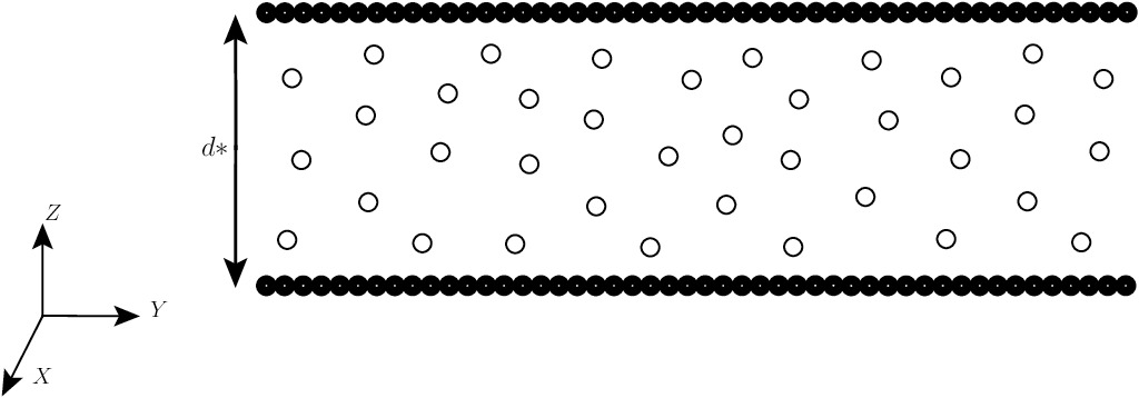
Figure 1: Model system of particles confined between plates.

The particles confined between the two plates interact through an isotropic effective potential given by

$$\centering\frac{U(r)}{\epsilon}=4\left[\left(\frac{\sigma_{p}}{r}\right)^{12}-\left(\frac{\sigma_{p}}{r}\right)^{6}\right]+a\exp\left[-\frac{1}{c^{2}}\left(\frac{r-r_{0}}{\sigma_{p}}\right)^{2}\right]\;\;.\@add@centering$$ (1)

The first term is a standard Lennard-Jones (LJ) $12-6$ potential with $\epsilon$ depth plus a Gaussian centered on radius $r=r_{0}$ and width $c$. We used parameters $a=5$, $r_{0}/\sigma_{p}=0.7$ and $c=1$. The pressure versus temperature phase diagram of this system in the bulk was studied by Oliveira et al. [68, 69]. They found that a system or particles interacting through this potential exhibits a region in the pressure-temperature phase diagram where the density and diffusion coefficient are anomalous.

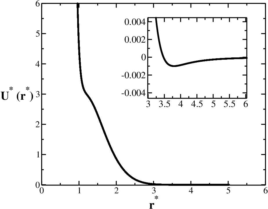
Figure 2: Isotropic effective potential Eq. (1) of interaction between the waterlike particles. The potential and the distances are in dimensionless units, $U^{*}=U/\epsilon$ and $r^{*}=r/\sigma_{p}$ and the parameters are $a=5$, $r_{0}/\sigma_{p}=0.7$ and $c=1$. The inset shows a zoom in the very small atractive part of the potential.

This potential has two length scales with a repulsive shoulder at $r/\sigma_{p}\approx 1$ and a very small attractive well at $r/\sigma_{p}\approx 3.8$ (Fig. 1). Depending of the choice of the parameters $a,b,c$ and $\sigma_{p}$, it can represent a whole family of intermolecular interactions. In this paper we employ $a=5$, $r_{0}/\sigma_{p}=0.7$ and $c=1$.

The particle-plate interaction is given by Weeks-Chandler-Andersen Lennard-Jones potential, namely [78, 79],

$$U=\left\{\begin{array}[]{ll}U_{{\rm{LJ}}}(r)-U_{{\rm{LJ}}}(r_{cw}),\qquad r\leq r_{cw}\\ 0,\qquad r>r_{cw}\;,\end{array}\right.$$ (2)

where $U_{LJ}(r)$ is a standard 12-6 LJ potential. The cutoff distance is $r_{cw}=2^{1/6}\sigma_{wp}$, where $\sigma_{wp}=(\sigma_{p}+\sigma_{w})/2$ is the Lorentz-Berthelot mixing rule [80] used when two kinds of particles are interacting between them. In our model, $\sigma_{p}=\sigma_{w}=\sigma_{wp}$.

III The Methods and Simulation Details

The system has $507$ particles confined between the plates with area $L^{2}$ and distant $d$, resulting in a number density $\rho=N/(dL^{2})$. The plates are located at $z=0$ and $z=d$, whereas in $x$ and $y$ directions periodic boundary conditions are used. The repulsive interactions with the plates underestimates the number density, so we need to calculate the effective density using the effective distance $d_{e}$ perpendicular to the plates. The new density will be $\rho=N/(d_{e}L^{2})$, where $d_{e}\approx d-(\sigma_{p}+\sigma_{w})/2$ is an approach for the effective distance between the plates [23].

Molecular dynamics simulations at the NVT-constant ensemble and the Nose-Hoover [81, 82] thermostat were used in order to keep fixed the temperature, with coupling parameter $Q=2$. The interaction potential between particles has a cutoff of $r_{c}=3.5$ and this potential was shifted in order to have $U=0$ at $r_{c}$.

Several densities and temperatures are done for the following distances $d^{*}=d/\sigma_{p}$ between the plates: 4.2, 4.8, 5.5, 6.0 and 6.3. The initial configuration of the systems were set on solid structure and the equilibrium states reached after $2\times 10^{6}$ steps, followed by $4\times 10^{6}$ simulation run. The time step was $0.002$ in reduced units and the average of the physical quantities were get with $50$ descorrelated samples. The thermodynamic stability of the system was checked by analyzing the dependence of parallel and perpendicular pressure on density namely and by the behavior of the energy after the equilibrium states.

The thermodynamics averages in parallel and perpendicular directions to the plates are done employing different procedures [83]. Parallel pressure, $P_{\parallel}$, is computed using the virial expression for the $x$ and $y$ directions [23, 28, 27, 84], while the perpendicular pressure, $P_{\perp}$, is calculated using two distinct methods. For systems with a strong confinement, such as $d^{*}=4.2$ and $4.8$, the total force perpendicular to the plates is used [27, 85],

$$P_{\perp}=\frac{F_{plates}}{A}=\frac{\left|\sum_{i=1}^{N}{\bf{F}}_{i,plates}\right|}{L^{2}}\;.$$ (3)

For the others systems with larger distances, such as $d^{*}=5.5$, $6.0$ and $6.3$, the pressure $P_{\perp}$ is computed through the virial expression in $z$ direction [86].

The dynamic of the systems was studied by lateral diffusion coefficient, $D_{\parallel}$, related with the mean square displacement (MSD) from Einstein relation,

$$D_{\parallel}=\lim_{\tau\to\infty}\frac{\langle\Delta r_{\parallel}(\tau)^{2}\rangle}{4\tau},$$ (4)

where $r_{\parallel}=(x^{2}+y^{2})^{1/2}$ is the distance between the particles parallel to the plates.

We also studied the structure of the systems by lateral radial distribution function, $g_{\parallel}(r_{\parallel})$, and translational order parameter, $t$. We calculate the $g_{\parallel}(r_{\parallel})$ in specific regions between the plates, and the same for parameter $t$. An usual definition for $g_{\parallel}(r_{\parallel})$ is

$$g_{\parallel}(r_{\parallel})\equiv\frac{1}{\rho^{2}V}\sum_{i\neq j}\delta(r-r_{ij})\left[\theta\left(\left|z_{i}-z_{j}\right|\right)-\theta\left(\left|z_{i}-z_{j}\right|-\delta z\right)\right].$$ (5)

The $\theta(x)$ is the Heaviside function and it restricts the sum of particle pairs in the same slab of thickness $\delta z=1$. We need to compute the number of particles for each region and the normalization volume will be cylindrical. The $g_{\parallel}(r_{\parallel})$ is proportional to the probability of finding a particle at a distance $r_{\parallel}$ from a referent particle.

The translational order parameter is defined as [48, 87, 88]

$$t\equiv\int^{\xi_{c}}_{0}\mid g_{\parallel}(\xi)-1\mid d\xi$$ (6)

where $\xi=r_{\parallel}\rho_{s}^{1/2}$ is the interparticle distance in the direction parallel to the plates scaled by $\rho_{s}^{1/2}=(N_{layer}/L^{2})^{1/2}$. $N_{layer}$ is the average of particles for each slab supposing that this number not change significantly (well-defined layers) [86]. We use $\xi_{c}=\rho_{s}^{1/2}L/2$ as cutoff distance.

When the system is an ideal gas, with $g_{\parallel}(r_{\parallel})=1$, we obtain $t=0$, because the system is not structured. But, as the system becomes more structured, like a crystal phase, the $g_{\parallel}(r_{\parallel})\neq 1$, so parameter $t$ assumes large values.

All physical quantities are shown in reduced units [80] as

$$d^{*} = \frac{d}{\sigma_{p}}$$

$$\tau^{*} = \frac{(\varepsilon/m)^{1/2}}{\sigma_{p}}\tau$$

$$T^{*} = \frac{k_{B}}{\varepsilon}T$$

$$P_{\parallel,\perp}^{*} = \frac{\sigma_{p}^{3}}{\varepsilon}P_{\parallel,\perp}$$

$$\rho^{*} = \sigma_{p}^{3}\rho$$

$$D_{\parallel}^{*} = \frac{(m/\varepsilon)^{1/2}}{\sigma_{p}}D_{\parallel}\;\;.$$ (7)

IV Results

Systems With Three Layers

The first set of systems that we study corresponds to plates separated by the distances $d^{*}=5.5$, $6.0$ and $6.3$. In all these cases, the particles are structured in three layers in $z$ direction divided in two contact layers, near to the plates, and one middle layer, located in the center of the plates. The formation of layering structures in confined water was also observed in atomistic models [28, 23]. The layering density can be seen in Fig. 3 that illustrates the $d^{*}=6.3$ case: (a) the snapshot of the system with $T^{*}=0.220$ and $\rho^{*}=0.141$, (b) the transversal density profile for $T^{*}=0.220$ and various densities and c) the transversal density profile for $\rho^{*}=0.141$ and different temperatures. The layers become more defined at low temperatures and high densities. Now we need to identify if the different layers are in the solid or in the liquid state. In order to answer to this question the structure is analyzed.

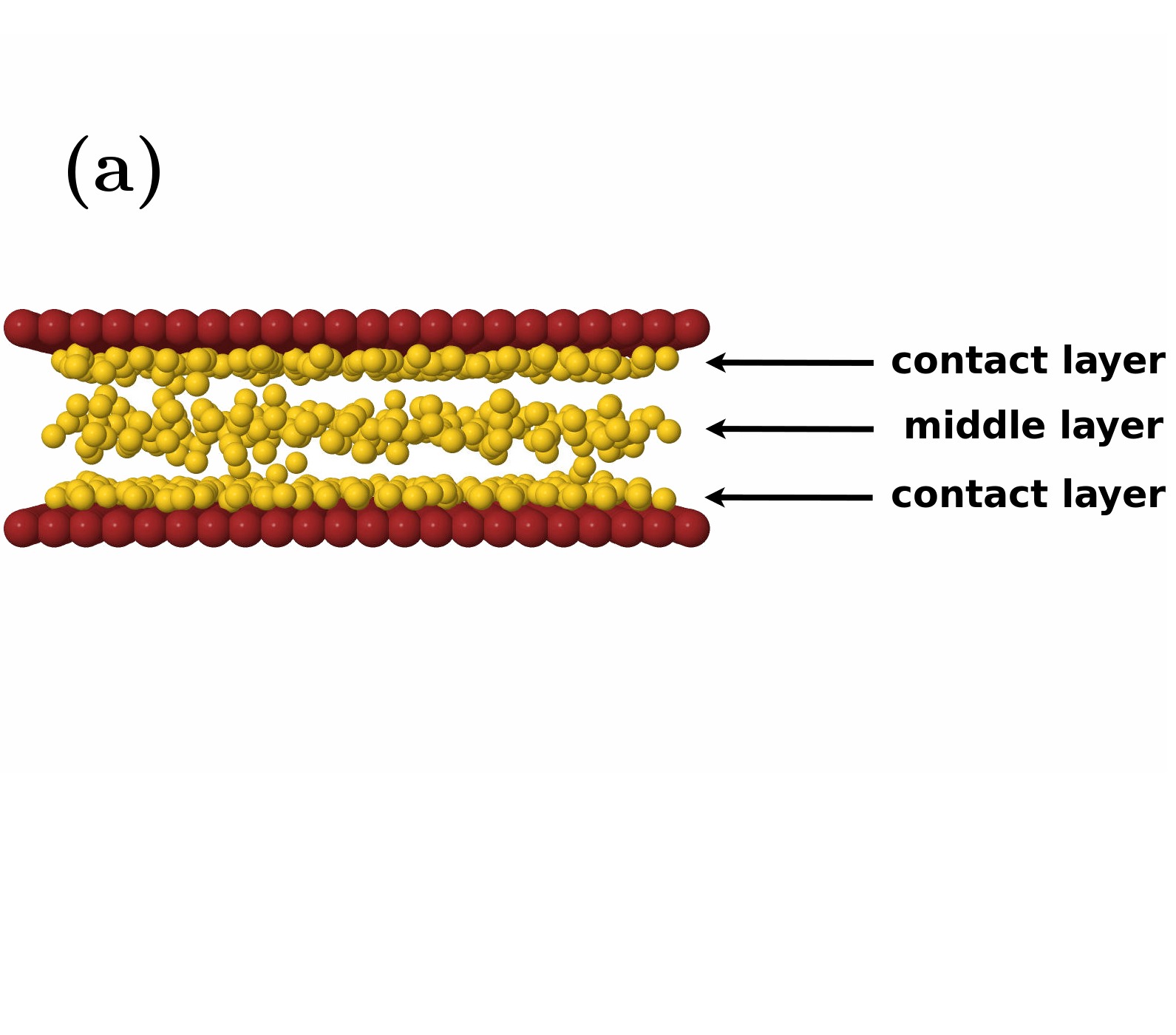
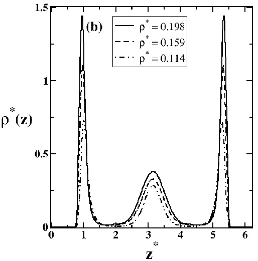
Figure 3: In (a), we have a snapshot of the system with $T^{*}=0.220$ and $\rho^{*}=0.141$ after the equilibrium state. Furthermore, the transversal density profile is shown for (b) $T^{*}=0.220$ and different densities, and for (c) $\rho^{*}=0.141$ and different temperatures. We can see the formation of two contact layers, near to the plates, and one middle layer. This system corresponds to $d^{*}=6.3$, whereas the cases like $d^{*}=5.5$ and $6.0$ present the same behavior in relation to layering density.

The Fig. 4 shows the radial distribution function for $d^{*}=6.3$ in two cases: (a) $\rho^{*}=0.181$ and $T^{*}=0.220$ and (b) $\rho^{*}=0.217$ and $T^{*}=0.140$. For the case (a) the radial distribution of the central layer and of the contact layer are liquid-like. The contact layer shows a distribution compatible with a very structured liquid. For the case (b), the central layer is also liquid-like, however the contact layer is solid-like. The liquid-solid transition occurs at different temperatures and densities for the confinement $d^{*}=5.5,6.0$ and $d^{*}=6.3$ that do exhibit three layers analyzed here. This result is in agreement with observations for SPC/E water [28].

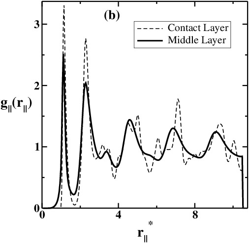
Figure 4: Radial distribution function for $\rho^{*}=0.181$ and $T^{*}=0.220$ in (a), and $\rho^{*}=0.217$ and $T^{*}=0.140$ in (b). Bold lines represent the $g_{||}(r_{||})$ for the middle layer and the dashed lines represent the $g_{||}(r_{||})$ for the contact layer.

In the case of the bulk [69] the potential exhibit an anomalous behavior in the translational order parameter $t^{*}$. For normal systems the $t^{*}$ grows with the density, however for our CS potential it has a region where it does decreases with the increase of the density. Here, we test if this anomalous behavior is also observed in the central and contact layers.

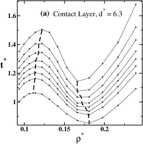
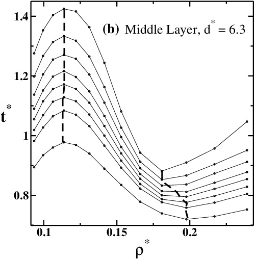
Figure 5: Translational order parameter versus density for $d^{*}=6.3$ for (a) contact layer and the (b) middle layer, separately. The solid lines represent the isotherms $T^{*}=0.170$, $0.190$, $0.205$, $0.220$, $0.232$, $0.245$, $0.260$ and $0.300$ from the top to the bottom. The dashed lines connect the extremes.

The Fig. 5 (a) and (b) show the translational order parameter defined by Eq. 6 as function of density for differents temperatures $T^{*}=0.170,0.190,0.205,0.220,0.232,0.245,0.260$ and $0.300$, at $d^{*}=6.3$, for the contact layer and for the middle layer, respectively. The dots represent the simulation data and the solid lines identify the isotherms. The dashed lines, $\rho^{*}_{t-max}<\rho^{*}<\rho^{*}_{t-min}$, identifies the region in which $t^{*}$ is anomalous, namely it decreases with the increase of the density. The region in the pressure-temperature phase diagram in which $t^{*}$ computed under confinement occurs at lower temperatures when compared with the bulk values [69].

The translational order parameter for the contact layer for very low temperatures and very high densities is larger than the value for the middle layer what suggests that becomes very large the indicating the crystallization the particles at the wall are more structured than in the center. For the confinement with $d^{*}=5.5$ and $6.0$, a similar behavior for $t^{*}$ is observed. The structural differences between the layers present in our model were also observed in water but also in colloidal suspension, for several kinds of particle-plates interactions [89, 90, 23, 91, 92] and for confined SPC/E water by hydrophobic wall [28].

Another propertie that exhibits anomalies in the bulk is the diffusion coefficient. In normal liquids, the diffusion at constant temperature grows with decreasing density, but in waterlike liquids there is a region ($\rho^{*}_{D_{\parallel}-min}<\rho^{*}<\rho^{*}_{D_{\parallel}-max}$) where the diffusion decreases with decreasing density, so this is an anomalous behavior. In our system, this anomaly can be observed in the bulk [68]. How the confinement affects the region in the pressure-temperature phase diagram where the diffusion is anomalous? In order to answer this question the lateral diffusion coefficient was computed as function of density as shown in Fig. 6 for (a) $d^{*}=5.5$, (b) $d^{*}=6.0$ and (c) $d^{*}=6.3$. In these cases, the diffusion coefficient has a region in which it grows with density representing the density anomalous region. The temperature of maximum and minimum diffusion coefficient are lower in the confined system than in the bulk case [69]. Our finding are in agreement with the observations of the diffusion coefficient in coarse-grained model confined between smooth hydrophobic plates, separated at $0.5$nm [38] and atomistic models [23].

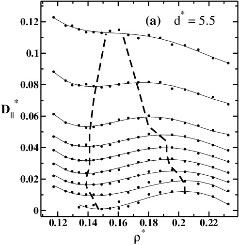
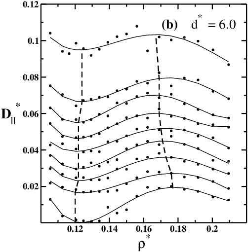
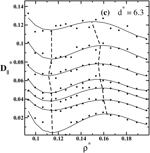
Figure 6: Lateral diffusion coefficient as function of density for (a) $d^{*}=5.5$ and isotherms $T^{*}=0.140$, $0.160$, $0.175$, $0.190$, $0.205$, $0.220$, $0.240$, $0.275$ and $0.320$, (b) $d^{*}=6.0$ and isotherms $T^{*}=0.140$, $0.160$, $0.175$, $0.190$, $0.205$, $0.220$, $0.235$, $0.250$ and $0.290$ and (c) $d^{*}=6.3$ and isotherms $T^{*}=0.140$, $0.170$, $0.190$, $0.205$, $0.232$, $0.260$ and $0.300$, from the bottom to the top. The dots represent the simulation data and the solid line is just a polinomial fit to isotherms. The dashed lines connect the extremes of diffusion.

In the bulk, our potential exhibits a density anomalous region in the pressure-temperature phase diagram. How confining affects the TMD line? In order to answer to this question the TMD is computed under confinement. The density anomaly is given by $(\partial\rho/\partial T)_{P_{\parallel}}=0$, so using the following Maxwell relation

$$\left(\frac{\partial V}{\partial T}\right)_{P_{\parallel}}=-\left(\frac{\partial P_{\parallel}}{\partial T}\right)_{V}\left(\frac{\partial V}{\partial P_{\parallel}}\right)_{T},$$ (8)

density anomaly can be found through $(\partial P_{\parallel}/\partial T)_{\rho}=0$, what is equivalent to the minimum of the parallel pressure versus temperature.

Fig. 7 illustrates the parallel pressure versus temperature phase diagram for the (a) $d^{*}=5.5$, (b) $d^{*}=6.0$ and (c) $d^{*}=6.3$ cases. The thin solid lines are the isochores, the solid bold lines represent the TMD, the dashed lines are the lateral diffusion extremes, the dashed-dotted lines are the translational order parameter extremes for a contact layer and the dotted lines are the translational order parameter extremes for the middle layer.

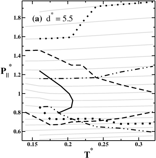
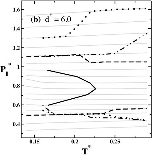
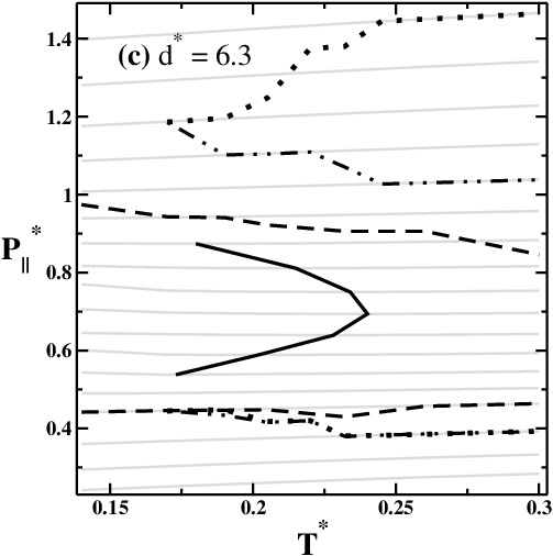
Figure 7: Phase diagrams $P_{\parallel}^{*}-T^{*}$ for (a) $d^{*}=5.5$, (b) $d^{*}=6.0$ and (c) $d^{*}=6.3$. The thin solid lines are the isochores (a) $0.117\leq\rho^{*}\leq 0.233$, (b) $0.105\leq\rho^{*}\leq 0.209$ and (c) $0.099\leq\rho^{*}\leq 0.253$. The solid bold line represents the TMD, the dashed line are the lateral diffusion extremes, the dashed-dotted line are the translational order parameter extremes for a contact layer and the dotted line are the translational order parameter extremes for the middle layer.

A comparison between the TMD of the confined and the bulk systems is given by Fig. 8 (a). The densities and pressures ranges of the TMD’s locations are also shown in Table 1. The TMD lines of confined systems are shifted to lower temperatures and higher densities when compared with the bulk.

For $d^{*}=5.5$ and $6.0$, the TMD lines are shifted to higher pressures, whereas for $d^{*}=6.3$ this shifting occurs to slightly lower pressures when compared with the bulk TMD. The non monotonic shift in pressure when compared with the bulk results can be attibuted to the fact that we employ the lateral pressure for the confined system while we use the total pressure for the bulk system.

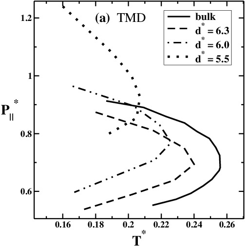
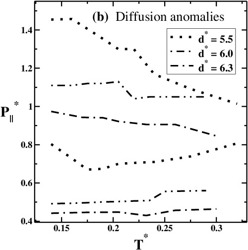
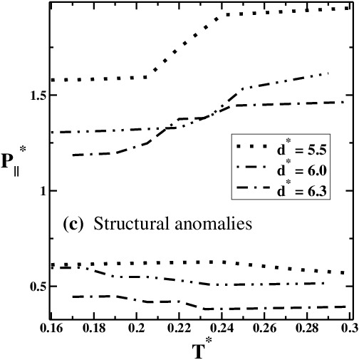
Figure 8: Phase diagram $P_{\parallel}^{*}-T^{*}$ comparing in (a) the shifting of the TMD lines for the confined systems in relation to the bulk. A comparison between the anomalies of the confined systems is given in (b) for diffusion and in (c) for translational order parameter of the middle layer. For (b) and (c), the solid bold lines represent the system with $d^{*}=5.5$, the dashed-dotted lines represent $d^{*}=6.0$ and the thin dotted lines represent $d^{*}=6.3$.

Kumar et al. [23] found that the TMD line for confined systems is shifted to lower temperatures but in the same range of pressures when compared with the bulk system . For TIP4P water model in contact with six hydrophobic spheres, Gallo and Rovere [16] found that TMD line in confined systems is shifted to lower temperatures and higher pressures. Furthermore, they observed that the spinodal curve follow the shifting of the TMD line. Similar result is observed in our systems. Xu and Molinero [93], using a coarse-grained model for water (mW, Monatomic Water Model) [94], confined in nanopores of diameter $1.5$nm, also found a TMD shifted to lower temperatures and higher pressures. So, the density anomalies observed in our systems have a good agreement with other atomistic and coarse-grained simulations.

Table 1: Densities and pressures ranges of TMD’s location of confined and bulk systems.

$d^{*}$	density range	pressure range
$5.5$	$0.149<\rho^{*}<0.188$	$0.800<P_{\parallel}^{*}<1.237$
$6.0$	$0.129<\rho^{*}<0.162$	$0.599<P_{\parallel}^{*}<0.965$
$6.3$	$0.122<\rho^{*}<0.153$	$0.541<P_{\parallel}^{*}<0.875$
bulk	$0.110<\rho^{*}<0.140$	$0.552<P^{*}<0.913$

The perpendicular pressure is shown in Fig. 9 as funtion of (a) temperature and (b) density, at $d^{*}=6.3$. A monotonic increasing behavior is observed in both cases. The ranges of densities and temperatures are the same done in $P_{\parallel}^{*}-T^{*}$ phase diagram. The other systems ($d^{*}=5.5$ and $6.0$) have a similar behavior and they are not shown here for simplicity. The same behavior for perpendicular pressure also was observed by Kumar et al. [23].

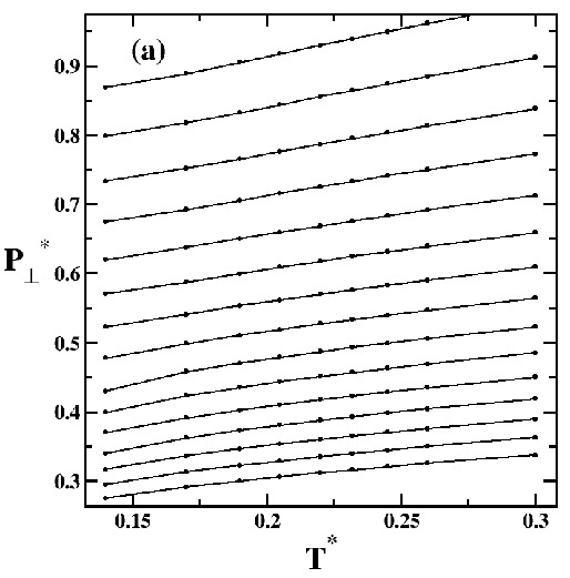
Figure 9: Phase diagrams (a) $P_{\perp}^{*}-T^{*}$ and (b) $P_{\perp}^{*}-\rho^{*}$ at $d^{*}=6.3$. The dots are the simulation data and the solid line just connect the isochores in (a) and the isotherms in (b). The ranges of densities and temperatures are the same done in $P_{\parallel}^{*}-T^{*}$ phase diagram.

System With Two Layers

The confinement by very narrow distances induces the transition from three to two layers. In this subsection, we study a system with plates separated by $d^{*}=4.2$. A snapshot in Fig. 10 (a) shows the two contact layers, without middle layer. Figs. 10 (b) illustrate the behavior of the transversal density profile for fixed temperature, $T^{*}=0.220$, but for different total densities. Figs. 10 (b) also shows the density profile but for fixed total density, $\rho^{*}=0.155$, and several temperatures. The structuration in just two contact layers is due the strong effect of confinement. Structure of bilayer is observed for hydrophobic confinement in TIP5P [95, 96, 97], TIP4P [98] and mW [99] models of water.

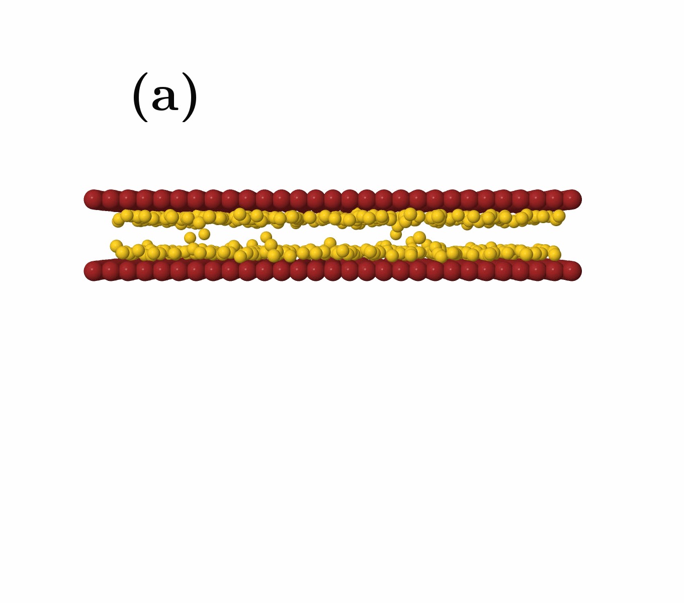
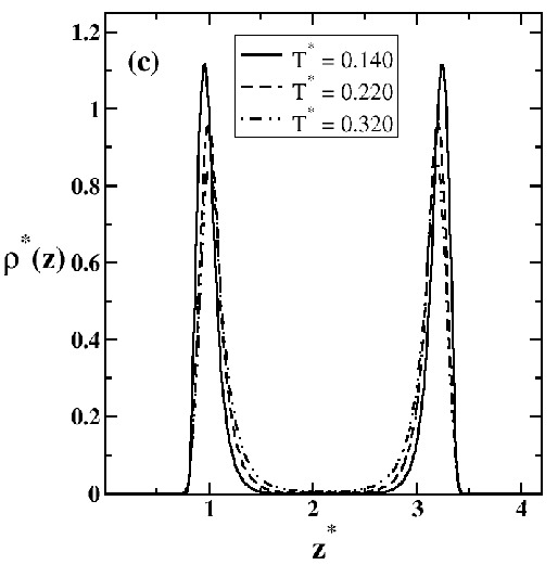
Figure 10: (a) Snapshot of the system after the equilibrium state. In (b) we can see the tranversal density profile for $T^{*}=0.220$ and several densities, and in (c) for $\rho^{*}=0.155$ and several temperatures.

Fig. 11 (a) shows the parallel pressure versus temperature phase diagram. The isochores are represented by thin lines, and the TMD by the solid bold line. It also shows the diffusion extrema (dashed line) and the translational order parameter extrema (dashed-dotted line). The comparison between the TMD line for the $d^{*}=4.2$ case and the TMD for the bulk system is illustrated in Fig. 11 (b). The location of the TMD is $0.604<P_{\parallel}^{*}<0.959$ and $0.137<\rho^{*}<0.170$. Similarly to what happens in the three layer system, the TMD line shifts to lower temperatures when compared with the bulk. This characteristic is evidenced in Fig. 11 (c).

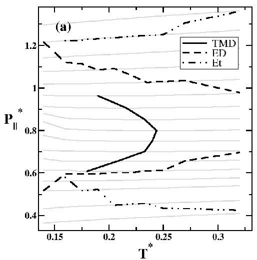
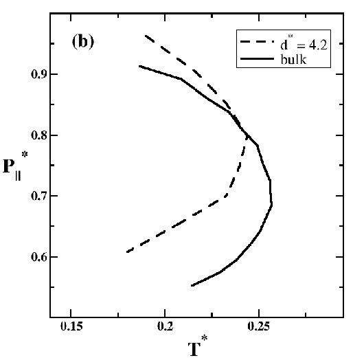
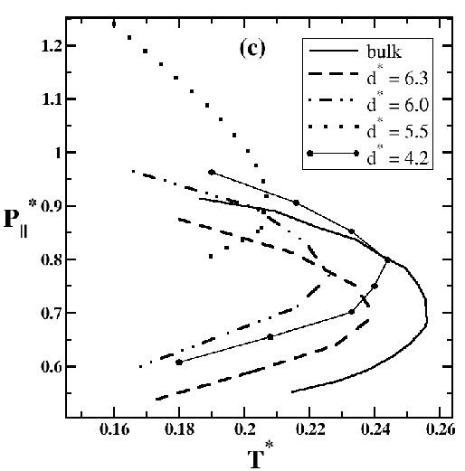
Figure 11: Phase diagrams $P_{\parallel}^{*}-T^{*}$ showing the density, dynamic and structural anomalies in (a). In (b) we have a comparison between the TMD lines of $d^{*}=4.2$ and the bulk system, and in (c) the same comparison is done with TMD lines for systems that present formation of three layers.

Fig. 12 (a) illustrates the perpendicular pressure versus temperature phase diagram for various isochores that show no TMD line. No anomalous behavior is observed similarly to what happens in the three layers regime. Fig. 12 also shows the radial distribution function (in (b)) and the mean square displacement (in (c)) for the lateral direction. For $\rho^{*}=0.137$, these figures show a amorphous solid-like behavior for $T^{*}=0.160$ and a liquid-like behavior for $T^{*}=0.270$. A solid-to-liquid transition was also observed for the TIP5P model [96, 97], for the TIP4P model [98] and for the mW model [99].

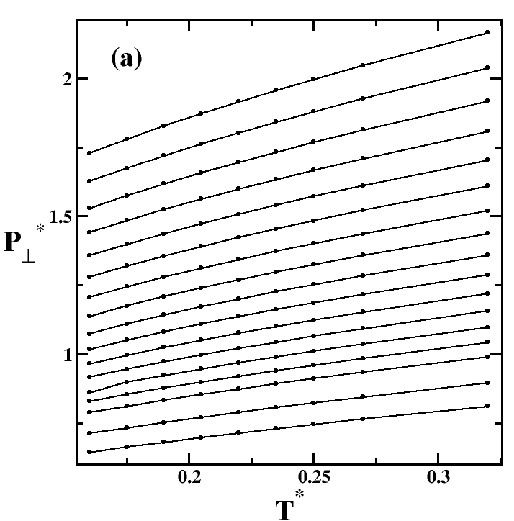
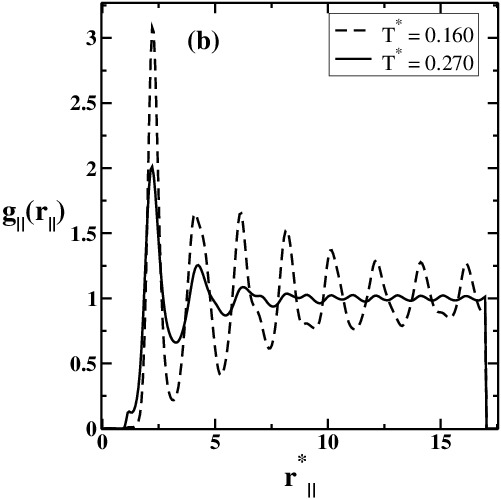
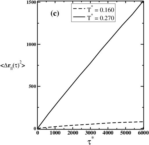
Figure 12: In (a), the monotonic increasing behavior is observed for perpendicular pressure with the temperature. In (b), we have a $g_{\parallel}(r_{\parallel})$ for a amorphous solidlike state, with $T^{*}=0.160$, and a liquidlike state, with $T^{*}=0.270$, both at $\rho^{*}=0.137$. The MSD is observed for these cases in (c).

An anomalous region for translational order parameter and for lateral diffusion are also observed in this extremely confined system as can be seen in Figs. 13 (a) and (b), respectively. The dashed lines connect the extremes of these anomalies, defining the anomalous region that we can see in $P_{\parallel}^{*}-T^{*}$ phase diagram in Fig. 11 (a).

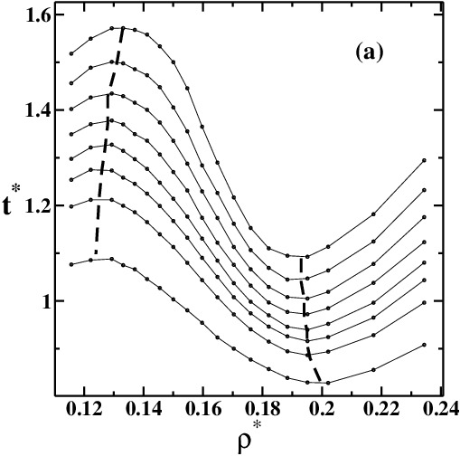
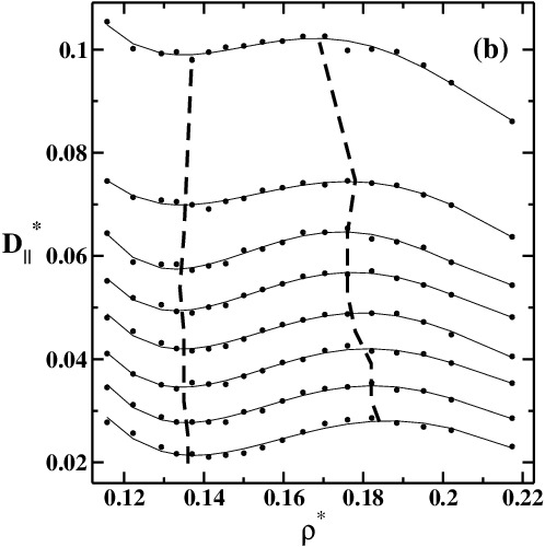
Figure 13: In (a), the translational order parameter as function of density, and in (b) the lateral diffusion coefficient as function of density. The isotherms are connecting the simulation data (points) and they are from the top to the bottom $T^{*}=0.175$, $0.190$, $0.205$, $0.220$, $0.235$, $0.250$, $0.270$ and $0.320$ for $t^{*}$ (a) and from the bottom to the top for $D^{*}_{\parallel}$ (b). The dashed lines connect the extremes observed in both cases.

Three-to-Two layers System

The system with $d^{*}=4.8$ exhibits an unusual behavior that resembles properties of both two layers and the three layers systems. In Fig. 14 (a) the lateral diffusion as function of density is illustrated. The diffusion anomaly is only present at very low temperatures, $T^{*}\leq 0.150$. In addition, as shown in the Fig. 14 (b) the TMD line is also restricted to low temperatures. In Fig. 14 (c) the comparison between the TMD line of the confined system with $d^{*}=4.8$ and the TMD of bulk confirms this shift of the TMD to very low $T^{*}$, much lower than the shift observed for confinement with $4.8<d^{*}$ and $4.8>d^{*}$ discussed above.

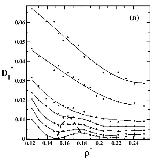
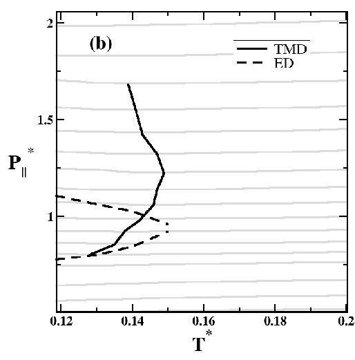
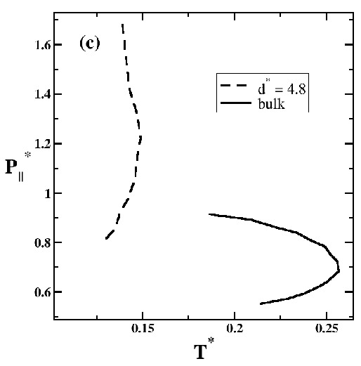
Figure 14: In (a), the lateral diffusion coefficient as function of density for isotherms from the bottom to the top $T^{*}=0.118$, $0.130$, $0.140$, $0.150$, $0.160$, $0.190$ and $0.220$. Diffusion extremes are connected by dashed lines. In (b), we have the phase diagram showing the TMD line and the diffusion extremes. A comparison between the TMD line of this system with bulk is given in (c).

This $d^{*}=4.8$ case is not only peculiar for exhibiting a very low temperature of maximum density but also for presenting anomalous behavior at the perpendicular pressure versus temperature phase diagram. In Fig. 15 (a) the isochores at the perpendicular pressure versus temperature phase diagram exhibits minima not shown for $4.8>d^{*}>4.8$. In order to shade some light in the reason for the unusual behavior of the system for $d^{*}=4.8$ we explore the behavior of the structure and of the stability of the layers. Fig. 15 (b) shows the lateral pressure versus density of fixed temperatures. For $T^{*}<0.190$, the slope of the curve first increases and then decreases. This change even thougth not indicating a phase transition is usually observed before the phase separation would be stablished [35].

The Fig. 15 (c) shows the tranversal density profile for $\rho^{*}=0.139$ and for a number of temperatures. At this density, three layers are present for low temperatures, $T^{*}=0.118$ and $0.150$. At high temperatures, $T^{*}=0.250$, two layers are well defined with particles equally distributed between them without forming a third layer.

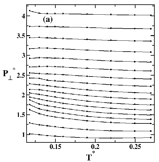
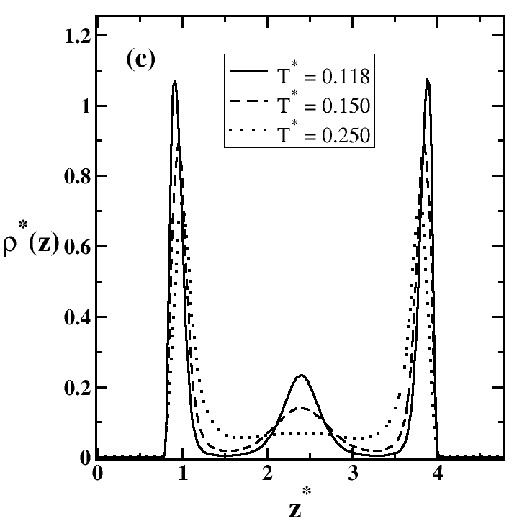
Figure 15: The perpendicular pressure versus temperature is given in (a) and versus density is given in (b). The simulation data (dots) are connected by solid lines for better visualization. The transversal density profile for $\rho^{*}=0.139$ and some temperatures is shown in (c).

In order to understand the two-to-three layers transition, the change in the structure of the central layer with temperature and density is checked. The structure of the middle layer is shown in the Fig. 16 for different temperatures and densities. At low temperatures (cases (a) at $T^{*}=0.118$ and (b) at $T^{*}=0.160$) and high densities, $\rho^{*}>0.170$, the central layer is divided in many sublayers. By decreasing the density the many layers give rise at $\rho^{*}=0.170$ to a central layer that disappears as the density is decreased any further. At high temperatures, $T^{*}>0.160$ (case (c) shown at $T^{*}=0.220$), as the density decreases the system passes from three-to-two layers without forming the sublayers. At low temperatures, due to the presence of the many sublayers the density anomalous region appears. The TMD originates from particles moving from one scale to the other [69].

Figure 16: Tranversal density profile for the middle layer at many densities and (a) $T^{*}=0.118$, (b) $T^{*}=0.160$ and (c) $T^{*}=0.220$. The dashed lines represent states for $\rho^{*}<0.170$, the solid lines for $\rho^{*}>0.170$ and the bold circles are for $\rho^{*}=0.170$.

Our interpretation is in accordance with the assumption of Kumar et al. [23], that the split of the middle layer in sublayers is justified by the density anomaly. Using SPC/E model for water and hydrophobic rough plates, Giovambattista et al. [28] found a phase transition between a bilayer ice and a trilayer heterogeneous fluid for different distances between the plates. For smooth plates separated at $0.8$nm and SPC/E model, Lombardo et al. [36] also found a phase transition between two and three layers.

Changes in diffusion coefficient as function of separation between the plates are reported in systems with transitions between 6 and 5, 5 and 4, 4 and 3 layers [100], suggesting that the dynamic behavior change in systems with structural transitions. So, the dynamic behavior of our system at $d^{*}=4.8$ is another possible explanation for the peculiar behavior on its anomalies.

V Conclusions

In this paper, the effects of confining a system of particles interacting through core-softened is explored.

The formation of three layers, two close to the walls and one central is observed for large values of $d^{*}$, while two layers are observed for small values of $d^{*}$. In addition the region in the pressure-temperature phase diagram where the density anomaly appears moves to lower temperatures. These results are similar to the results obtained in atomistic and coarse-grained models where unlike our model the directionality of the h-bonds is explicitly included [23, 101].

Our results indicate that layers are formed in order to minimize the particle-particle interaction potential and the wall-particle interaction. Therefore, if the walls are distance $d^{*}=5.0$ it is possible to fit three layers in which each will is distant $2.0$ from the other and the contact layer is distant $1.0$ from the wall. For $d^{*}=4.0$ it is only possible to fit two layers distant $2.0$ from each other and $1.0$ from the wall. The density, diffusion and structural anomalous behavior that implies particles moving from one length scales to the other (moving from the length scale at $\approx 3.0$ to the length scales at $1.0$) occurs only along the parallel plane, therefore the anomalies appear as function of $P_{\parallel}$.

The case $d^{*}=4.8$ is the boundary between the two layer and the three layer cases. This case allow us to observe how the presence of the density anomaly is related with moving from different particle-particle distances.

Our results suggest that effective spherical symmetric two length scales potentials are an interesting tool for understanding the mechanisms that arise from confining systems with density, diffusion and structural anomalies. Due to their simplicity the results obtained can be generalized to other experimental realizations besides water.

References

- [1] R. Waler. Essays of natural experiments. Johnson Reprint, New York, 1964.
- [2] G. S. Kell. J. Chem. Eng. Data, 20:97, 1975.
- [3] C. A. Angell, E. D. Finch, L. A. Woolf, and P. Bach. J. Chem. Phys., 65:3063, 1976.
- [4] R. J. Speedy and C. A. Angell. J. Chem. Phys., 65:851, 1976.
- [5] H. Kanno and C. A. Angell. J. Chem. Phys., 70:4008, 1979.
- [6] C. A. Angell, M. Oguni, and W. J. Sichina. J. Phys. Chem., 86:998, 1982.
- [7] E. Tombari, C. Ferrari, and G. Salvetti. Chem. Phys. Lett., 300:749, 1999.
- [8] F. X. Prielmeier, E. W. Lang, R. J. Speedy, and H.-D. Lüdemann. Phys. Rev. Lett., 59:1128, 1987.
- [9] P. H. Poole, F. Sciortino, U. Essmann, and H. E. Stanley. Nature (London), 360:324, 1992.
- [10] L. Liu, S.-H. Chen, A. Faraone, S.-W. Yen, and C.-Y. Mou. Phys. Rev. Lett., 95:117802, 2005.
- [11] M. Erko, G. H. Findenegg, N. Cade, A. G. Michette, and O. Paris. Phys. Rev. B, 84:104205, 2011.
- [12] K. Morishige and K. Nobuoka. J. Chem. Phys., 107:6965, 1997.
- [13] K. Morishige and K. Kawano. J. Chem. Phys., 110:4867, 1999.
- [14] K. Koga, G. T. Gao, H. Tanaka, and X. C. Zeng. Nature (London), 412:802, 2001.
- [15] G. Hummer, J. C. Rasaiah, and J. P. Noworyta. Nature (London), 414:188, 2001.
- [16] P. Gallo and M. Rovere. Phys. Rev. E, 76:061202, 2007.
- [17] E. G. Strekalova, J. Luo, H. E. Stanley, G Franzese, and S. V. Buldyrev. Phys. Rev. Lett., 109:105701, 2012.
- [18] P. A. Bonnaud, B. Coasne, and R. J.-M. Pellenq. J. Phys.: Condens. Matter, 22:284110, 2010.
- [19] O. Pizio, H. Dominguez, L. Pusztai, and S. Sokolowski. Physica A, 388:2278, 2009.
- [20] M. Bellissent-Funel, R. SridiDorbez, and L. Bosio. J. Chem. Phys., 104:10023, 1996.
- [21] J.-M. Zanotti, M.-C. Bellissent-Funel, and S.-H. Chen. Europhys. Lett., 71:91, 2005.
- [22] K. Koga and H.Tanaka. J. Chem. Phys., 122:104711, 2005.
- [23] P. Kumar, S. V. Buldyrev, F. W. Starr, N. Giovambattista, and H. E. Stanley. Phys. Rev. E, 72:051503, 2005.
- [24] M. Lupkowski and F. van Swol. J. Chem. Phys., 93:737, 1990.
- [25] P. Scheidler, W. Kob, and K. Binder. Europhys. Lett., 59:701, 2002.
- [26] N. Choudhury. J. Chem. Phys., 132:064505, 2010.
- [27] M. Meyer and H. E. Stanley. J. Phys. Chem. B, 103:9728, 1999.
- [28] N. Giovambattista, P. J. Rossky, and P. G. Debenedetti. Phys. Rev. Lett., 102:050603, 2009.
- [29] J. Deschamps, F. Audonnet, N. Brodie-Linder, M. Schoeffel, and C. Alba-Simionesco. Phys. Chem. Chem. Phys., 12:1440, 2010.
- [30] S. Jähnert, F. V. Chávez, G. E. Schaumann, A. Schreiber, M. Schönhoff, and G. H. Findenegg. Phys. Chem. Chem. Phys., 10:6039, 2008.
- [31] A. Faraone, K.-H. Liu, C.-Y. Mou, Y. Zhang, and S.-H. Chen. Nature, 130:134512, 2009.
- [32] M.-C. Bellissent-Funel, J. Lal, and L. Bosio. J. Chem. Phys., 98:4246, 1993.
- [33] D. W. Hwang, C.-C. Chu, A. K. Sinha, and L.-P. Hwang. J. Chem. Phys., 126:044702, 2007.
- [34] S. Kittaka, K. Sou, T. Yamaguchi, and K. Tozaki. Phys. Chem. Chem. Phys, 11:8538, 2009.
- [35] N. Giovambattista, P. J. Rossky, and P. G. Debenedetti. J. Phys. Chem. B, 113:13723, 2009.
- [36] T. G. Lombardo, P. J. Rossky, and P. G. Debenedetti. Faraday Discuss., 141:359, 2009.
- [37] N. Giovambattista, P. J. Rossky, and P. G. Debenedetti. Phys. Rev. E, 73:041604, 2006.
- [38] F. Santos and G. Franzese. J. Phys. Chem. B, 115:14311, 2011.
- [39] E. G. Strekalova, M. G. Mazza, H. E. Stanley, and G. Franzese. J. Phys.: Condens. Matter, 24:064111, 2012.
- [40] H. Thurn and J. Ruska. J. Non-Cryst. Solids, 22:331, 1976.
- [41] G. E. Sauer and L. B. Borst. Science, 158:1567, 1967.
- [42] S. J. Kennedy and J. C. Wheeler. J. Chem. Phys., 78:1523, 1983.
- [43] T. Tsuchiya. J. Phys. Soc. Jpn., 60:227, 1991.
- [44] P. T. Cummings and G. Stell. Mol. Phys., 43:1267, 1981.
- [45] M. Togaya. Phys. Rev. Lett., 79:2474, 1997.
- [46] C. A. Angell, R. D. Bressel, M. Hemmatti, E. J. Sare, and J. C. Tucker. Phys. Chem. Chem. Phys., 2:1559, 2000.
- [47] R. Sharma, S. N. Chakraborty, and C. Chakravarty. J. Chem. Phys., 125:204501, 2006.
- [48] M. S. Shell, P. G. Debenedetti, and A. Z. Panagiotopoulos. Phys. Rev. E, 66:011202, 2002.
- [49] S. Sastry and C. A. Angell. Nature Mater., 2:739, 2003.
- [50] S.-H. Chen, F. Mallamace, C.-Y. Mou, M. Broccio, C. Corsaro, A. Faraone, and L. Liu. Proc. Natl. Acad. Sci. USA, 103:12974, 2006.
- [51] T. Morishita. Phys. Rev. E, 72:021201, 2005.
- [52] E. Salcedo, A. B. de Oliveira, N.M. Barraz Jr., C. Chakravarty, and M. C. Barbosa. J. Chem. Phys., 135:044517, 2011.
- [53] P. C. Hemmer and G. Stell. Phys. Rev. Lett., 24:1284, 1970.
- [54] A. Scala, M. R. Sadr-Lahijany, N. Giovambattista, S. V. Buldyrev, and H. E. Stanley. J. Stat. Phys., 100:97, 2000.
- [55] S. V. Buldyrev, G. Franzese, N. Giovambattista, G. Malescio, M. R. Sadr-Lahijany, A. Scala, A. Skibinsky, and H. E. Stanley. Physica A, 304:23, 2002.
- [56] C. Buzano and M. Pretti. J. Chem. Phys., 119:3791, 2003.
- [57] A. Skibinsky, S. V. Buldyrev, G. Franzese, G. Malescio, and H. E. Stanley. Phys. Rev. E, 69:061206, 2004.
- [58] G. Franzese, G. Malescio, A. Skibinsky, S. V. Buldyrev, and H. E. Stanley. Phys. Rev. E, 66:051206, 2002.
- [59] A. Balladares and M. C. Barbosa. J. Phys.: Cond. Matter, 16:8811, 2004.
- [60] A. B. de Oliveira and M. C. Barbosa. J. Phys.: Cond. Matter, 17:399, 2005.
- [61] V. B. Henriques and M. C. Barbosa. Phys. Rev. E, 71:031504, 2005.
- [62] V. B. Henriques, N. Guissoni, M. A. Barbosa, M. Thielo, and M. C. Barbosa. Mol. Phys., 103:3001, 2005.
- [63] E. A. Jagla. Phys. Rev. E, 58:1478, 1998.
- [64] N. B. Wilding and J. E. Magee. Phys. Rev. E, 66:031509, 2002.
- [65] S. Maruyama, K. Wakabayashi, and M.A. Oguni. AIP Conf. Proc., 708:675, 2004.
- [66] R. Kurita and H. Tanaka. Science, 206:845, 2004.
- [67] L. Xu, P. Kumar, S. V. Buldyrev, S.-H. Chen, P. Poole, F. Sciortino, and H. E. Stanley. Proc. Natl. Acad. Sci. USA, 102:16558, 2005.
- [68] A. B. de Oliveira, P. A. Netz, T. Colla, and M. C. Barbosa. J. Chem. Phys., 124:084505, 2006.
- [69] A. B. de Oliveira, P. A. Netz, T. Colla, and M. C. Barbosa. J. Chem. Phys., 125:124503, 2006.
- [70] A. B. de Oliveira, M. C. Barbosa, and P. A. Netz. Physica A, 386:744, 2007.
- [71] A. B. de Oliveira, P. A. Netz, and M. C. Barbosa. Euro. Phys. J. B, 64:48, 2008.
- [72] A. B. de Oliveira, G. Franzese, P. A. Netz, and M. C. Barbosa. J. Chem. Phys., 128:064901, 2008.
- [73] A. B. de Oliveira, P. A. Netz, and M. C. Barbosa. Europhys. Lett., 85:36001, 2009.
- [74] N. V. Gribova, Y. D. Fomin, D. Frenkel, and V. N. Ryzhov. Phys. Rev. E, 79:051202, 2009.
- [75] E. Lomba, N. G. Almarza, C. Martin, and C. McBride. J. Chem. Phys., 126:244510, 2007.
- [76] M. Girardi, M. Szortyka, and M. C. Barbosa. Physica A, 386:692, 2007.
- [77] D. Y. Fomin, , N. V. Gribova, V. N. Ryzhov, S. M. Stishov, and D. Frenkel. J. Chem. Phys, 129:064512, 2008.
- [78] J. D. Weeks, D. Chandler, and H. C. Andersen. J. Chem. Phys., 54:5237, 1971.
- [79] D. Frenkel and B. Smit. Understanding Molecular Simulation. Academic Press, San Diego, 1st edition, 1996.
- [80] M. P. Allen and D. J. Tildesley. Computer Simulations of Liquids. Claredon Press, Oxford, 1st edition, 1987.
- [81] W. G. Hoover. Phys. Rev. A, 31:1695, 1985.
- [82] W. G. Hoover. Phys. Rev. A, 34:2499, 1986.
- [83] P. Kumar, S. Han, and H. E. Stanley. J. Phys.: Condens. Matter, 21:504108, 2009.
- [84] P. Kumar, F. W. Starr, S. V. Buldyrev, and H. E. Stanley. Phys. Rev. E, 75:011202, 2007.
- [85] K. Koga, X. C. Zeng, and H. Tanaka. Chem. Phys. Lett., 285:278, 1998.
- [86] R. Zangi and S. A. Rice. Phys. Rev. E, 61:660, 2000.
- [87] J. E. Errington, P. G. Debenedetti, and S. Torquato. J. Chem. Phys., 118:2256, 2003.
- [88] J. R. Errington and P. G. Debenedetti. Nature (London), 409:318, 2001.
- [89] R. Radhakrishnan, K. E. Gubbins, and M. S-Bartkowiak. J. Chem. Phys., 112:11048, 2000.
- [90] J. E. Hug, F. van Swol, and C. F. Zukoski. Langmuir, 11:11, 1995.
- [91] S. R.-V. Castrillon, N. Giovambattista, I. A. Aksay, and P. G. Debenedetti. J. Chem. Phys. B, 113:1438, 2009.
- [92] S. Han, P. Kumar, and H. E. Stanley. Phys. Rev. E, 79:041202, 2009.
- [93] L. Xu and V. Molinero. J. Phys. Chem. B, 115:14210, 2011.
- [94] V. Molinero and E. B. Moore. J. Phys. Chem. B, 113:4008, 2009.
- [95] R. Zangi and A. E. Mark. Phys. Rev. Lett., 91:025502, 2003.
- [96] R. Zangi and A. E. Mark. J. Chem. Phys., 119:1694, 2003.
- [97] S. Han, M. Y. Choi, P. Kumar, and H. E. Stanley. Nature Physics, 6:685, 2010.
- [98] K. Koga, X. C. Zeng, and H. Tanaka. Phys. Rev. Lett., 79:5262, 1997.
- [99] N. Kastelowitz, J. C. Johnston, and V. Molinero. J. Chem. Phys., 132:124511, 2010.
- [100] J. Gao, W. D. Luedtke, and U. Landman. Phys. Rev. Lett., 79:705, 1997.
- [101] S. Han, P. Kumar, and H. E. Stanley. Phys. Rev. E, 77:030201, 2008.