Large variability in dynamical transitions in biological systems with quenched disorder

Abstract

Coherent oscillatory activity can arise spontaneously as a result of increased coupling in a system of excitable and passive cells, each being quiescent in isolation. This can potentially explain the appearance of spontaneous rhythmic contractions in the pregnant uterus close to term. We investigate the transition to periodic activity using a model system comprising a lattice of excitable cells, each being coupled to a variable number of passive cells, whose distribution defines a quenched realization (replica) of spatial disorder. Close to the transition between quiescent state and sustained oscillations in the system, we observe large fluctuations between different replicas induced by variations in the local density of passive cells around an excitable cell. We demonstrate that the disorder-induced fluctuations can be described in terms of a simple scaling relation which involves the strength of coupling between excitable cells, the mean passive cell density, as well as the logarithm of the system size. Our results can be interpreted as suggesting that larger organs will have greater variability in the onset of persistent activity.

I Introduction

Biological phenomena at different length scales often exhibit periodic activity whose frequency can span many time scales, and where the rhythmic behavior is crucial to the functioning of the relevant systems Glass01 . For instance, in the physiological context, oscillations are observed in variations of intracellular molecular concentrations Orchard83 ; Goldbeter97 , activation of pancreatic $\beta$-cell islets that control the release of insulin Grapengiesser88 , changes in the activity levels of different brain areas Buzsaki04 , circadian rhythms that control the daily sleep-wake cycle Winfree00 and patterns of locomotion Golubitsky99 . In a system comprising many different oscillating elements, it is crucial for their activity to be synchronized in order for the generation of rhythmic activity at the macro- or systems-level. One of the most significant biological contexts in which such synchronization is observed is in the regular electromechanical contraction of the heart. A specialized group of pacemaker cells located in the sino-atrial node of the heart coordinates this periodic activity in a robust manner Tsien79 ; Keener98 . Disruption of the coherent collective behavior can result in arrhythmia that may be fatal if untreated in many cases Jalife . However, such clock-like centralized coordinating agencies, although seen in several contexts Chigwada06 , cannot be identified for many biological processes, which raises the possibility that coherence appears through self-organization among the many interacting oscillating elements.

A biological system whose function is critically dependent on the occurrence of rhythmic activity is the pregnant uterus, where coherent contractions are observed immediately preceding delivery. However, the available evidence does not suggest that this is centrally coordinated by a specialized cluster of pacemaker-like cells, as in the heart. For most of pregnancy, the uterus does not exhibit any sustained spontaneously generated excitation and can be well described as an excitable medium Winfree00 . However, on approaching term, episodes of periodic activity are observed more and more frequently, and they increase in magnitude as well as in duration until system-wide powerful contractions eventually expel the fetus Shmygol2007 . As the mechanical activity of the uterus is governed by electrical excitation of the tissue, the rhythmic contractions are related to the synchronization of oscillations in the transmembrane potentials of the cells in the myometrium that forms the bulk of uterine wall. In pathological cases (occurring in more than 10% of all pregnancies), rhythmic contractions may be initiated much earlier than normal leading to preterm birth  Duquette2005 which account for a third of infant mortality in the USA Popescu2007 . It is not yet known why in many cases rhythmic activity is initiated significantly earlier than normal. As there is currently no effective treatment for events leading to preterm labor, understanding the dynamical processes underlying the onset of self-organized coherent rhythmic activity in excitable medium may have potential clinical benefits.

The present work is concerned with the emergence of synchronized oscillations in a system of coupled excitable and passive cells Jacquemet2006 ; Kryukov2008 ; Chen2009 ; Cartwright2000 ; Petrov:10 that is motivated by the cellular organization of the mammalian uterus, where none of the constitutive cells can spontaneously oscillate in isolation Shmygol2007 ; Duquette2005 ; Young2007 . Muscle tissue in the uterus, like that of many other biological organs, is heterogeneous in composition with electrically excitable myocytes (smooth muscle cells) forming the bulk but also containing small fraction of electrically passive cells like fibroblasts and telocytes Duquette2005 ; Popescu2007 ; Young1999 . The role of inter-cellular communication, including that between dissimilar cell types, in generating spontaneous periodic activity in tissue has recently come into focus Jacquemet2006 ; Kryukov2008 . This is of particular relevance for the uterus as the electrical coupling between cells through specialized proteins known as gap junctions is seen to increase remarkably during pregnancy Miller1989 ; Miyoshi1996 ; Garfield1998 .

Our model, inspired by the heterogeneous architecture described above, comprises a lattice of diffusively coupled excitable cells, each of which may be connected to a number of passive cells. As observations made on biological tissue do not reveal any regular organization in the connection density between excitable and passive cells Popescu2007 , we consider the number of passive cells connected with an excitable cell to be randomly distributed about a given mean density. Numerical exploration of the model dynamics exhibits a variety of spatio-temporal regimes at different values of inter-cellular coupling and average density of passive cells Singh2012 , reminiscent of what has been observed in other systems of coupled electrically excitable and passive cells Kryukov2008 ; Pumir2005 ; Petrov2009 . More generally, our results are relevant for a broad class of systems that comprise coupled heterogeneous elements, e.g., in the cardiac context Bub2002 ; Bub2005 . In qualitative agreement with biological observations of uterine tissue, it is seen from the model that strong cellular coupling promotes synchronized oscillations Singh2012 .

While our earlier work provided a global description of the overall dynamics of the model system Singh2012 , using a more detailed approach to understand the genesis of the various dynamical regimes we now point out the key role played by disorder. In this paper, we show that the local fluctuation in passive cell density can result in self-organized emergence of “pacemaker-like regions”, i.e., clusters of coupled cells that spontaneously oscillate, eventually activating the entire system. We stress that these are very different from the specialized pacemaker cells of the heart whose role cannot be adopted by any of the other cells in cardiac tissue under normal circumstances, whereas individual members of the self-organized oscillatory groups referred to above are not inherently different from the other cells in the system. Thus, in the heart, pacemaker function is an intrinsic property of certain specialized cells, whereas, in the uterus it is an outcome of interactions between heterogeneous cell types.

A given distribution of passive cells attached to each myocyte effectively represents a particular realization of a quenched disordered system. The important role played by disorder in various phase transitions has been extensively investigated in physical systems BinderYoung:86 ; Mezard_Parisi_Virasoro:87 . Here, we investigate how the disorder described above influences the transition to sustained coherent activity in a vital biological organ. Specifically, we consider fluctuations in the macroscopic behavior of the system, viz., emergence of synchronized oscillations in different replicas, where a replica refers to a particular realization of the disorder. If excitable and passive cells are coupled with strength $C_{r}$, the combination is capable of oscillating when the number density of passive cells $f$ coupled to an excitable cell is within a critical range: $f_{c}^{l}(C_{r})\leq f\leq f_{c}^{u}(C_{r})$. A key aspect of the model is that this transition between quiescent state and oscillatory activity occurs through a subcritical bifurcationBaer:92 ; Ringkvist:09 , so that the oscillations always have a finite amplitude. For $f\lesssim f_{c}^{l}$, the system exhibits very strong fluctuations from replica to replica as the coupling between excitable cells $D$ is varied. This is because close to $f_{c}^{l}$, it is not just the mean value of $f$ over the entire system but also the spatially fluctuating values of local passive cell density that are important. The definition of the local density involves a coarse-graining length, $d$, which is expected to be related to the coupling between excited cells as $d\propto\sqrt{D}$ on general physical grounds. Therefore, whether a system oscillates for given values of $C_{r}$ and $D$ will depend critically on the details of the passive cell distribution in a specific realization. More specifically, oscillating groups will emerge from regions where the local passive cell density is greater than $f_{c}^{l}$. The probability of these extreme events, i.e., the occurrence of such regions through statistical fluctuations, increases with system size. Based on these arguments we derive a scaling relation of the system dynamics as a function of system size and cellular coupling strengths that we have verified through numerical simulations.

The paper is organized as follows. In Section II we describe the model system followed in Section III by a discussion of the properties of an excitable cell coupled to a variable number of passive cells. Section IV reports our numerical observations of fluctuations in the system behavior across different replicas and explains how regions with high local passive cell densities can act as organizing centers for oscillatory activity (i.e., “pacemakers”) in the system. Section V contains the key theoretical result of our paper where we derive the probability of occurrence of such pacemaker regions as a function of different system parameters. We show that it has a logarithmic dependence on system size and obtain a scaling relation. Finally, in Section VI, we conclude with a summary of our results.

II The model

As mentioned above, the system under investigation comprises electrically excitable as well as passive cells. The dynamics of excitable cells can be described by equations having the general form

$$C_{m}\frac{{\textrm{d}}V_{e}}{{\textrm{d}}t}=-I_{ion}(V_{e},g_{i})+\Gamma_{e},$$ (1)

where $V_{e}$ (mV) represents the transmembrane potential, $C_{m}(=1\mu$F cm^-2) is membrane capacitance density, $I_{ion}(\mu$A cm^-2) represents the total density of currents transported across the cell membrane by different ion channels, $g_{i}$ are variables describing the gating dynamics of the ion channels and $\Gamma_{e}$ corresponds to external stimulation that could be due to coupling with neighboring cells. While the explicit form for the ionic current density $I_{ion}$ depends on the type of cell being considered and the level of biological realism desired, in this article we focus on phenomena that occur independent of the finer-scale details of specific models and therefore use the generic FitzHugh-Nagumo (FHN) model Keener98 . The functional form for the ionic current in the FHN system is $I_{ion}=-AV_{e}(V_{e}-\alpha)(1-V_{e})+g$, where $A(=3)$ is a parameter governing the fast activation kinetics, $\alpha(=0.2)$ is the activation threshold and $g$ represents an effective repolarization current. The time-evolution of $g$ is described by

$$\frac{{\textrm{d}}g}{{\textrm{d}}t}=\epsilon(V_{e}-g),$$ (2)

with $\epsilon(=0.08)$ corresponding to a relatively slow rate of recovery of the system from the excited state. If the system is capable of oscillation, its period is governed by the time-scale $\sim 1/\epsilon$ Keener98 . For the chosen set of parameter values, the dynamics of the FHN system involves either relaxation towards a fixed point for a subthreshold perturbation or a finite amplitude excursion before decaying to fixed point after an interval (action potential) for a strong enough or suprathreshold stimulus. Thus, the active cells are in an excitable regime in which they are not capable of exhibiting oscillations spontaneously (i.e., in the absence of external stimulation).

In addition to excitable cells, the system also contains passive cells described by the dynamics of the transmembrane potential $V_{p}$ Kohl1994 :

$$\frac{{\textrm{d}}V_{p}}{{\textrm{d}}t}=K(V_{p}^{R}-V_{p})+\Gamma_{p}\,,$$ (3)

so that activity of the cell tends to decay at an exponential rate to its resting value $V_{p}^{R}$ (=1.5) with $K$ (=0.25) specifying the characteristic time scale of relaxation. Similar to $\Gamma_{e}$, $\Gamma_{p}$ represents the external stimulus to the passive cell. When excitable and passive cells are coupled to each other via an electrical conductance (representing gap junctions in biological tissue), the external stimulus of each cell corresponds to the input received from the other cell so that the respective external stimuli terms are:

$$\Gamma_{e}= n_{p}C_{r}(V_{p}-V_{e})\,,$$ (4a)

$$\Gamma_{p}= C_{r}(V_{e}-V_{p})\,.$$ (4b)

The strength of coupling is represented by $C_{r}$ while $n_{p}$ corresponds to the number of passive cells coupled to an excitable cell.

To investigate spatially extended patterns that are seen in biological tissue such as that of the uterus, we consider a 2-dimensional (2D) system of coupled excitable and passive cells. The system comprises a square lattice of $L\times L(=N)$ excitable cells coupled diffusively to their nearest neighbors on the lattice. The coupling results in an additional term $D\nabla^{2}V_{e}$ in the term $\Gamma_{e}$ in Eq. (1) where $D$ is the effective diffusion constant (the lattice spacing being set to 1) and the Laplacian being numerically implemented by a five-point stencil.

Each excitable cell is coupled to a variable number $n_{p}$ passive cells, with each passive cell being connected to a single excitable cell. The total number of passive cells in the system is $M=N\times f$, $f$ being the passive cell number density. Each passive cell is assigned to a randomly chosen excitable cell drawn uniformly from the population of $N$ cells. We use a binomial distribution for $n_{p}$, which at large $N$ converges to a Poisson distribution with mean $f$. Each realization of $M$ passive cells randomly distributed over $N$ excitable cells, which is an instance of quenched disorder in the system, is referred to as a replica.

We have integrated the system numerically using a fourth-order Runge-Kutta scheme, using time step $dt=0.05$. Periodic boundary conditions have been used to obtain all the results reported here; our earlier results have shown that using no-flux boundary conditions do not result in qualitatively different phenomena Singh2012 . After starting from random initial conditions, the system is first allowed to evolve for $2\times 10^{4}$ time steps (corresponding to transient behaviors) before recording the data.

III Global oscillations and large fluctuations

III.1 Single excitable cell coupled to passive cells: The mean-field limit

Before proceeding to investigate the spatially extended system, we consider the dynamical system comprising an excitable cell coupled to one or more passive cells, given by Eqs. (1-4) Jacquemet2006 ; Kryukov2008 ; Singh2012 . This problem, which formally corresponds to zero spatial dimension, can also be viewed as the mean-field limit of extremely strong diffusive coupling between excitable cells such that spatial fluctuations can be ignored and the lattice effectively behaves as a single excitable cell coupled to the average number of passive cells, $f$. Even though an excitable cell couples to only an integer number $n_{p}$ of passive cells, the mean $f$ will in general not be an integer. Thus, the integer value of $n_{p}$ in Eq. (4) can be replaced by a real number $f$, which corresponds to an exact representation of the system dynamics in the mean-field limit.

Figure 1: (a) Coupling an excitable cell to $f$ passive cells with strength $C_{r}$ results in spontaneous oscillations in the region bounded between the curves representing $f_{c}^{l}(C_{r})$ and $f_{c}^{u}(C_{r})$. The shaded region corresponds to the situation where the fixed point solution is linearly unstable (analytical result) while the region enclosed by the lines indicate where oscillations are observed in numerical simulations. Most of the 2D results shown in this paper are for $C_{r}=1.9$ and $f=0.5$, indicated by the diamond, slightly below the critical line $f_{c}^{l}$. The representation of the ($f,C_{r}$) space shown here demonstrates that the critical values of $f$ depend linearly on $1/C_{r}$. The amplitude (b) and frequency (c) of the oscillations vary as a function of $f$ (shown for $C_{r}=1.9$), with the region enclosed by the dashed-dotted lines in (b) shown in a magnified view in the inset. Between $f_{0}=0.529$ and $f_{c}^{l}=0.545$ the system exhibits bistability, which indicates that the Hopf bifurcation at the lower critical value of $f$ is subcritical. The dotted line is a schematic representation of the unstable solution.

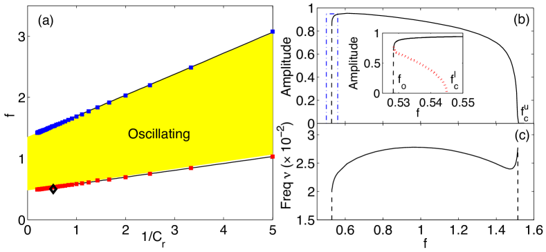
Fig. 1 (a) shows that the system is capable of exhibiting spontaneous oscillation over a range of values of $C_{r}$ and $f$, as has been reported earlier Jacquemet2006 . For a given value of coupling $C_{r}$, the fixed point solution of the system is unstable when $f_{c}^{l}<f<f_{c}^{u}$, where the lower and upper bounds can be obtained analytically by linear stability analysis of Eqs. (1-4) around the steady state. A simple relation between $f_{c}^{l,u}$ and $C_{r}$ is obtained in the limit of large $K$, i.e., when the passive cell relaxes rapidly. Under this condition Eq. (3) is replaced by an algebraic equation such that $\Gamma_{e}=fK(V_{p}^{R}-V_{e})/(1+K/C_{r})$. Thus, as $f$ and $C_{r}$ appear only via $\Gamma_{e}$, the critical value of $f$ depends on $C_{r}$ as $f_{c}^{l,u}=c_{l,u}+m_{l,u}/C_{r}$, where $c_{l,u},m_{l,u}$ are independent of $C_{r}$. Note that, although the above argument is strictly valid only in the large $K$ limit, we observe from our numerical results that the dependence of the critical values of $f$ on $C_{r}$ follows the above relation even for small $K$ [Fig. 1  (a)]. Thus, $f_{c}^{l}(C_{r})$ decreases monotonically with increasing $C_{r}$ and approaches a finite value as $C_{r}\rightarrow\infty$.

While the Hopf bifurcation resulting in loss of stability of the fixed point solution at $f=f_{c}^{u}(C_{r})$ is supercritical, the bifurcation at $f=f_{c}^{l}(C_{r})$ is subcritical so that oscillating solutions of finite amplitude exist for $f<f_{c}^{l}(C_{r})$. For example, for $C_{r}=1.9$ we observe oscillations when $f>f_{c}^{l}=0.545$ [Fig. 1 (b), inset], while they are never observed for $f<f_{0}\simeq 0.529$. Thus, for mean passive cell density in the interval $f_{0}<f<f_{c}^{l}$, the system is multistable so that both fixed point and oscillatory solutions can be observed numerically [see the narrow interval enclosed by the dash-dotted line in Fig. 1 (b)].

In this paper we focus on the situation when $f<f_{c}^{l}(C_{r})$. As discussed in detail later for this condition we observe large fluctuations between replicas when the system is made to undergo dynamical transitions by increasing the coupling between excitable cells, $D$. In contrast, when $C_{r}$ is increased so that $f>f_{c}^{l}(C_{r})$, increasing the coupling $D$ results in a much simpler transition that approaches the mean-field behavior. The replica variations are most pronounced when $f$ just exceeds $\lim_{C_{r}\rightarrow\infty}f_{c}^{l}(C_{r})$, the minimal value of $f_{c}^{l}(C_{r})$. Most of the numerical results reported here are obtained with $f=0.5$ [Fig. 1 (a)], while the minimal value is $f=0.484$.

III.2 Two-dimensional media

Figure 2: Structure of the 2D model system. Excitable cells (large circles) lie on a regular square lattice, and are connected to their neighbors with a coupling strength $D$. In addition, passive cells (small circles) are connected to excitable cells with coupling strength $C_{r}$ at randomly selected sites of the lattice. Each choice of the distribution of passive cells defines a replica.

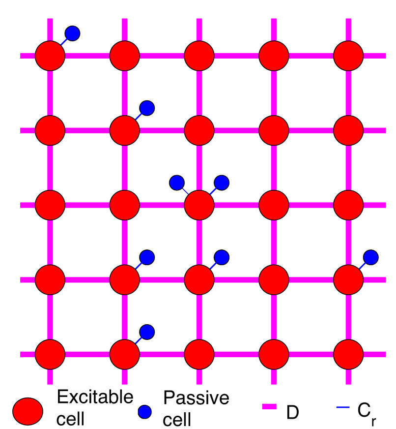
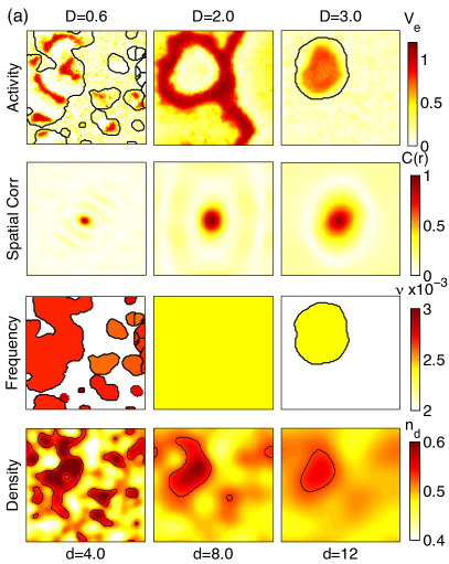
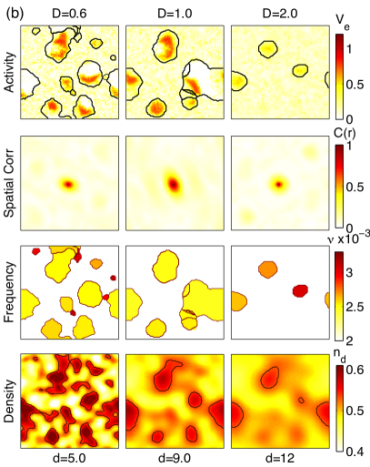
Biological organs exhibiting electrical activity that are often functionally important, such as the heart or the uterus, are spatially extended objects, being made of tissue comprising a large number of excitable and passive cells. As mentioned earlier, we have modeled these by a 2D system of coupled excitable and passive cells with periodic boundaries (Fig. 2). Fig. 3 shows snapshots of activity in two different replicas of such a system as the diffusion constant $D$ is increased. We have investigated the system for a value of the average passive cell density $f=0.5$ and coupling strength between excitable and passive cells $C_{r}=1.9$. For these values, $f<f_{c}^{l}\approx 0.545$, so that in the mean-field limit the medium does not show any oscillation; however, for finite values of $D$, it is possible to observe oscillatory behavior either in local clusters or globally as traveling waves (Fig. 3). We define a non-dimensionalized distance $\mu=(f_{c}^{l}-f)/f_{c}^{l}$ between the system under study and the critical system where the fixed point becomes unstable in the mean-field limit (for $f=0.5$, $\mu\approx 5.7\times 10^{-2}$). For small $\mu$, the behavior of the system is sensitively dependent on the particular replica chosen (Fig. 3). This is manifested as large fluctuations in the system behavior, measured by various order parameters defined later. For example, while global synchronization where all cells oscillate with the same frequency is seen in one replica [Fig. 3 (a), $D=2$], another replica for the same set of parameters exhibits only localized clusters of cells oscillating with different frequencies [Fig. 3 (b), $D=2$].

Figure 3: Replica-dependent fluctuations close to the transition to sustained oscillations in 2D systems of coupled excitable and passive cells, with identical sets of parameters ($f=0.5$, $C_{r}=1.9$, $L=100$), and increasing values of the coupling strength $D$. Snapshots of activity $V_{e}$ for two different replicas are shown in the top rows of (a) and (b). The corresponding time-averaged spatial correlation, which provides a characteristic size of the active regions, is shown in the second row. The frequencies of individual oscillators in the medium are shown in the pseudocolor plots in the third row (white corresponds to absence of oscillation). The last row shows the local density of passive cells averaged over a length scale $d$ indicated below each frame. For the replica shown in (a), we observe global synchronization at $D=2$ followed by progressive cessation of spontaneous periodic activity in the system indicated as a shrinking region of oscillating cells when coupling is increased further. However, for the replica in (b), coherent oscillation is not observed as $D$ is increased, with the existing localized oscillating clusters having distinct frequencies gradually decreasing in size.

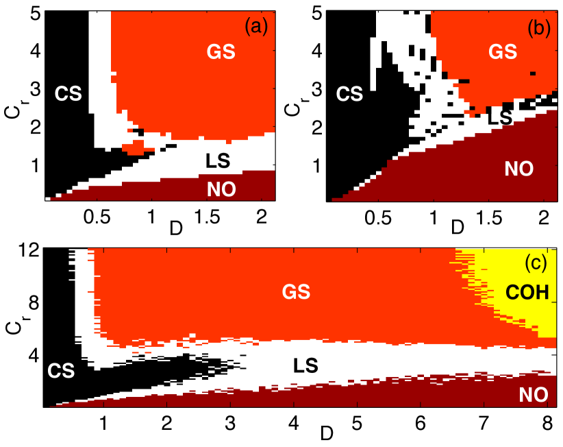
This sensitive dependence of the system dynamics on the distribution of $n_{p}$ can also be seen from the $(D,C_{r})$-parameter space diagrams of the 2D system for different replicas (Fig. 4). While for low values of $C_{r}$, increasing $D$ results in complete absence of oscillations in the system (“No Oscillation” or NO phase), for larger values of $C_{r}$ we observe clusters of oscillating cells (“Cluster Synchronization” or CS phase) at low $D$, with each cluster having a characteristic frequency that may differ from other clusters. As $D$ is increased, the clusters gradually synchronize with each other although isolated regions of non-oscillating cells can exist (“Local synchronization” or LS phase), until all cells eventually oscillate at the same frequency at a sufficiently high $D$ (“Global synchronization” or GS phase). In numerical simulations, the phases were obtained by using suitable order parameters (defined in the next subsection), and choosing appropriate threshold values. As can be seen by comparing Fig. 4 (a) and (b), the diagrams differ quite significantly in terms of the actual dynamical regimes that are observed for the same set of values of $D$ and $C_{r}$, illustrating the significant variability from one replica to the other. By averaging over many such replicas, we can obtain a “mean” phase diagram. The diagram obtained here, Fig. 4 (c), for $f=0.5$ is qualitatively similar to the one obtained in Ref. Singh2012 for a higher value of $f$ (= 0.7). The region corresponding to Coherence or “COH” phase also exists in the present case, appearing at large value of $D$ which is outside the region of interest of the present paper.

Figure 4: (a-b) Phase diagrams for the 2D system of coupled excitable and passive cells with $f=0.5$ in two replicas of linear dimensions $L=50$. Initial values are randomly chosen for each point in the diagram. A “mean” phase diagram obtained by averaging over many ($\sim 100$) replicas is shown in (c) for a system of linear dimension $L=64$. The averaging implies that if a replica is chosen at random for a given $D$ and $C_{r}$, the behavior seen in (c) will be observed with high probability.

III.3 Order parameters

For a detailed quantitative analysis of the spatiotemporal dynamics of the 2D system, we have used two order parameters: (i) the fraction of oscillating cells in the medium $f_{osc}$ and (ii) the width of the frequency distribution as measured by the standard deviation $\sigma_{\nu}$, where $\nu$ denotes the frequencies of the oscillating cells. The amplitude of an oscillating cell is obtained from the square root of the integral of power spectral density (PSD) of the corresponding $V_{e}$ time-series, $\nu$ being the frequency ($>0$) at which the PSD is maximum. The fraction of oscillating cells in the system $f_{osc}=N_{osc}/N$ is the ratio of the number of oscillating cells $N_{\rm osc}$, i.e., those having amplitude higher than a chosen threshold, to the total number of cells $N$. Note that the oscillating cells have approximately the same amplitude which is a consequence of the subcritical nature of the transition across $f_{c}^{l}$ (Fig.1). This enables a clear distinction between oscillating and non-oscillating cells, so that the value of $f_{osc}$ does not depend sensitively on the choice of the threshold.

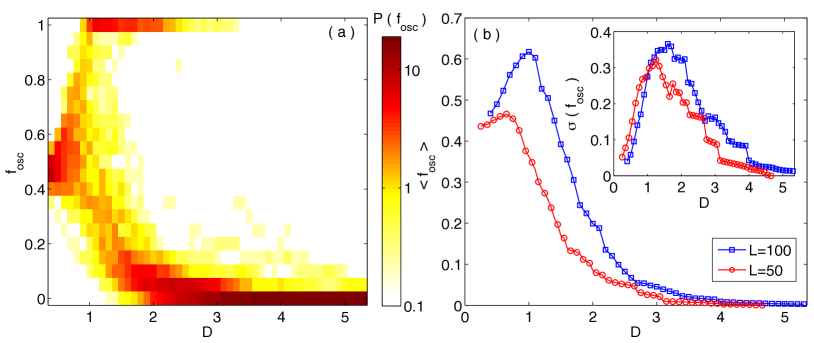
The different phases shown in Fig. 4 are defined in terms of the two order parameters as follows. The LS and GS phases both have $\sigma_{\nu}\rightarrow 0$; however, for the former $f_{osc}<1$ while for the latter $f_{osc}\simeq 1$. The CS phase has a finite $\sigma_{\nu}$ while the NO phase is characterized by $f_{osc}\simeq 0$. The order parameters for a given system depend on the exact form of the quenched spatial disorder and we can investigate the statistical properties of distribution of $f_{osc}$ over an ensemble of replicas (Fig. 5 a). At very low values of $D$, the distribution of $f_{osc}$ is peaked about a value close to $f_{osc}=f$. Upon increasing $D$, the distribution broadens with a bias towards large values of $f_{osc}$. A peak at $f_{osc}=1$ develops around $D\lesssim 1$. Increasing $D$ further, one observes a higher probability for very small values of $f_{osc}$. At $D\lesssim 2$, the distribution has an almost bimodal form, corresponding to realizations with either very few oscillating cells, $f_{osc}\ll 1$, or almost all cells oscillating $f_{osc}\approx 1$. At yet larger values of $D$, the peak at $f_{osc}\approx 1$ disappears, and the distribution concentrates around $f_{osc}=0$, implying a strong reduction in spontaneous activity of the system. This is reflected in Fig. 5 (b), which shows the ensemble average $\langle f_{osc}\rangle$ (where $\langle\rangle$ denotes an averaging over replicas) and the fluctuations about the mean (inset) as a function of the coupling $D$ for 2D systems with $L=50$ and $100$ at $C_{r}=1.9$. We observe that at large values of $D$, the fraction of oscillating cells in the system decreases on average with $D$, and hence is consistent with the mean-field result. The standard deviation of $f_{osc}$ becomes extremely high in the range $1<D<2$ which is a signature of the large fluctuations between different replicas. Comparing between the two curves for $L=50$ and 100 shows that the larger system has a higher probability of showing oscillations than the smaller one for the same parameter values. This dependence on the size of the medium is in fact systematic and is discussed in section V.

Figure 5: (a) Probability distribution function of the fraction of oscillating cells constructed from $176$ different replicas of a 2D system of linear dimension $L=100$, with identical values of $f=0.5$ ($\mu=5.7\times 10^{-2}$), and $C_{r}=1.9$, shown as a function of diffusive coupling strength $D$. (b) Variation of the mean value of $f_{osc}$, and that of the standard deviation (inset) with $D$, both for systems of size $L=100$ (squares) and $L=50$ (circles). Starting from the uncoupled case $D=0$, as the coupling strength becomes larger we observe an increase in the fraction of oscillating cells in the system, in certain cases resulting in global synchronization. Further increase of the coupling eventually leads to complete cessation of any activity in the system. The fluctuation about the mean is maximum at $D\lesssim 2$ (inset), when the distribution exhibits a strong bimodal nature.

IV Fluctuations of passive cell density and local activity

The behavior described in the previous section can be qualitatively understood by noticing that diffusion effectively couples excitable cells that are within a distance $\propto\sqrt{D}$ of each other. As a consequence, one can expect that the behavior of a given excitable cell depends on the density of passive cells in its neighborhood characterized by the distance $\sqrt{D}$. With this motivation, we begin by describing the procedure for computing the local density of passive cells surrounding a given excitable cell.

IV.1 Averaging procedure

We define local passive cell density ${\bar{n}}_{d}$ coarse-grained over a length scale $d$ as the convolution ${\bar{n}}_{d}=K_{d}*n_{p}$ of the spatial distribution of passive cells $n_{p}(i,j)$ ($i,j=1,\ldots,L$) over the lattice with a 2D averaging kernel $K_{d}(i,j)$. For simplicity we have considered separable kernels, i.e., $K_{d}(i,j)=k_{d}(i/d)\times k_{d}(j/d)$. As the coupling term is effectively described by a Laplacian, a natural choice for the coarse-graining kernel $K_{d}$ is the Gaussian kernel $K^{G}_{d}$ given by:

$$k^{G}_{d}(i)=\frac{1}{\sqrt{2\pi d^{2}}}\exp(-\frac{i^{2}}{2d^{2}})\,,$$ (5)

which has been used for the numerical investigation of the model system presented in this section. For analytical convenience we have also used the simpler “square top hat” kernel, $K^{STH}_{d}$ in section V which is based on the classical 1D top hat filter:

$$k^{TH}_{d}(i)=\frac{1}{d}H(d/2-|i|)\,,$$ (6)

where $H(.)$ is the Heaviside step function, i.e. $H(x)=0$ when $x\leq 0$ and $H(x)=1$ otherwise. For the square top hat kernel, ${\bar{n}}_{d}(i,j)$ is the number of passive cells, averaged over a square subregion of size $N_{d}=d^{2}$ centered at the point $(i,j)$. In the case of the Gaussian kernel $K^{G}_{d}$, the contribution from a site $(i^{\prime},j^{\prime})$ to $n_{p}$ at site $(i,j)$ depends on the distance between the two. The variance of ${\bar{n}}_{d}$ can be written as $\sigma_{d}^{2}=\sigma^{2}/N_{d}$, where $\sigma^{2}$ is the variance of $n_{p}$, and $N_{d}$ ($=4\pi d^{2}$) is the effective number of sites contributing to ${\bar{n}}_{d}$.

IV.2 Emergence of pacemaker-like regions through diffusion

As can be seen from Fig. 3, large-amplitude oscillations occur in regions that have the highest local density of passive cells. In addition, the features observed on increasing the diffusion coefficient $D$ resemble the patterns of the local passive cell density seen upon increasing the averaging size $d$. As $f<f_{c}^{l}$, increasing $D$ is expected to ultimately suppress oscillation in Fig. 3 in agreement with the mean-field analysis. Indeed, we observe that at larger values of $D$, the number of oscillating cells is reduced on average. The coarse-graining procedure reflects this phenomenon as with increased kernel width $d$ the variations in $\bar{n}_{d}$ are reduced significantly. This decreases the probability that a cell will have sufficiently high local passive cell density to generate oscillations.

We define a “pacemaker-like region” to be a group of adjacent cells with a local passive cell density $\bar{n}_{d}$ larger than the threshold $f_{c}^{l}(C_{r})$. The oscillatory activity arising in these regions may propagate in the form of waves to the rest of the system, so that they effectively act as pacemakers that are seen in systems having specialized coordination centers.

The number of cells comprising the pacemaker-like region varies from replica to replica. When $f<f_{c}^{l}$, we expect the size of the region to shrink with increasing coarse-graining length $d$, eventually disappearing at large $d$ (as predicted by mean-field analysis). Thus, for a given replica, we can measure the largest value of the coarse-graining length, $d^{*}$, for which a pacemaker-like region still exists. This is the smallest value of $d$ for which $\bar{n}_{d}<f_{c}^{l}$ everywhere in the 2D system.

Figure 6: Relation between the largest values of coarse-graining length $d^{*}$ and diffusion coefficient $D^{*}$ for which a given 2D system possesses regions with oscillatory activity. Each point corresponds to a different replica whereas different symbols represent different system sizes $N=L^{2}$. Error bars centered around averages of replicas for the same system size express the standard deviation. The linear fit between $d^{*2}$ and $D^{*}$, shown as a broken line, has a slope $T\simeq 36.6$ that lies in the middle of the range of observed oscillation periods (lying between $31$ and $40$) for different values of the diffusive coupling strength in a 2D system with $L=50$.

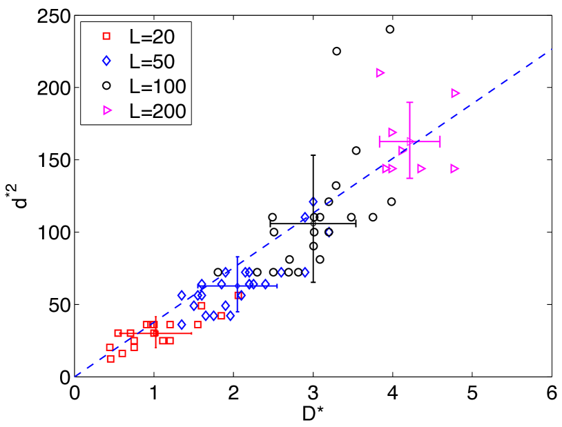
As mentioned above, the coarse-graining length $d$ is related to the diffusion coefficient $D$, expected to be of the form $d\sim\sqrt{D}$. Therefore, in analogy with $d^{*}$, we can define a value $D^{*}$ of the diffusion coefficient above which the number of oscillating cells in the system goes to zero. Fig. 6 demonstrates that the relation between $d^{*}$ and $D^{*}$ (shown for different replicas and system sizes) follows $d^{*2}\approx TD^{*}$, where $T$ is the slope of the linear fit and defines a characteristic time of the order of the slow time scale in the system, $\sim 1/\epsilon$. We note that as system size increases, both $D^{*}$ and $d^{*}$ increase. Thus, for systems just below the critical threshold for oscillatory activity, i.e., $f\leq f_{c}^{l}$, oscillations are seen for a wider range of $D$ in larger systems. This size dependence is investigated quantitatively in section V.

V Statistical description

In this section, we investigate the effect of coarse-graining length $d$ on the presence and spatial extent of pacemaker-like regions in the 2D system. For analytical convenience, we use the ‘square top hat’ kernel, Eq. (6), for coarse-graining.

V.1 Distribution of passive cells

Consider a 2D lattice with $N=L^{2}$ excitable cells in which a total number of $M=f~{}N$ passive cells are randomly distributed. The probability that there are $N_{p}$ passive cells in a region containing $N_{d}=\zeta N$ ($0<\zeta<1$) excitable cells is given by the binomial distribution:

$$p^{N}_{N_{d}}(N_{p})=\binom{M}{N_{p}}\zeta^{N_{p}}(1-\zeta)^{M-N_{p}}.$$ (7)

When $N\rightarrow\infty$, this reduces to a Poisson distribution with mean $fN_{d}$ :

$$p^{\infty}_{N_{d}}(N_{p})=\frac{(fN_{d})^{N_{p}}e^{-fN_{d}}}{N_{p}!}.$$

For a square top hat kernel, the averaging occurs over $N_{d}=d^{2}$ sites where $d$ is the coarse-graining length and the local passive cell density ${\bar{n}}_{d}=N_{p}/N_{d}$. For a Gaussian kernel, the corresponding coarse-grained region comprises $N_{d}=4\pi d^{2}$ sites.

V.2 Probability of the occurrence of a spontaneously oscillating cell in a neighborhood of $N_{d}$ cells

Given the probability distribution of passive cells, we now determine the probability that a given cell is capable of spontaneous oscillations when it is effectively coupled through diffusion to a neighborhood consisting of $N_{d}$ cells. This is obtained by considering the probability that the local passive cell density $\bar{n}_{d}=N_{p}/N_{d}\geq f_{c}^{l}$, which is given by the cumulative distribution corresponding to Eq. (7):

$$P^{N}_{N_{d}}=\sum_{N_{p}=f_{c}^{l}N_{d}}^{M}p^{N}_{N_{d}}(N_{p})=I_{\zeta}(f_{c}^{l}N_{d},M-f_{c}^{l}N_{d}+1),$$ (8)

where $I_{x}(a,b)$ is the regularized (incomplete) beta function Cramer:57 and $P^{N}_{N_{d}}$ depends on system size $N$. In the limit ${N\rightarrow\infty}$, $P^{N}_{N_{d}}$, tends to a regularized incomplete gamma function Abramowitz:72 ,

$$P^{\infty}_{N_{d}}=\frac{\gamma(f_{c}^{l}N_{d},fN_{d})}{\Gamma(f_{c}^{l}N_{d})}.$$ (9)

The probabilities obtained for different values of $N_{d}$ from the above expression agrees well with the corresponding values numerically obtained from different replicas of the 2D system in Fig. 7.

In the limit of large system size $N$, $P^{\infty}_{N_{d}}$ can be rewritten by expressing the incomplete beta function in Eq. (8) as a continuous fraction Abramowitz:72 and keeping only lower order terms in $N_{d}^{-1}$ and $N^{-1}$. In addition, neglecting $\zeta=N_{d}/N$ we obtain for any fixed value of $\mu$:

$$P^{\infty}_{N_{d}}\simeq\frac{1}{\sqrt{2\pi f_{c}^{l}N_{d}}}\frac{{\rm e}^{-\lambda f_{c}^{l}N_{d}}}{\mu}\,,$$ (10)

where $\lambda=-\mu-\log(1-\mu)$. This expression can also be obtained from Eq. (9) by expanding the regularized incomplete gamma function and using the Stirling approximation. For small $\mu$, we have $\lambda\simeq\mu^{2}/2>0$ and on introducing a reduced variable ${\cal X}=\mu^{2}f_{c}^{l}N_{d}$ one obtains:

$$P^{\infty}_{N_{d}}\simeq\frac{{\rm e}^{-{\cal X}/2}}{\sqrt{2\pi{\cal X}}}\,.$$ (11)

Figure 7: Probability $P^{N}_{N_{d}}$ of having local passive cell density greater than $f_{c}^{l}$ in a neighborhood of $N_{d}$ excitable cells as a function of $N_{d}$. Open (filled) symbols represent numerical observations using Gaussian (square top hat) kernel. The broken curves indicate the corresponding probabilities obtained from the analytical expression of $P^{N}_{N_{d}}$, Eq. (8). The solid curve shows $P^{\infty}_{N_{d}}$, the probability values obtained for infinitely large system, Eq. (9).

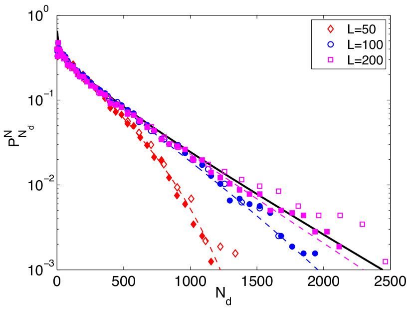
Note that in order to ensure that all replicas for a given value of $f$ have exactly the same mean number of passive cells $f=\bar{n}_{p}$ connected to an excitable cell, we have used a binomial distribution of $n_{p}$ for generating the different replicas in our numerical study. In comparison, the Poisson distribution used in our analysis leads to a mean fraction of passive cells attached to an excitable cell that varies from one replica to another for a given value of $f$. In the limit of large system size, the fluctuations in the number of passive cells become very small, so that both binomial and Poisson distributions lead to the same behavior. However, when $N$ is not very large, these fluctuations are appreciable when using the Poisson distribution which introduces biases in the results (see Figs. 7 and 9). In addition, for finite $N$, corrections of order $N_{d}/N$ are expected in the expression involving the reduced variable $\cal{X}$, Eq. (11). These effects are responsible for deviations between the predictions of our analysis and the numerical results.

V.3 Probability of the occurrence of a pacemaker-like region in the 2D system

As mentioned earlier, Fig. 6 shows $d^{*}$, the largest value of the coarse-graining length $d$ for which a pacemaker-like region exists in the 2D system, as a function of the diffusion coefficient. We define the probability $\Pi^{N}_{N_{d}}$ of having a pacemaker-like region in the system as the probability of having at least one cell with $\bar{n}_{d}\geq f_{c}^{l}$ in a replica of size $N=L^{2}$ cells when the coarse-graining is done over a neighborhood of $N_{d}$ cells. Fig. 8 shows the sigmoid form of this probability as a function of $N_{d}$, computed by using 400 replicas. To obtain an effective value of $d^{*}$ (or $N_{d}^{*}$) for an ensemble of many replicas, we define the quantity $\tilde{d}^{*}$ (or $\tilde{N}_{d}^{*}$) by the condition that $\Pi^{N}_{\tilde{N}_{d}^{*}}=1/2$. As mentioned earlier, larger systems have higher probability of having a pacemaker-region for a fixed value of $d$ (or $N_{d}$) which is explicitly shown in Fig. 8.

Figure 8: Probability $\Pi^{N}_{N_{d}}$ of having a pacemaker-like region in a 2D system of size $N=L^{2}$ as a function of the coarse-graining size $N_{d}$. Different symbols represent different systems sizes from $L=50$ to 6400. The continuous lines indicate fits to the theoretical expression for $\Pi^{N}_{N_{d}}$ given by Eq. (12).

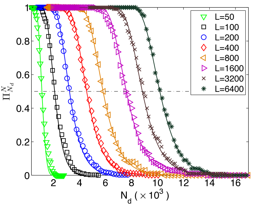
If we assume that there are $\eta$ uncorrelated, i.e. effectively independent, subsets of size $N_{d}$ in the 2D system, we have:

$$\Pi^{N}_{N_{d}}=1-\left(1-P^{N}_{N_{d}}\right)^{\eta}.$$ (12)

One possible estimate of $\eta$ is to assume that the independent subsets are obtained by tiling the system using non-overlapping blocks of size $N_{d}$, i.e., $\eta=N/N_{d}$. However, a single pacemaker region may be split among several neighboring tiles, which effectively leads to an underestimation of the probability $\Pi^{N}_{N_{d}}$. Another possible estimate of $\eta$ is to assume that all blocks of size $N_{d}$ are independent, so that $\eta=N$. However, the high degree of overlap between neighbouring blocks introduces significant correlations between them, leading to an overestimation of $\Pi^{N}_{N_{d}}$ in Eq. (12).

In general, we expect that the value of $\eta$ will be related to $N$ and $N_{d}$ by $\eta=m\cdot N/N_{d}$. The existence of a number $m$ independent of the system size can be qualitatively understood from the following argument. Consider the covariance of the two variables, $f_{d}(i,j)=N_{p}(i,j)/N_{d}$ and $f_{d}(i^{\prime},j^{\prime})$, i.e., of the average number of passive cells at the two sites $(i,j)$ and $(i^{\prime},j^{\prime})$ separated by a distance $l=\sqrt{(i-i^{\prime})^{2}+(j-j^{\prime})^{2}}$. It has the exact expression $\sigma\rho(l)/N_{d}$ where $\sigma=(1-\zeta)f$ and $\rho(l)=\exp[-(l/2d)^{2}]$ is the correlation between the two sites. Thus, how fast the two values of $f_{d}$ decorrelate is simply given by $\rho(l)$. To estimate the number of independent subsets containing $N_{d}$ points, we introduce $\kappa$, defined as the maximum possible correlation between two independent subsets. The correlation length $l_{0}$ is then defined by $\rho(l_{0})=\kappa$, so that two subsets separated by a distance $l>l_{0}$ are independent. This implies the existence of $N/l_{0}^{2}$ independent blocks, suggesting in turn that $m=N_{d}/l_{0}^{2}$. Intuitively, one expects $l_{0}$ to be of the order of the width of the Gaussian kernel, $d$, yielding $m\approx 4\pi$. We have numerically obtained the effective number $m$ by least-square fitting of the numerical data shown in Fig. 8 with the theoretical expression of Eq. (12). This gives values of $m$ lying in the range $9.5\leq m\leq 16.5$, which is in fact consistent with the heuristic estimate $m=4\pi$.

V.4 System size dependence of the probability of occurrence of pacemaker-like region

We now obtain the cutoff value $N_{d}^{*}$ for the coarse-graining size below which oscillations are present in the system by solving

$$\Pi^{N}_{N_{d}^{*}}=1-\left(1-P^{N}_{N_{d}^{*}}\right)^{m\frac{N}{N_{d}^{*}}}=1/2.$$ (13)

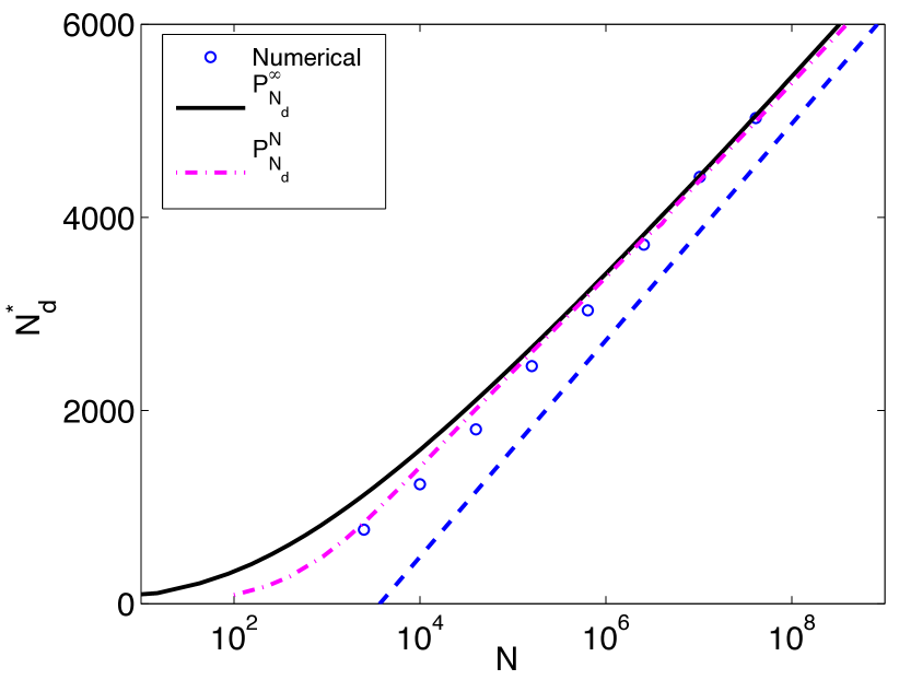
To solve this equation, we assume that the system is large enough, so that $P^{N}_{N_{d}^{*}}$ can be replaced by $P^{\infty}_{N_{d}^{*}}$, Eq. (10). This implies that the only system-size dependence of $\Pi^{N}_{N_{d}}$ is from the exponent $mN/N_{d}$. We thus obtain a linear relation between $\log(N)$ and $N_{d}^{*}$ (Fig. 9):

$$\mu^{2}f_{c}^{l}N_{d}^{*}=2\log N+2\log\frac{\mu^{2}f_{c}^{l}m}{\log(2)\sqrt{2\pi}},$$ (14)

which effectively defines $N_{d}^{*}$. For large systems, the behavior of $N_{d}^{*}$ is well described by the $\log(N)$ term in Eq. (14) shown by a straight line in Fig. 9. It is worth noting that the $\log(N)$ scaling appears very naturally in the general context of extreme value statistics Maj_JSP_2005 . The constant term in the R.H.S. of Eq. (14) is responsible for the deviations from $\log(N)$ scaling seen for $N\lesssim 10^{4}$.

Figure 9: The largest coarse-graining size for which oscillations are observed in the system, $N_{d}^{*}$, defined as $\Pi^{N}_{N_{d}^{*}}=1/2$, as a function of the system size $N$. The circles represent numerical data shown in Fig. 8. The dashed straight line is a guide to the eye indicating the slope $1/(\lambda f_{c}^{l})$. The solid line and dashed-dotted line represent the solutions of Eq. (13) using the expressions given by Eq. (8) and Eq. (9) respectively.

VI Scaling in the transition to activity in spatially extended systems

Figure 10: (a) Average value and (b) standard deviation of the fraction of oscillating cells in a 2-D system, shown as a function of the reduced variable $4\pi DT/N_{d}^{*}$, where $N_{d}^{*}$ is defined in Eq. (14). The symbols indicated in the legend correspond to different values of $L$ and $f$, i.e., $N$ and $\mu$. The different curves collapse to the same form (within statistical accuracy) when $N_{d}$ is large, the regime for which the analysis described in the text is valid.

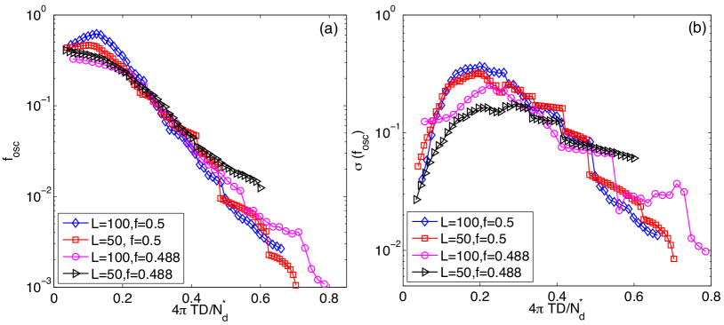
The analysis presented in the previous section allows us to identify a characteristic coarse-graining size, suggesting that the number of pacemaker-like regions in a given system is determined by the ratio $N_{d}/N_{d}^{*}$, where $N_{d}^{*}$ is given by Eq. (14). In addition, Fig. 6 shows that diffusive coupling $D$ results in coarse-graining of the passive cell density over a region of size $N_{d}\approx 4\pi DT$, with $T$ being the typical oscillation period (subsection IV.2). Based on this, we expect that the fraction of oscillating cells will depend on the reduced variable $4\pi DT/N_{d}^{*}$.

Fig. 10 shows the average (a) and the standard deviation (b) of the fraction of oscillating cells, $f_{osc}$, averaged over many ($\sim 100$) replicas as a function of $4\pi DT/N_{d}^{*}$, for several values of $f$ (or equivalently, of $\mu$) and $L$. The curves for the mean value of $f_{osc}$ seem to collapse to a common form at large $N_{d}$ where our analysis applies, Eq. (10), is not valid when $N_{d}$ is small; see in particular the discussion at the end of subsection V.2), supporting the conclusion that the properties of the system indeed vary with the scaling parameter $D/N_{d}^{*}$. The deviations seen in the different curves can be explained as an outcome of the large standard deviation in $f_{osc}$ as seen from Fig. 10 (b). Remarkably, apart from the curves corresponding to the average values, we also observe relatively good collapse in the curves corresponding to the standard deviation of $f_{osc}$, at least when $D/N_{d}^{*}$ is not too small. This suggests that our analysis may apply not only to the averaged value, but also to the second moment of the distribution of the fraction of oscillating cells, $f_{osc}$.

As mentioned in the previous section, in the limit of very large system size, $N_{d}^{*}$ is a function of the reduced variable $\mu^{2}D/\log(N)$. This scaling implies that for a fixed value of the coupling between excitable cells, as system size is increased and/or the mean value $f$ of the passive cell distributions comes closer to the critical value $f_{c}^{l}$, there is higher probability of observing sustained oscillatory activity in the system. Alternatively, if $f$ is kept fixed at a value smaller than $f_{c}^{l}$, then the larger the system size, the larger the range of values of $D$ over which oscillations can be observed.

VII Conclusion

In this paper we explore the role of heterogeneity in the spatial distribution of passive cells, which introduces quenched disorder in a system of coupled excitable and passive cells, on the transition between quiescent state and oscillatory activity. We begin our analysis with the mean-field limit of the spatially extended system, which is equivalent to a single excitable cell coupled to a number of passive cells. We observe here that the transition from quiescent to oscillatory activity is subcritical, i.e., oscillations appear at onset with a finite amplitude. We next investigate the system at finite values of the coupling between excitable cells and characterize the coarse-graining effect of diffusion. We show that the dynamical behavior of the system is related to the local passive cell density obtained using a suitable coarse-graining length scale. We observe large variability in the dynamical behavior of different replicas, i.e., different realizations of the spatial distribution of passive cells. The strong effect of this quenched disorder on the dynamics is reminiscent of glassy systems. To characterize the properties averaged over many realizations of the disorder, we assume that the effect of diffusion of strength $D$ is to coarse-grain the local passive cell distribution over $N_{d}$ sites. We indeed empirically establish that $D\propto N_{d}$. From this perspective, we analyze the transition between quiescent state and sustained oscillations. We obtain a scaling relation that describes the transition as a function of (i) system size, (ii) coupling between excitable cells and (iii) average passive cell density. One of the important implications of this relation is that the occurrence of oscillatory behavior depends on the logarithm of the system size $N$ so that increasing $N$ enhances the probability of observing oscillations.

As mentioned in the introduction, the model system that we have analyzed has been motivated by the biological phenomenon of onset of coherent oscillations in the pregnant uterus close to term. One of the implications of our work is that larger organs may show greater variability in their dynamical behavior for a given set of parameters describing the state of the system. In particular, they may be more likely to exhibit oscillations even prior to the transition point as a result of spatial fluctuations, potentially implying that mammals having bigger uteri will be at higher risk of having pre-term rhythmic activity. As it is not yet well-understood why in some cases periodic dynamical behavior is initiated in uterine tissue significantly earlier than normal, our study of the role of disorder in creating an effective pacemaker-like region giving rise to rhythmic activity in such systems may be of potential significance for possible clinical applications. Our work also connects the dynamical phenomena seen in such biological systems with the study of the role of disorder in phase transitions occurring in several physical systems, including spin glasses.

We are grateful to E. Bertin, P. Leboeuf and S. Majumdar for insightful discussions. We thank the HPC facility (IMSc) and the PSMN (ENS Lyon) for providing computer resources. This research was supported in part by IFCPAR (Project No. 3404-4).

References

- (1) L. Glass, Nature (Lond.) 410, 277 (2001).
- (2) C. H. Orchard, D. A. Eisner and D. G. Allen, Nature (Lond.) 304, 735 (1983).
- (3) A. Goldbeter, Biochemical Oscillations and Cellular Rhythms (Cambridge Univ. Press, Cambridge, 1997).
- (4) E. Grapengiesser, E. Gylfe and B. Hellman, Biochem. Biophys. Res. Commun. 151, 1299 (1988).
- (5) G. Buzsáki and A. Draguhn, Science 304, 1926 (2004).
- (6) A. T. Winfree, The Geometry of Biological Time (Springer, New York, 2000).
- (7) M. Golubitsky, I. Stewart, P.-L. Buono and J. J. Collins, Nature (Lond.) 401, 693 (1999).
- (8) R. W. Tsien, R. S. Kass and R. Weingart, J. Exp. Biol. 81, 205 (1979).
- (9) J. Keener and J. Sneyd, Mathematical Physiology (Springer, New York, 1998).
- (10) D. P. Zipes and J. Jalife, Cardiac Electrophysiology: From Cell to Bedside (Saunders-Elsevier, Philadelphia, 2009).
- (11) T. R. Chigwada, P. Parmananda and K. Showalter, Phys. Rev. Lett. 96, 244101 (2006).
- (12) A. Shmygol, A. M. Blanks, G. Bru-Mercier, J. E. Gullam and S. Thornton, Ann. N.Y. Acad. Sci. 1101, 97 (2007).
- (13) R. Duquette, A. Shmygol, C. Vaillant, A. Mobasheri, M. Pope, T. Burdyga and S. Wray, Biology of Reproduction 72, 276 (2005).
- (14) L. M. Popescu, S. M. Ciontea and D. Cretoiu, Ann. N.Y. Acad. Sci. 1101, 139 (2007).
- (15) V. Jacquemet, Phys. Rev. E 74, 011908 (2006).
- (16) A. Kryukov, V. S. Petrov, L. S. Averyanova, G. V. Osipov, W. Chen, O. Drugova and C. K. Chan, Chaos 18, 037129 (2008).
- (17) W. Chen, S. Cheng, E. Avalos, O. Drugova, G. Osipov, P.-Y. Lai and C. K. Chan, EPL 86, 18001 (2009).
- (18) J. H. E. Cartwright, Phys. Rev. E 62, 1149 (2000).
- (19) V. S. Petrov, G. V. Osipov and J. Kurths, Phys. Rev. E 82, 026208 (2010).
- (20) R. C. Young, Ann. N.Y. Acad. Sci. 1101, 72 (2007).
- (21) R. Young and R. Hession, Obstetrics Gynecology 93, 94 (1999).
- (22) S. M. Miller, R. E. Garfield and E. E. Daniel, Am. J. of Physiol. Cell Physiol. 256, C130 (1989).
- (23) H. Miyoshi, M. Boyle, L. MacKay and R. Garfield, Biophys. J. 71, 1324 (1996).
- (24) R. Garfield, G. Saade, C. Buhimschi, I. Buhimschi, L. Shi, S. Shi and K. Chwalisz, Human Reproduction Update 4, 673 (1998).
- (25) R. Singh, J. Xu, N. G. Garnier, A. Pumir and S. Sinha, Phys. Rev. Lett. 108, 068102 (2012).
- (26) A. Pumir, A. Arutunyan, V. Krinsky and N. Sarvazyan, Biophys. J. 89, 2332 (2005).
- (27) V. S. Petrov, G. V. Osipov and J. A. K. Suykens, Phys. Rev. E 79, 046219 (2009).
- (28) G. Bub, A. Shrier and L. Glass, Phys. Rev. Lett. 88, 058101 (2002).
- (29) G. Bub, A. Shrier and L. Glass, Phys. Rev. Lett. 94, 028105 (2005).
- (30) K. Binder and A. P. Young, Rev. Mod. Phys. 58, 801 (1986).
- (31) M. Mézard, G. Parisi and M. A. Virasoro, Spin Glass Theory and Beyond (World Scientific, Singapore, 1987)
- (32) S. Baer and T. Erneux, SIAM J. Appl. Math. 52, 1651 (1992).
- (33) M. Ringkvist and Y. Zhou, Nonlinear Analysis 71, 2667 (2009).
- (34) P. Kohl, A. G. Kamkin, I. S. Kiseleva and D. Noble, Experimental Phyisology 79, 943 (1994).
- (35) H. Cramér, Mathematical Methods of Statistics (Princeton University Press, Princeton, 1957)
- (36) M. Abramowitz and I. A. Stegun, Handbook of Mathematical Functions With Formulas, Graphs, and Mathematical Tables (Dover, New York, 1972)
- (37) S. N. Majumdar and A. Comtet, J. Stat. Phys. 119, 777 (2005).