Automatic spin-entangled decays of heavy resonances in Monte Carlo simulations

Abstract:

We present a general method that allows one to decay narrow resonances in Les Houches Monte Carlo events in an efficient and accurate way. The procedure preserves both spin correlation and finite width effects to a very good accuracy, and is therefore particularly suited for the decay of resonances in production events generated at next-to-leading-order accuracy. The method is implemented as a generic tool in the MadGraph5 framework, giving access to a very large set of possible applications. We illustrate the validity of the method and the code by applying it to the case of single top and top quark pair production, and show its capabilities on the case of top quark pair production in association with a Higgs boson.

1 Introduction

The analysis of scattering processes involving heavy resonances at the Large Hadron Collider (LHC) is of essential importance. One of the reasons is that the Higgs boson couples primarily to heavy particles such as the top quark and the weak bosons. Also many theories beyond the Standard Model predict the existence of unstable particles at the TeV scale. These unstable particles are not observed directly, but they initiate a cascade of decays (also called a decay branch) ending up with particles that may be observed in the detector. Such processes lead to a rich phenomenology, because the spin of the heavy resonances and the type of coupling to other fields imply non-trivial angular correlations among the final-state particles inside a given decay branch (a phenomenon also called decay spin correlation effects) or among the particles from distinct decay branches (a phenomenon also called production spin correlation effects).

Nowadays virtually all experimental analyses at the LHC rely on tools to simulate scattering events and their reconstruction in the detector. As Monte Carlo generators have become an increasingly important tool for collider physics, a large effort has been devoted to improving their accuracy, in particular, by developing parton-level generators based on next-to-leading-order (NLO) QCD matrix elements. In this respect, the simulation of production events with heavy resonances at next-to-leading-order accuracy in QCD is particularly challenging, because the decay pattern of these resonances may lead to signatures characterized by a large particle multiplicity in the final state. Because of the intrinsic complexity of next-to-leading-order amplitudes for large multiplicities of external particles, the efficiency of the current algorithms imposes some limitations on the range of possible applications. In many instances, some approximations must be made, otherwise the generation of events cannot be handled in practice.

In this context, one well-known simplification is the narrow width approximation, which delivers a good accuracy in the case of a resonance with a width $\Gamma$ much smaller than its mass. In this approximation, intermediate resonances are put on their mass shell, significantly simplifying the structure of QCD corrections since radiative corrections in the production and in the decay do not interfere in the limit $\Gamma\rightarrow 0$. As a result, QCD corrections in the production and in the decay can be handled separately. This scheme is implemented in Monte Carlo integrators such as MCFM [1, 2, 3] for specific processes involving the top quark. In that implementation, spin correlation effects are retained at next-to-leading-order accuracy (in the limit $\Gamma\rightarrow 0$).

However, as far as Monte Carlo event generators are concerned, the previous approach may not be the optimal one. Indeed, in the case of processes with complicated decay patterns, the efficiency of the generation of unweighted events (i.e. events with the same weight) becomes a serious issue. This problem of efficiency may be overcome by considering a stronger assumption, sometimes called the decay chain approximation [4] which consists of factorizing the squared amplitude into a production factor and a decay factor. Using this scheme, the generation of unweighted events can be split into (1) the generation of undecayed events in which these resonances appear as on-shell final state particles and (2) the decay of the resonances in each production events. Off-shell effects may partly be recovered by smearing the invariant mass of each heavy resonance according to a Breit-Wigner distribution, and by reshuffling the other momenta in the undecayed event. In the simplest implementation of this scheme, each resonance is decayed according to a uniform distribution in its rest frame, in which case spin correlation effects are lost. To gain accuracy, kinematics of the decay products can be generated randomly according to the squared amplitudes for the decay processes [5]. In this latter case, decay spin correlation effects are partially preserved, while production spin correlation effects are lost as a result of the production vs. decay factorization at the squared amplitude level.

In the search for the optimal approach to generate events with intermediate resonances, a compromise must be reached between the efficiency and the accuracy of the approach. In this spirit, Frixione, Laenen, Motylinski and Webber [6] have proposed a convenient procedure (called the FLMW procedure in this paper) for Monte Carlo generators which not only preserves the efficiency inherent to the decay chain approximation, but also includes nearly all spin correlation effects at next-to-leading-order accuracy. They implemented this scheme in MC@NLO [7, 8] and in Powheg [9] for specific processes involving the production of top quarks and weak bosons. The accuracy of the scheme was demonstrated for these processes.

Since the work of Frixione et al, there has been a tremendous progress in automating next-to-leading-order calculations. A new milestone has been reached by promoting Monte Carlo generators into the era of fully automated NLO event generators [10, 11, 12]. This breakthrough has opened various interesting perspectives on hadron collider phenomenology, by allowing the simulation of a new class of processes at next-to-leading-order accuracy. Among these processes, the production of heavy resonances –such as top quark pair production in association with a Higgs boson [11, 13]– are directly relevant for the ongoing phenomenology at the Large Hadron Collider. Even though these automated NLO Monte Carlo generators feature, in principle, no restrictions on complexity of the process and particle multiplicity, in practice the CPU cost becomes enormous for high-multiplicity final states. Most of the current tools cannot simulate the full production and decay at NLO accuracy in a reasonable amount of time; only the generation of undecayed events at next-to-leading order is feasible.

Some frameworks already exist to decay heavy resonances in undecayed events. However the existing tools are either limited to specific processes (e.g. the implementation in MC@NLO [6]), or they do not provide an acceptable accuracy given the current state-of-the-art of simulation techniques (e.g. the program BRIDGE [5] or the generic decay routines in Pythia [14, 15] or Herwig [16]). In this work, we provide a generic and accurate algorithm to decay heavy resonances in undecayed events generated at next-to-leading-order accuracy. We revisit the FLMW procedure and we demonstrate that this procedure can be fully automated. Special care is taken to handle the off-shell effects and the reshuffling of the momenta. We implement this algorithm in the MadGraph5 framework [17] and we dub this new tool MadSpin.

2 Spin correlations in the decay

We start by introducing some notation. The kinematics $X$ of an event $E_{X}$ can be parametrized by a set of independent variables $\textbf{x}=x^{1},\dots,x^{r}$ each of them in the range $[0,1]$. The function $\phi:\textbf{x}\rightarrow X$ that maps the variables x onto the kinematics $X$ is usually called phase-space mapping. In the corresponding decayed event $E_{X_{\textrm{dk}}}$ (with corresponding kinematics $X_{\textrm{dk}}$) an additional set of independent variables $\textbf{y}=y^{1},\dots,y^{s}$ is needed to parametrize the kinematics of the decay products. In this work, the variables y for each resonance decay are always in one-to-one correspondence with the invariant mass of the resonance and the angles defining the direction of the decay products in the rest frame of the resonance.

Next-to-leading-order generators typically produce a list of events, where each event $E_{X}$ is characterized by the fully exclusive kinematics $X$. The FLMW procedure [6] allows one to generate the decays of narrow resonances in the event $E_{X}$ according to distributions that retain both decay and production spin correlation effects. For each undecayed event, the procedure goes as follows.

1. The variables y characterizing the decay of the resonances are generated randomly, considering –for each decay– a uniform distribution of the decay products in the rest frame of the decaying particle, and the decayed event with kinematics $X_{\textrm{dk}}(\textbf{x},\textbf{y})$ built upon these variables is reconstructed.

2. The differential cross section $d\sigma/d\textbf{x}d\textbf{y}$ associated with the decayed process is evaluated with tree-level matrix elements at the decayed event with kinematics $X_{\textrm{dk}}(\textbf{x},\textbf{y})$ and an unweighting procedure with respect to the maximum weight is used to decide whether this decayed event should be kept or not. More precisely, if $W_{\textrm{max}}(X)$ represents the maximum value of the differential cross section over the range of possible decay configurations y’s, a random number $r$ is generated uniformly between 0 and 1, and the decayed event $X_{\textrm{dk}}(\textbf{x},\textbf{y})$ is retained provided that the condition

   $$\frac{d\sigma}{d\textbf{x}d\textbf{y}}\left(X_{\textrm{dk}}(\textbf{x},\textbf{y})\right)>rW_{\textrm{max}}(X)$$ (1)

   is satisfied. Otherwise the procedure to decay the event with kinematics $X$ is restarted from step 1 onwards. This ensures that a decayed event $X_{\textrm{dk}}(\textbf{x},\textbf{y})$ is kept with a probability that is proportional to the differential cross section evaluated at this event.

It should be emphasized that only tree-level amplitudes are used when evaluating differential cross sections in the FLMW procedure. For production events with an extra hard radiation, spin correlation effects are included at next-to-leading-order accuracy. For the other events, spin correlation effects are included at leading order accuracy, as no information on the one-loop corrections not factorizing the Born is used to generate the decay configurations.

Frixione et al. also recognized that, in the narrow width approximation, the maximum weight $W_{\textrm{max}}(X)$ can be expressed as a product of the differential cross section for the undecayed process $d\sigma_{\textrm{no-dk}}/d\textbf{x}$ evaluated at $X$ and a constant factor $W^{\textrm{dk}}$ that is independent of the undecayed event $E_{X}$:

$$W_{\textrm{max}}(X)=\frac{d\sigma_{\textrm{no-dk}}}{d\textbf{x}}(X)\times W^{\textrm{dk}}$$ (2)

They provided analytical formulae for the constants $W^{\textrm{dk}}$’s associated with top quark and vector boson ($W^{\pm},Z$) decays.

In the FLMW approach, off-shell effects are recovered by smearing the mass of each resonance according to a Breit-Wigner distribution. This requires to reshuffle the momenta of the external particles in the undecayed event. The procedure to perform this momentum reshuffling is not specified in [6].

The achievement in this paper is a generalization of the procedure proposed by Frixione et al. to arbitrary processes, and the practical implementation in the MadGraph5 framework. This implementation implies that the code can be used for any processes for which the matrix elements can be evaluated with MadGraph5, so it applies to any model [18, 19].

On the conceptual level, generalizing the FLMW procedure requires to solve two problems:

• a procedure to handle off-shell effects and momentum reshuffling in a generic way must be established,

• the maximum weight that is used for unweighting the events [see Eq. (1)] must be determined (at least numerically) on an automated basis.

We present our solutions for these problems in the two next sections, respectively.

3 Off-shell effects and momentum reshuffling

When scattering events with the production of heavy narrow resonances are simulated at next-to-leading-order accuracy, the width is typically set to zero, as it simplifies the calculation. However, the off-shellness of these resonances can have an non-negligible impact on the kinematics of the events. As an example, in scattering events with the production of W bosons, the invariant mass of the decay products of the W boson lies outside the window $[m_{W}-10\textrm{ GeV},m_{W}+10\textrm{ GeV}]$ with an $6.5\%$ probability (assuming a Breit Wigner distribution). Specific analyzes may be sensitive to such effects, in which case off-shell effects must be incorporated, at least to some degree of accuracy.

Even though strictly speaking event generation can be factorized into a production phase and a decay phase only in the narrow width approximation, prescriptions can be used to recover part of the off-shell effects. In the FLMW procedure, the mass of each resonance in undecayed events is smeared according to a Breit-Wigner distribution. The generated virtualities of the resonances enter explicitly in the set of variables y characterizing the decay configuration, so that the unweighting procedure presented in Eq. (1) is used to capture any deviations with respect to a Breit-Wigner distribution when decaying the events. We adopt the same strategy in our procedure.

The off-shell effects imply that the masses of some external particles in the undecayed event with kinematics $X$ are altered, which requires to modify the external momenta in such a way that energy and momentum are still conserved. This modification of the momenta is sometimes called momentum reshuffling. Practical implementations of momentum reshuffling rely on ad-hoc prescriptions. However, for a given process, one strategy may be better than the others, as it could preserve some of the features of the distributions of events as predicted by the hard scattering amplitude associated with the production events. This makes also clear the fact that the best approach to reshuffle momenta depends on the process under consideration.

In our algorithm, we pay particular attention to this aspect: momentum reshuffling is performed in an optimized way by using diagram-based information of the tree-level scattering amplitude associated with the undecayed events. This is achieved by taking advantage of the single-diagram-enhanced multichannel integration procedure in MadEvent  [20]. In that procedure, each channel of integration $i$ uses a phase-space mapping,

$$\phi_{i}:\textbf{x}_{i}\rightarrow X(\textbf{x}_{i}),$$ (3)

that is linked to a specific Feynman diagram $i$. The connection between the diagram and the channel is that each invariant associated with a propagator appearing in the diagram is in one-to-one correspondence with a variable of integration in the channel. The amplitude $A_{i}$ of the diagram associated with integration channel $i$ is used to set the relative weight $w_{i}$ of that channel point-by-point in the phase space:

$$w_{i}=\frac{|A_{i}|^{2}}{\sum_{j}|A_{j}|^{2}}.$$ (4)

The connection with momentum reshuffling resides in the observation that a phase-space mapping $i$ as defined in Eq. (3) provides a convenient way to reshuffle the momenta. The canonical variables $\textbf{x}_{i}=x_{i}^{1},\dots,x_{i}^{r}$ characterizing the original event $X$ are first determined before smearing the masses of undecayed particles, by applying the inverse mapping $\phi_{i}^{-1}$ on the event with kinematics $X$. Then, after the masses are modified, the kinematics of the reshuffled event $\tilde{X}$ is generated by applying the mapping $\phi_{i}^{*}$ on the canonical numbers $\textbf{x}_{i}$ ($\phi_{i}^{*}$ is the same mapping as $\phi_{i}$ except for the masses of the undecayed particles, which are already determined in the set y).

For each undecayed event with the production kinematics $X$, our procedure to decay the event goes as follows.

1. For each channel of integration $i$ associated with the phase space of undecayed events, the squared amplitude of corresponding single diagram $|A_{i}|^{2}$ is evaluated at the kinematics $X$ of the production event (before smearing the mass of the undecayed particles).

2. One channel of integration $i$ with mapping ($\phi_{i}:\textbf{x}_{i}\rightarrow X$) is chosen randomly, with the probability to choose channel $i$ equal to $w_{i}$ given in Eq. (4). The inverse function $\phi_{i}^{-1}:X\rightarrow\textbf{x}_{i}$ is used to extract the canonical numbers $\textbf{x}_{i}$, which will remain unchanged when reshuffling the event.

3. The variables y characterizing the decay are generated randomly, considering –for each decay– a uniform distribution of the decay products in the rest frame of the decaying particle and a Breit-Wigner distribution for the virtuality of the resonance.

4. The momenta in the undecayed event are reshuffled by applying the phase-space mapping $\phi_{i}^{*}(\textbf{y}):\textbf{x}_{i}\rightarrow\tilde{X}$ on the canonical numbers $\textbf{x}_{i}$ extracted at step 2, where $\phi_{i}^{*}(\textbf{y})$ is the same mapping as $\phi_{i}$ except that the pole mass of each final-state resonance has been replaced by the virtual mass generated at step 3 (hence its dependence on y). The resulting reshuffled event is denoted $\tilde{X}$. The momenta $\tilde{X}_{\textrm{dk}}(\textbf{x},\textbf{y})$ of the corresponding decayed event are reconstructed from the kinematics $\tilde{X}$, augmented with the subset of the variables y that correspond to the angular distributions of the decay products in the rest frames of the resonances.

5. The differential cross section $d\sigma/d\textbf{x}d\textbf{y}$ associated with the decayed process is evaluated at $\tilde{X}_{\textrm{dk}}(\textbf{x},\textbf{y})$ and an unweighting procedure with respect to the maximum weight is used to decide whether this decayed event should be kept or not. With $r$ a random number generated according to a flat distribution between 0 and 1, the event is kept if

   $$\frac{d\sigma}{d\textbf{x}d\textbf{y}}\left(\tilde{X}_{\textrm{dk}}(\textbf{x},\textbf{y})\right)>rW_{\textrm{max}}(X)$$ (5)

   where $W_{\textrm{max}}(X)$ is the maximum weight, of which the determination will be discussed in the next section. If the condition in (5) is not satisfied, the procedure to decay the event with kinematics $X$ is restarted from step 3 onwards.

One difficulty in this approach is that the mapping $\phi_{i}^{*}(\textbf{y}):\textbf{x}_{i}\rightarrow\tilde{X}$ that is used at step 4 is not always defined. This typically occurs for events in which a pair of unstable particles has been generated very close to threshold. If the difference between the invariant mass $m_{12}$ of these particles and the sum of the pole masses $m_{1}+m_{2}$ is of the order of the width of one of the particles, the sum of the virtual masses may exceed the original invariant mass in the event: $m_{12}<m_{1}^{*}+m_{2}^{*}$. If the invariant mass $m_{12}$ is mapped onto one of the canonical variables $\textbf{x}_{i}$, the mapping $\phi_{i}^{*}(\textbf{y}):\textbf{x}_{i}\rightarrow\tilde{X}$ is ill-defined. This indicates that the whole approach for factorizing the production of undecayed events from the decay cannot be used to get the fine details of event distribution very close to threshold. This is no surprise, because in this region of phase space the narrow width approximation that was used to generate the undecayed events breaks down. In our implementation, if the mapping $\phi_{i}^{*}(\textbf{y}):\textbf{x}_{i}\rightarrow\tilde{X}$ is not defined, the procedure is restarted from step 3 onwards. This may lead to a migration of events very close to a threshold to events just below the threshold. This effect is negligible in the limit $\Gamma_{i}/m_{i}\rightarrow 0$.

One main advantage of the procedure outlined above is that if resonance effects are present in the production events, those effects are systematically preserved in spite of the momentum reshuffling (due to step 2). Indeed, an invariant mass which is resonant is systematically mapped onto a variable of integration in all the dominant channels for events in the resonance region. Then, by construction, this invariant mass is not affected by the reshuffling procedure.

4 Estimation of the maximum weight

The unweighting procedure outlined in Section 5.2 requires an upper bound on the differential cross section, given by the maximum weight $W_{\textrm{max}}(X)$. In the work of [6], the maximum weight was determined analytically for decays of weak bosons and the top quark by calculating the constant $W^{\textrm{dk}}$ in Eq. (2) for each of these decay chains. In this work we opted for a numerical estimate of the quantity $W^{\textrm{dk}}$. Such a numerical estimate of the maximum weight is better suited to automate the FLMW procedure to any given process, in particular for New Physics Models.

The simplest solution to get a numerical estimate of the maximum weight is to probe the phase space of the decay of the first production event with a large number of points $N$. The largest value of the differential cross section for the decayed process normalized by the differential cross section for the production process provides a quantity $W_{1}^{\textrm{dk}}$ (the index $1$ refers to the first production event) that approximates the required upper bound on the maximum weight. However, such an estimate fails to account for finite width corrections to Eq. (2), and it also suffers from large statistical uncertainties (unless the number of phase-space points $N$ is really large). Our prescription is slightly more elaborate to deal with these two issues:

• we extract the estimates $W_{1}^{\textrm{dk}},\dots,W_{m}^{\textrm{dk}}$ for the first $m$ production events,

• we express the estimate of an upper bound on $W^{\textrm{dk}}$, denoted by $W_{\textrm{max}}^{\textrm{dk}}$, in terms of the mean value $\left<W_{i}^{\textrm{dk}}\right>$ and the standard deviation $\mathrm{std}\left(W_{i}^{\textrm{dk}}\right)$ associated with the numbers $W_{1}^{\textrm{dk}},\dots,W_{m}^{\textrm{dk}}$:

  $$W_{\textrm{max}}^{\textrm{dk}}=\left<W_{i}^{\textrm{dk}}\right>+\xi\,\,\mathrm{std}\left(W_{i}^{\textrm{dk}}\right).$$ (6)

In this way, we account for finite width corrections by considering multiple events, since those corrections depend on the kinematics of the production event. Statistical uncertainties as well as fluctuations due to finite width corrections are minimized by using the average and standard deviation in Eq. (6), rather than (for example) the largest of all $W_{i}^{\textrm{dk}}$. This results in a reliable unweighting efficiency.

Our prescription contains three adjustable parameters: the number of phase-space points $N$ associated with the decay, the number of production events $m$, and the prefactor $\xi$ in Eq. (6). These parameters were calibrated so that the quantity $W_{\textrm{max}}$ is as close as possible to (while strictly larger than) the true value of the maximum weight, in order to optimize the Monte Carlo unweighting efficiency. Based on empirical studies involving different processes, we verified that the same calibration can be used for all processes.

Figure 1: Calibration of the relevant parameters in the numerical estimate of the maximum weight, based on $pp\rightarrow W$ events. Left pane: the average and standard deviation of the $W_{i}^{\textrm{dk}}$ estimate from $100$ production events are shown as a function of the number of phase-space points $N$. Right pane: the parameter $\xi$ extracted to reproduce the true value of the maximum weight is shown as a function of the number of production events $m$ (the number of phase-space points $N$ is fixed to $20$k). The different curves are associated with different sets of production events.

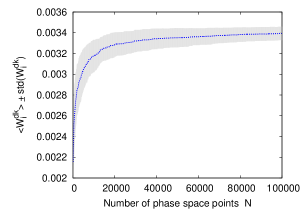
In Figure 1, we illustrate the calibration of the three parameters $N,m$ and $\xi$ based on $pp\rightarrow W$ events. First, the number of phase-space points $N$ is increased until the average of the $W_{i}^{\textrm{dk}}$ is constant with respect to the number of phase-space points (left pane). This identifies the number of phase-space points to be used. Next, the true value of $W^{\textrm{dk}}$ is extracted by considering a very large number of production events. Once this value is known, the prefactor $\xi$ in Eq. (6) can be extracted for a given number $m$ of production events so that the resulting estimate $W_{\textrm{max}}^{\textrm{dk}}$ reproduces the true value $W^{\textrm{dk}}$ (right pane). We take the number of production events $m$ large enough so that the associated value of $\xi$ converges to a constant value. That constant then gives the value of $\xi$, thereby fixing the remaining parameter in our prescription. In the code, we have made the conservative choice $(N=10^{4},\,m=20,\,\xi=4)$.

5 Validation

In order to support phenomenological studies in an optimal way, Monte Carlo generators must show a high level of efficiency, while reflecting as much as possible the accuracy of state-of-the-art calculations. Regarding the efficiency, the approach discussed in this paper has been implemented in the MadGraph5 framework, and hence it can be used for a large class of processes within or beyond the standard model in a complete automated way. Moreover, since the decay of a specific event typically requires only a few evaluations of tree-level matrix elements, generating the decay is in general fast. The efficiency and the flexibility of the tool is at the cost of two approximations inherent to the procedure at work:

1. some finite-width effects may be lost in the distributions of events, as the procedure is built upon the narrow width approximation in the first place,

2. only tree-level matrix-elements are used to calculate the weight associated with a specific decay configuration.

We comment on the validity of these two approximations in this section.

5.1 Finite width effects

Figure 2: Distribution of events with respect to the invariant mass of the muon pair (left pane) and with respect to $\sqrt{\hat{s}}$ (right pane) in $pp\rightarrow\mu^{+}\mu^{-}e^{+}\nu_{e}$ events. The two histograms result from two distinct procedures to generate the events: either MadGraph5 is used to generate $pp\rightarrow ZW^{+}$ (LO accuracy) which are subsequently decayed using MadSpin (solid histogram) or MadGraph5 is used to the generate $pp\rightarrow\mu^{+}\mu^{-}e^{+}\nu_{e}$ in one shot, so that all finite-width effects are systematically included (dashed histogram).

We verified the validity of the first approximation by considering a large class of tree-level processes involving heavy resonances. We generated events in two different ways (a) we used MadGraph5 to generate undecayed events, which were subsequently decayed using MadSpin, (b) we used MadGraph5 to generate decayed events, considering a finite width for the heavy resonances at all stages of the generation (and including also the non-resonant contributions). We compared a large number of distributions involving the transverse momentum, the angular separation, and the invariant mass of the final state particles. We obtained very good agreement between distributions resulting from the generation procedures (a) and (b). Some differences were observed in the tails of resonant invariant mass distributions or close to threshold, as expected.

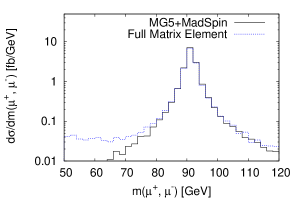
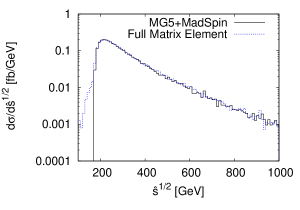
To illustrate the largest observed deviations, let us consider the specific example of diboson production at the LHC in the channel $pp\rightarrow ZW^{+}\rightarrow\mu^{+}\mu^{-}e^{+}\nu_{e}$. Figure 2 shows the distribution of events with respect to the invariant mass of the muon pair (left pane) and with respect to $\sqrt{\hat{s}}$ = the invariant mass of the colliding partons (right pane) resulting from the previously-mentioned procedures to generate events: (a) MadGraph5 is used to generate $pp\rightarrow ZW^{+}$ events (at leading order accuracy) which are subsequently decayed using MadSpin (solid histogram), (b) MadGraph5 is used to the generate $pp\rightarrow\mu^{+}\mu^{-}e^{+}\nu_{e}$ events in one shot (including also the non-resonant diagrams with the photon splitting $\gamma^{*}\rightarrow\mu^{+}\mu^{-}$), so that all finite-width effects are systematically included (dashed histogram). In this last case, we impose the cut $m(\mu^{+},\mu^{-})>40$ GeV.

As expected, procedure (a) fails to reproduce the correct distribution of events far away from the resonance region $m(\mu^{+},\mu^{-})\approx m_{Z}$, as the distribution of events in these regions is sensitive to the non-resonant contributions involving the photon splitting $\gamma^{*}\rightarrow\mu^{+}\mu^{-}$. We observe though that the distribution of events with respect to the invariant mass of the muon pair is accurately reproduced in a rather extended region around the pole mass $m_{Z}$: although the Z boson is generated on its mass shell in undecayed events, off-shell effects are recovered to a very good accuracy when decaying the events. We also observe a good agreement for the distribution of events with respect to the invariant mass of the colliding partons ($\sqrt{\hat{s}}$), except below the threshold region $\sqrt{\hat{s}}\approx m_{Z}+m_{W}$ where the effects from the finite widths of the Z and W bosons are of primary importance and cannot be reproduced in the narrow width approximation. An ad-hoc approach to improve the description below the $m_{Z}+m_{W}$ threshold would be to allow for a (small) change in $\sqrt{\hat{s}}$ when the ratio $(m_{Z}+m_{W})/\sqrt{\hat{s}}$ is close to one. We leave this for future work.

5.2 Spin correlation effects in NLO events

Figure 3: Next-to-leading-order cross sections differential in $\cos\phi$, $\cos(\theta_{+})$ and $p_{T}(l^{+})$ for $pp\rightarrow t\bar{t}$ events in the dileptonic channel. The angles are defined in the text.

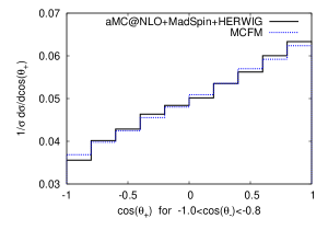
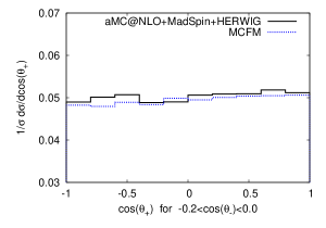
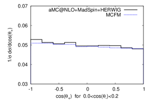
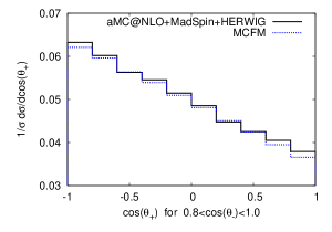
For the decay of Les Houches Events generated at next-to-leading-order accuracy, the procedure in MadSpin retains spin correlation effects at tree-level accuracy, i.e. no information from the virtual amplitude is used in calculating the weight of a specific decay configuration. The validity of this second approximation can be assessed in some specific cases by comparing distributions of events against predictions including spin correlation effects at a higher level of accuracy. One possibility is to generate these predictions with MCFM (provided that it includes the process at work) which includes all QCD corrections when calculating the weight of a decay configuration. A limitation of such a comparison is that MCFM provides only fixed-order predictions, whereas MadSpin is embedded in a scheme involving NLO calculation matched to parton shower. A more advanced validation procedure (e.g. involving NLO predictions in the complex mass scheme matched to parton shower) is beyond the scope of this paper.

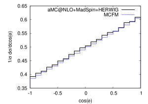
In this section, we present comparison plots with the results from the Monte Carlo program MCFM for $t\bar{t}$ and single-$t$ production at the LHC at $\sqrt{s}=8\mathrm{\,TeV}$. For single-$t$ [21] we used the four-flavor scheme and considered production via the $t$-channel. In both processes the $t$ and $\bar{t}$ decay semi-leptonically (b quark + lepton + neutrino). QCD corrections in the decay itself are ignored. The relevant masses are $m_{t}=172.5\mathrm{\,GeV}$ and $m_{b}=4.75\mathrm{\,GeV}$. Jets are reconstructed by means of the anti-$k_{T}$ algorithm [22], with $R_{\mathrm{cut}}=0.4$ and $(p_{T})_{\mathrm{min}}=25\mathrm{\,GeV}$. For $t\bar{t}$ we have used the first PDF set from MSTW2008nlo68cl (v5.7) [23]. In that case $\alpha_{S}(M_{Z})=0.12018$, which evolves by two-loop running. For single-$t$ we used MSTW2008nlo68cl_nf4 (v5.8.4) instead [24], where $\alpha_{S}(M_{Z})=0.11490$. The renormalization and factorization scales are set equal to the same scale $\mu$. In the case of $t\bar{t}$, $\mu$ is given by the average of the $t$ and $\bar{t}$ transverse masses, while in the case of single-$t$ we use four times the $b$ transverse mass, this choice being based on the work of [25]. In both cases, top quarks are decayed in the semi-leptonic channel. Events are showered and hadronized with the program Herwig [16].

Figure 4: Next-to-leading-order cross sections differential in $\cos(\theta)$ and $p_{T}(l^{+})$ for single-top production in the four flavor scheme (t-channel only). The angle $\theta$ is defined in the text.

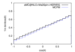
For top quark pair production, the observables that are most sensitive to spin correlation effects were discussed in [26]:

• $\cos(\phi)$, where $\phi$ is the angle between the direction of flight of $l^{+}$ in the $t$ rest frame and the direction of flight of $l^{-}$ in the $\bar{t}$ rest frame,

• $\cos(\theta_{\pm})$, where $\theta_{+}$ ($\theta_{-}$) is the angle between the direction of flight of $l^{+}$ ($l^{-}$) in the $t$ ($\bar{t}$) rest frame and positive beam direction.

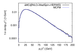
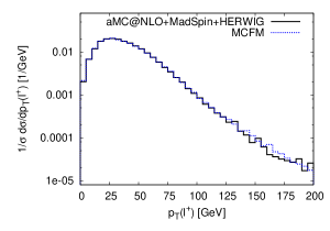
As can be seen in Figure 3, predictions for these observables using the scheme outlined in this paper (aMC@NLO+MadSpin+Herwig) are overall in very good agreement with those generated by MCFM. A good agreement is also found for the $p_{T}$ spectrum of the positively-charged lepton [Figure 3, bottom right].

For single-top production, the observables that are most sensitive to spin correlation effects were discussed in [27]. In the case of t-channel production, the angle $\theta$ is defined in the $t$ rest frame as the angle between the directions of flight of $l^{+}$ and the hardest non-$b$-tagged jet. In this case as well, predictions using the scheme outlined in this paper (aMC@NLO+MadSpin+Herwig) are in good agreement with those generated by MCFM (see Figure 4). The apparent difference in normalization of the two curves in the plot on the left-hand side of Figure 4 is due to the definition of the observable. For the aMC@NLO+MadSpin+Herwig predictions there are slightly more events with a non-$b$-tagged jet compared to the fixed order MCFM results (80% versus 76%, respectively).

6 Application: top-quark pair production in association with a light Higgs boson

In order to illustrate the capabilities of the tool, we apply it to the case of top-quark pair production in association with a light Higgs boson at the LHC (running at 8 TeV), considering both the scalar and pseudo-scalar hypotheses for the Higgs boson. Due to the large irreducible QCD background, any search strategy for this Higgs production process relies strongly on the accuracy of the Monte Carlo predictions. QCD correction to these processes has been analyzed by two groups [11, 13] and a comparison between these independent calculations has appeared in Ref. [28]. In these works it was shown that the NLO corrections are very mild, in particular on shapes of distributions.

To the best of our knowledge, the problem of retaining spin correlation effects in events generated at NLO accuracy has not been addressed yet for these processes. This problem is trivially solved using the scheme proposed in this paper: NLO parton-level events are generated with aMC@NLO, (LHC at 8 TeV, $\textrm{PDF set}=\textrm{MSTW2008(n)lo68cl}$, $m_{H}=m_{A}=125$ GeV, $\mu_{R}=\mu_{F}=(m_{T}(H/A)m_{T}(t)m_{T}(\bar{t}))^{(1/3)}$, no cuts) and then decayed with MadSpin before they are passed to Herwig for shower and hadronization. In this illustration, top and anti-top quarks are decayed semi-leptonically, whereas the Higgs is decayed into a pair of b quarks.

Figure 5: Next-to-leading-order cross sections differential in $p_{T}(l^{+})$ (left pane) and in $\cos\phi$ (right pane) for $t\bar{t}H$ events with or without spin correlation effects. For comparison, also the leading-order results are shown. Events were generated with aMC@NLO, then decayed with MadSpin, and finally passed to Herwig for shower and hadronization.

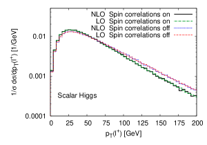
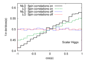
Figure 5 shows the normalized distribution of events with respect to $\cos(\phi)$ (which was defined in the previous section), and with respect to the transverse momentum of the hardest positively-charged lepton. Although spin correlation effects significantly distort the distribution of events with respect to $\cos(\phi)$, their impact on the $p_{T}$ spectrum of the leptons is milder, except at large transverse momentum. The relatively larger effect in the tail of this distribution can easily be understood from the fact that the inclusion of the spin correlations is a unitary procedure: a small change at low $p_{T}$, where the cross section is large, needs to be compensated by a larger (relative) effect at high $p_{T}$.

It is interesting that spin correlations have a much more dramatic influence on the shape of the $p_{T}$ spectrum than NLO corrections: the leading order results fall directly on top of the NLO results for these normalized distributions (both without spin correlations), as it can be seen by comparing the dotted blue and dash-dotted red curves. This suggests that preserving spin correlations is more important than including NLO corrections for this observable. However, we observe that the inclusion of both, as it is done here, is necessary for an accurate prediction of the distribution of events with respect to $\cos(\phi)$. In general, a scheme including both spin correlation effects and QCD corrections is preferred: it retains the good features of a NLO calculation, i.e. reduced uncertainties due to scale dependence (not shown), while keeping the correlations between the top decay products.

Figure 6: Next-to-leading-order cross sections differential in $p_{T}(l^{+})$ (left pane) and in $\cos\phi$ (right pane) for $t\bar{t}A$ events with or without spin correlation effects. Events were generated with aMC@NLO, then decayed with MadSpin, and finally passed to Herwig for shower and hadronization.

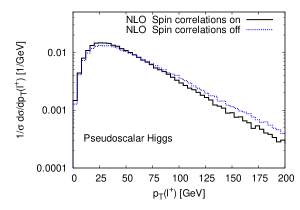
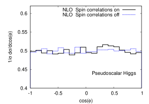
The results for the pseudo-scalar Higgs boson are shown in Figure 6. The effects of the spin correlations on the transverse momentum of the charged lepton are similar as in the case of a scalar Higgs boson: about 10% at small $p_{T}$, increasing to about 40% at $p_{T}=200$ GeV. On the other hand, the $\cos(\phi)$ does not show any significant effect from the spin-correlations. Therefore this observable could possibly help in determining the CP nature of the Higgs boson, underlining the importance of the inclusion of the spin correlation effects.

7 Conclusion

In this paper, we discussed the decay of events in a LHE file. We showed that the decay can be treated in a completely generic way in the MadGraph5 framework. The procedure is particularly efficient to generate unweighted decayed events, while preserving spin correlation effects at tree-level accuracy. Some features associated with the finite width of the resonances to be decayed are also successfully reproduced. The practical implementation of this procedure –dubbed MadSpin– makes use of the user-friendly MadGraph5 interface, so that it can be trivially applied to a very large category of processes. As an illustration we applied the tool to the case of top quark pair production in association with a Higgs boson at the LHC, and showed for the first time predictions at next-to-leading order including spin correlation effects in the angular distributions of the leptons.

Limitations of the approach are inherent to restrictions on the validity of the narrow width approximation. As an example, distributions of events very close to threshold are sensitive to finite width effects, and cannot be predicted accurately within the procedure discussed in this paper. Practical limitations are also expected depending on the complexity of the process at work. In particular, the unweighting procedure in MadSpin has not been optimized for decay chains which cannot be split into a sequence of two-body decays. This could be improved by boosting the efficiency of the unweighting procedure with the use of adaptive Monte Carlo techniques.

Within the range of validity of the method, MadSpin gives access to a large set of applications. In particular, it should be stressed that the algorithm also applies to any BSM decay chain processes that can be handled in the narrow width approximation. The most obvious benefit of this work is that MadSpin provides a very convenient way to decay events generated at next-to-leading-order accuracy, as it is naturally embedded in a Monte Carlo scheme. Although only tree-level matrix elements are used to unweight the decay configurations, we have shown for specific processes that this procedure captures essentially all spin correlation effects as predicted by a full next-to-leading-order calculation. A systematic study of the level of accuracy delivered by this procedure for generic processes is beyond the scope of this paper. Nevertheless, a plausible assumption is that information from one-loop corrections in the production process are irrelevant as far as spin correlations are concerned. Therefore MadSpin –in combination with a next-to-leading-order Monte Carlo generator– is expected to give access to event generation with an improved accuracy in many instances.

Appendix A Manual

The MadSpin program is part of the MadGraph5 distribution from version 2.0.0 onwards. As a consequence, the MadGraph5 website can be used for downloading the code but also to submit questions or report bugs. The code can either be used in standalone mode or called by another program of the MadGraph5 Suite (i.e. MadEvent or aMC@NLO). In standalone, one launches a MadSpin session by typing:

./MadSpin/madspin

This opens a prompt, similar to that of the MadGraph5 Suite. The following commands are then available:

• import FILE: imports the LO or NLO lhe file and reads the associated header in order to load relevant information, e.g. the relevant model.

• define LABEL = PART1 PART2 … : allows to define an additional multi-particle tag. The multi-particle tags defined in the header of the file are automatically recognized.

• decay PROCESS: specifies the decay branch initiated by an unstable particle to be decayed by MadSpin. Multi-particle tags can be used for the final state particles.

• set OPTION VALUE: allows to change some internal options of MadSpin such as the seed or the value of the maximal weight in the unweighting procedure. Type “help options” in the interface for more details on the various available options.

• launch: runs MadSpin according to the specified options/decay channels.

• help COMMAND: provides detailed information on a specific command.

As stated above, MadSpin can also be called directly via the MadEvent/aMC@NLO script (via the launch command or the ./bin/generate_events script). In this case, the script will request some information about the programs to run. The exact question depends on the programs installed on your computer and on the QCD order of the process (LO or NLO), but it typically looks like this:

Which programs do you want to run?
  0 / auto    : running existing card
  1 / parton  :  Madevent
  2 / pythia  : MadEvent + Pythia.
  3 / pgs     : MadEvent + Pythia + PGS.
+10 / +madspin: adding MadSpin to the run (before running Pythia)
[0, auto, 1, parton, 11, parton+madspin, 2, pythia, 12, ... ]

If you choose to run MadSpin (i.e. if you enter one of the following answers: 11, 12, 13, parton+madspin, pythia+madspin, pgs+madspin), the program will propose, in a second step, to edit the madspin_card.dat. This file contains the command lines associated with the MadSpin program that we just described. Note that MadGraph5 will figure out which event file has to be decayed, so that you do not need to include the “import” command in this file. After these questions have been answered, MadGraph5 proceeds with the Monte Carlo generation: (1) it generates the LHE event file before decay, (2) it executes MadSpin and (3) if requested, it submits the decayed events to a shower/hadronisation program.

References

- [1] J. M. Campbell, R. K. Ellis and F. Tramontano, Phys. Rev. D 70, 094012 (2004) [hep-ph/0408158].
- [2] J. M. Campbell and F. Tramontano, Nucl. Phys. B 726, 109 (2005) [hep-ph/0506289].
- [3] S. Badger, J. M. Campbell and R. K. Ellis, JHEP 1103, 027 (2011) [arXiv:1011.6647 [hep-ph]].
- [4] P. Richardson, JHEP 0111, 029 (2001) [hep-ph/0110108].
- [5] P. Meade and M. Reece, hep-ph/0703031.
- [6] S. Frixione, E. Laenen, P. Motylinski and B. R. Webber, JHEP 0704, 081 (2007) [hep-ph/0702198 [HEP-PH]].
- [7] S. Frixione and B. R. Webber, JHEP 0206, 029 (2002) [hep-ph/0204244].
- [8] S. Frixione, E. Laenen, P. Motylinski and B. R. Webber, JHEP 0603, 092 (2006) [hep-ph/0512250].
- [9] S. Frixione, P. Nason and G. Ridolfi, JHEP 0709, 126 (2007) [arXiv:0707.3088 [hep-ph]].
- [10] S. Alioli, P. Nason, C. Oleari and E. Re, JHEP 1006 (2010) 043 [arXiv:1002.2581 [hep-ph]].
- [11] R. Frederix, S. Frixione, V. Hirschi, F. Maltoni, R. Pittau and P. Torrielli, Phys. Lett. B 701, 427 (2011) [arXiv:1104.5613 [hep-ph]].
- [12] S. Hoeche, F. Krauss, M. Schonherr and F. Siegert, arXiv:1111.1220 [hep-ph].
- [13] M. V. Garzelli, A. Kardos, C. G. Papadopoulos and Z. Trocsanyi, Europhys. Lett. 96 (2011) 11001 [arXiv:1108.0387 [hep-ph]].
- [14] T. Sjostrand, S. Mrenna and P. Z. Skands, JHEP 0605, 026 (2006) [hep-ph/0603175].
- [15] T. Sjostrand, S. Mrenna and P. Z. Skands, Comput. Phys. Commun. 178, 852 (2008) [arXiv:0710.3820 [hep-ph]].
- [16] G. Corcella, I. G. Knowles, G. Marchesini, S. Moretti, K. Odagiri, P. Richardson, M. H. Seymour and B. R. Webber, JHEP 0101, 010 (2001) [hep-ph/0011363].
- [17] J. Alwall, M. Herquet, F. Maltoni, O. Mattelaer and T. Stelzer, JHEP 1106, 128 (2011) [arXiv:1106.0522 [hep-ph]].
- [18] C. Degrande, C. Duhr, B. Fuks, D. Grellscheid, O. Mattelaer and T. Reiter, Comput. Phys. Commun. 183, 1201 (2012) [arXiv:1108.2040 [hep-ph]].
- [19] P. de Aquino, W. Link, F. Maltoni, O. Mattelaer and T. Stelzer, Comput. Phys. Commun. 183, 2254 (2012) [arXiv:1108.2041 [hep-ph]].
- [20] F. Maltoni and T. Stelzer, JHEP 0302, 027 (2003) [hep-ph/0208156].
- [21] J. M. Campbell, R. Frederix, F. Maltoni and F. Tramontano, Phys. Rev. Lett. 102, 182003 (2009) [arXiv:0903.0005 [hep-ph]].
- [22] M. Cacciari, G. P. Salam and G. Soyez, JHEP 0804, 063 (2008) [arXiv:0802.1189 [hep-ph]].
- [23] A. D. Martin, W. J. Stirling, R. S. Thorne and G. Watt, Eur. Phys. J. C 63, 189 (2009) [arXiv:0901.0002 [hep-ph]].
- [24] A. D. Martin, W. J. Stirling, R. S. Thorne and G. Watt, Eur. Phys. J. C 70, 51 (2010) [arXiv:1007.2624 [hep-ph]].
- [25] R. Frederix, E. Re and P. Torrielli, JHEP 1209, 130 (2012) [arXiv:1207.5391 [hep-ph]].
- [26] W. Bernreuther, A. Brandenburg, Z. G. Si and P. Uwer, Nucl. Phys. B 690, 81 (2004) [hep-ph/0403035].
- [27] G. Mahlon and S. J. Parke, Phys. Rev. D 55, 7249 (1997) [hep-ph/9611367].
- [28] S. Dittmaier, S. Dittmaier, C. Mariotti, G. Passarino, R. Tanaka, S. Alekhin, J. Alwall and E. A. Bagnaschi et al., arXiv:1201.3084 [hep-ph].