Can we measure the slopes of density profiles in dwarf spheroidal galaxies?

Abstract

Using collisionless $N$-body simulations of dwarf galaxies orbiting the Milky Way we construct realistic models of dwarf spheroidal (dSph) galaxies of the Local Group. The dwarfs are initially composed of stellar disks embedded in dark matter haloes with different inner density slopes and are placed on an eccentric orbit typical for Milky Way subhaloes. After a few Gyr of evolution the stellar component is triaxial as a result of bar instability induced by tidal forces. Observing the simulated dwarfs along the three principal axes of the stellar component we create mock data sets and determine the corresponding half-light radii and line-of-sight velocity dispersions. Using the estimator proposed by Wolf et al. we calculate the masses within half-light radii. The masses obtained in this way are over(under)estimated by up to a factor of two when the line of sight is along the longest (shortest) axis of the stellar component. We then divide the initial stellar distribution into an inner and outer population and trace their evolution in time. The two populations, although strongly affected by tidal forces, retain different density profiles even after a few Gyr of evolution. We measure the half-light radii and velocity dispersions of the stars in the two populations along different lines of sight and use them to estimate the slope of the mass distribution in the dwarf galaxies following the method recently proposed by Walker & Peñarrubia. The inferred slopes are systematically over- or underestimated, depending on the line of sight. In particular, when the dwarf is seen along the longest axis of the stellar component, a significantly shallower density profile is inferred than the real one measured from the simulations. Given that most dSph galaxies in the Local Group are non-spherical in appearance and their orientation with respect to our line of sight is unknown, but most probably random, the method can be reliably applied only to a large sample of dwarfs when these systematic errors are expected to be diminished.

1 Introduction

One of the key predictions of theories of structure formation based on cold dark matter is that the dark matter haloes should possess cuspy density profiles in the centre of bound structures such as galaxies and galaxy clusters (Navarro, Frenk & White 1997, hereafter NFW). The prediction, obtained via the use of $N$-body simulations of gravitational instability of dark matter only, relied on the assumption that baryons play relatively minor role in shaping the final density structure of bound objects. Comparison of this prediction to observations of low surface brightness galaxies resulted in strong disagreement, as modelling of rotation curves of such objects consistently pointed towards preference for cored, rather than cuspy dark matter density profiles required by the data (e.g. de Blok, McGaugh & Rubin 2001). The tension came to be known as the cusp/core problem.

A number of solutions to the problem has been proposed over the years including the possibility that the difficulties associated with modelling of the data prevent us from detecting the cusps which really are there and the proposals to modify the properties of dark matter postulating that it may be self-interacting (Spergel & Steinhardt 2000; Vogelsberger, Zavala & Loeb 2012). The most effective approach, however, turned out to be the one questioning the aforementioned assumption of baryon physics playing little or no role in shaping dark matter haloes. This approach has recently led to more detailed modelling of star-formation related processes using $N$-body and hydro simulations in the cosmological context and succeeded in producing disky dwarf galaxies with shallower inner dark matter density slopes (Governato et al. 2010). The success of this work relied on including all the crucial baryonic processes like gas cooling, star formation, cosmic UV background heating and gas outflows driven by supernovae but the critical improvement involved resolving individual star-forming regions and allowing only high density gas clouds to form stars. The predictions of this theoretical work were successfully compared to the properties of late-type dwarf galaxies from the THINGS survey (Oh et al. 2011).

The question remains, if similar agreement can be reached for early-type galaxies, in particular dwarf spheroidals (dSph) available for observation in the immediate vicinity of the Milky Way. In systems supported by random rather than rotational motions, an additional complication in the modelling occurs due to the fact that such systems may be characterized by a variety of velocity anisotropy profiles a priori unknown which leads to the degeneracy between the model parameters. The inferences concerning dark matter distribution in dSph galaxies are usually made based on solving the lowest-order Jeans equation that relates the mass distribution to observables such as the density distribution of the stars and their velocity dispersion profile. Solving for the underlying mass distribution requires however strong assumptions concerning the anisotropy of stellar orbits.

This degeneracy can be partially lifted by including higher-order Jeans equations and modelling also the fourth velocity moment which is sensitive mainly to velocity anisotropy (Łokas 2002). This strategy works if the dark matter profile is parametrized only by the virial (or total) mass and concentration (or equivalently scale-length) and has been successfully applied to the Draco dSph galaxy (Łokas, Mamon & Prada 2005). However, if the inner dark matter slope is additionally considered as a free parameter, another degeneracy occurs, this time between the inner slope and concentration, and equally good fits to the velocity moments can be obtained for cuspy and cored dark matter profiles (Łokas & Mamon 2003; Sánchez-Conde et al. 2007).

With the large kinematic samples currently available for some of the classic dSph galaxies of the Local Group it has recently become possible to model their dark matter distribution using different approaches based on orbit superposition and/or working with the distribution function itself and modelling of discrete data rather than velocity moments which require binning of the data and thus lead to loss of information (Chanamé, Kleyna & van der Marel 2008; Jardel & Gebhardt 2012; Breddels et al. 2012). The conclusions from this approach are far from consensus and seem to depend on the object studied and the details of the method used. For example Breddels et al. cannot firmly distinguish between a core and a cusp in the Sculptor dSph while Jardel & Gebhardt claim to find preference for a core-like dark matter distribution in Fornax. The subject thus requires further study and different approaches, one promising example being the use of the motions of globular clusters in dSph galaxies (see Goerdt et al. 2006 and Cole et al. 2012 for an application of this method to the Fornax dwarf).

An interesting and particularly simple method to measure the slope of density profile in dSph galaxies has been recently proposed by Walker & Peñarrubia (2011, hereafter WP11). The method relies on the use of separate stellar populations identified in a dSph by their different metallicity and simple mass estimators measuring the mass within half-light radii of each population from these radii and their respective velocity dispersions. Since both populations are expected to be in equilibrium in the global gravitational potential of the dwarf, the two mass measurements at two different scales lead to a direct measurement of the mass slope which can be translated to a constraint on the inner density slope. The application of this method to the Fornax and Sculptor dSph galaxies led WP11 to the conclusion that both possess dark matter density profiles significantly shallower than the cuspy profiles predicted by NFW.

In this work we test the method of WP11 using realistic models of dSph galaxies formed in $N$-body simulations of tidal stirring of disky dwarfs embedded in dark matter haloes of different inner slopes in the gravitational field of the Milky Way. The tidal stirring scenario for the formation of dSph galaxies, originally proposed by Mayer et al. (2001), has been demonstrated to reproduce well the basic properties of the population of dSph galaxies in the Local Group (Mayer et al. 2007; Klimentowski et al. 2009a; Kazantzidis et al. 2011; Łokas, Kazantzidis & Mayer 2011). Although WP11 tested their approach using $N$-body realizations of dwarf galaxies, they only used spherical models and concluded that any systematic errors can lead to the underestimation of the mass slope and thus dwarfs cannot appear more core-like than they really are.

However, dSph galaxies of the Local Group are known to be non-spherical, with an average ellipticity of 0.3 (Mateo 1998; Łokas et al. 2011, 2012a). We expect this fact to have important consequences for the mass and mass slope estimates. As already discussed by Łokas et al. (2010a), when the dwarfs are observed along the longest (shortest) axis of the stellar component, their mass is significantly over(under)estimated even if modelling of the velocity anisotropy is included in the analysis. The non-sphericity may affect simple mass estimators used in the method of WP11 even more and thus bias the inferred mass slope estimates. In the simulations of tidal stirring of dwarf galaxies we use here non-spherical, triaxial stellar components form naturally as a result of bar instability induced by tidal forces from the Milky Way and thus such models are suitable for testing the effects of non-sphericity on mass and mass slope estimates.

The paper is organized as follows. In section 2 we describe the simulations used in this work and characterize the main properties of the simulated dwarfs used for the further analysis. Section 3 is devoted to the problem of mass estimation; we present the observables used, estimate the masses within half-light radii and compare them to real masses measured directly from the simulations. In section 4 we describe the evolution of properties of two stellar populations selected from the stellar component of the dwarfs and in section 5 we use them to estimate the slope of the density profile in the simulated dwarfs. The discussion of the results follows in section 6.

2 The simulated dwarfs

In this work we used a subset of simulations described in more detail in Łokas, Kazantzidis & Mayer (2012b). The dwarf galaxy models consisted of exponential stellar disks embedded in spherical dark matter haloes with density profiles of the form

$$\rho(r)=\frac{\rho_{\rm char}}{(r/r_{\rm s})^{\alpha}\,(1+r/r_{\rm s})^{3-\alpha}}.$$ (1)

Such profiles are characterized by an asymptotic inner slope $r^{-\alpha}$, which we allow to vary, and an outer slope $r^{-3}$ which is kept fixed. The detailed properties of density profiles given by formula (1) are discussed in Łokas (2002) and Łokas & Mamon (2003) who applied them in dynamical modelling of dSph galaxies and the Coma cluster. All our dwarf galaxies have the same virial mass of $M_{\rm vir}=10^{9}M_{\odot}$ and concentration parameter $c=r_{\rm vir}/r_{\rm s}=20$, but different $\alpha$, which requires slightly different values of the characteristic density $\rho_{\rm char}$ in equation (1). We consider $\alpha=1$ (which corresponds to the NFW profile), and two shallower inner slopes, a mild cusp with $\alpha=0.6$ and an almost cored profile with $\alpha=0.2$.

The dark matter haloes were populated with stellar disks of mass equal to $m_{\rm d}=0.02M_{\rm vir}$. The disk scale lengths were $R_{\rm d}=0.41$ kpc in the radial direction (corresponding to a dimensionless spin parameter of $\lambda=0.04$, following Mo, Mao & White 1998), and $z_{\rm d}=0.2R_{\rm d}$ in the vertical direction. Each numerical realization of the dwarf galaxy contained $N_{\rm h}=10^{6}$ dark matter and $N_{\rm d}=5\times 10^{5}$ disk particles and the adopted gravitational softenings were $\epsilon_{\rm h}=60$ pc and $\epsilon_{\rm d}=20$ pc, respectively.

Figure 1: The slope of the dark matter density profile of the haloes of the initial dwarf models as a function of radius. Symbols show the values measured from the $N$-body realizations by fitting a power-law, while the lines correspond to the values calculated from the analytic formula of equation (1).

It is worth emphasizing that the $\alpha$ denotes the limiting inner slope and thus differs from the real slope one actually measures at any radius $r>0$. To illustrate this, in Figure 1 we plot the dark matter density slope $-\gamma={\rm d}\log\rho/{\rm d}\log r$ as a function of radius. The solid, dashed and dotted lines show respectively the slope derived directly from formula (1). The symbols, on the other hand, show the corresponding values of the slope measured from the numerical realizations of the haloes by fitting a straight line to data points of $\log\rho(\log r)$. The latter measurements extend down to radii of the order of 3 dark matter softening scales, i.e. about 0.2 kpc. The two measurements agree except for small variations inherent in the numerical realizations.

At 0.2 kpc, and any larger radius, the actual slope is significantly lower than the limiting value $-\alpha$. In particular, at $r=0.5$ kpc the dark matter density slopes of our dwarfs are initially in the range $(-1.6,-1)$ (see Figure 1) and thus similar to those predicted by the recent simulations of Governato et al. (2012) for dwarfs of stellar masses of the order of $2\times 10^{7}$ M_⊙ at redshift $z=0$. Given that the inner slopes of dark matter haloes are not significantly altered after redshift of about $z=1$ (Governato et al. 2010) we thus conclude that our assumed dark matter profiles are consistent with the latest findings concerning the properties of dwarfs formed in cosmological simulations where star formation processes are sufficiently resolved. Our progenitor dwarfs can therefore be considered as idealized versions of such dwarfs which we assume were accreted by a Milky Way-like host at about $z=1-2$.

The dwarf galaxies were placed on an orbit (at apocentre) around a primary galaxy with the present-day structural properties of the Milky Way (Widrow & Dubinski 2005; Kazantzidis et al. 2011) and their evolution was followed for 10 Gyr using the $N$-body code PKDGRAV (Stadel 2001). The dwarf galaxy disk was oriented so that its internal angular momentum was inclined to the orbital angular momentum by $i=45^{\circ}$. Out of five orbits of different size and eccentricity considered in Łokas et al. (2012b) we choose only one, namely R1, with orbital apocentre $r_{\rm apo}=125$ kpc and pericentre $r_{\rm peri}=25$ kpc. This choice was motivated by the fact that only for this orbit for all values of $\alpha$ at some stage of the evolution a dSph galaxy is formed and it survives for long enough to provide sufficient number of models as input for the present analysis. We also note that this is a typical orbit of a satellite accreted by a Milky Way-like galaxy at redshift $z=1-2$ (Diemand et al. 2007; Klimentowski et al. 2010).

Figure 2: The evolution of the slope of the density profile of different components in time measured at the radius $r=0.2$ (left panels) and $r=0.5$ kpc (right panels) from the centre of the dwarf. The rows from top to bottom give results for dark matter, stars and the two components combined. The solid, dashed and dotted lines show slopes measured for dwarfs with haloes of different initial inner slope $\alpha=1,0.6$ and 0.2, respectively. Thin vertical lines indicate pericentre passages.

Let us first consider the evolution of the slope of the density profile of different components in time, as the dwarfs orbit the Milky Way, since this is the primary focus of this work. Figure 2 shows how the local slope of density profile of dark matter, stars and the two components combined (from the top to the bottom row) changes due to tidal effects. In the two columns we plot the slopes measured at two scales, $r=0.2$ (left panels) and $r=0.5$ kpc (right panels) which bracket the scales where the measurements from the kinematic data can be performed since these are of the order of the half-light radii of our simulated dwarf galaxies at later stages of evolution. Note that we do not consider here the limiting slope of the dark matter density profile at $r\rightarrow 0$, as was done e.g. by Kazantzidis et al. (2004), but we measure the slope at a fixed, non-zero radius.

Figure 3: The evolution of different properties of the dwarf galaxy in time. The panels from top to bottom plot the luminosity, mass (of stars and dark matter), axis ratios, the ratio of the rotation velocity to the velocity dispersion $V/\sigma$ and the anisotropy parameter $\beta$ of the stellar component. All quantities were measured within radius $r<0.5$ kpc. In each panel the solid, dashed and dotted lines show the results for dwarfs embedded in dark matter haloes with different initial inner slope $\alpha=1,0.6$ and 0.2, respectively. Thin vertical lines indicate pericentre passages.

The results demonstrate that in the case of dark matter the slopes evolve towards stepper ones with time which reflects the overall steepening of the profiles due to tidal stripping. In addition, the hierarchy of values of the slopes for different $\alpha$ is preserved, i.e. the local slopes are always higher for $\alpha=0.2$ than for $\alpha=1$, except for the later stages when the slope at $r=0.5$ kpc for the $\alpha=0.2$ case varies strongly with time. This occurs when this dwarf galaxy starts to dissolve before it is completely destroyed at about $t=8$ Gyr, which is why we do not show results beyond that time for this case in Figure 2 and any of the following plots.

In the case of the stellar component the interpretation of the evolution of the slope is less straightforward because of the bar formation after the first pericentre passage. However, at $r=0.5$ kpc the stellar density profile also steepens due to mass loss. In the inner region, at $r=0.2$ kpc, the slope remains roughly constant in time and in the case of $\alpha=0.2$ even becomes shallower. In general, at a given scale the dark matter density profile is shallower than the stellar one in the first stages of evolution, reflecting the initial conditions, while the two profiles follow each other at the later stages.

The evolution of other properties of the dwarf galaxies with different $\alpha$ on our chosen orbit is illustrated in Figure 3 (see Kazantzidis, Łokas & Mayer 2013 for a more thorough discussion for different orbits). All quantities shown in the Figure were measured for particles inside $r<0.5$ kpc, which again is motivated by the scale of maximum half-light radii at which the following analysis will be performed. The two upper panels of the Figure illustrate the mass loss the dwarfs suffer, both in terms of stellar content (first panel) and the total mass of stars and dark matter within $r<0.5$ kpc (second panel). To convert the mass of stars to the luminosity we assumed the stellar mass-to-light ratio of 2.5 M_⊙/L_⊙ as is appropriate for an old, single-starburst stellar population typically hosted by dSph galaxies (Bruzual & Charlot 2003). As is immediately seen from the two panels, the mass is more effectively stripped for lower $\alpha$ as the stars and dark matter are more weakly bound in these haloes (see the discussion in Łokas et al. 2012b). In the case of $\alpha=0.2$ after the fourth pericentre, at about $t=8$ Gyr, the dwarf dissolves completely and forms an elongated stream of uniform stellar density. Both $\alpha=0.6$ and $\alpha=1$ dwarfs survive until the end of the simulation with final properties akin to the classical dSph galaxies of the Local Group. In particular, none of those would qualify as an ultra-faint dwarf as is the case for tighter orbits and $\alpha=0.6$ (see Łokas et al. 2012b).

The evolution of the shape of the stellar component of the dwarfs is illustrated in the third and fourth panel of Figure 3 where we plot the axis ratio $b/a$ and $c/a$ where $a,b$ and $c$ are the longest, intermediate and shortest axis determined using the inertia tensor for stars within $r<0.5$ kpc. All dwarfs experience qualitatively the same evolution of the shape: after the first pericentre passage a triaxial shape (or a bar) is formed which becomes more and more spherical in time. The transition towards the spherical shape happens marginally faster for $\alpha=0.2$, especially in terms of $c/a$. The last two panels of Figure 3 illustrate the evolution of the kinematics. The ratio $V/\sigma$ measures the amount of ordered versus random motion: $V$ is the mean rotation velocity around the shortest axis, while $\sigma$ is the 1D velocity dispersion obtained by averaging the dispersion measured along three spherical coordinates. The anisotropy parameter $\beta$ is calculated in the standard way and includes rotation in the second velocity moment around the shortest axis.

The evolution of the shape and kinematics shown in Figure 3 illustrates the transition from the initial disks to dSph galaxies. It is customary to assume that a dSph galaxy is formed when the amount of rotation is sufficiently diminished below some threshold (typically $V/\sigma<1$), and the shape is sufficiently close to spherical (for example $b/a>0.5$ and $c/a>0.5$). Due to different initial properties our dwarfs have different $V/\sigma$ values at the beginning when measured at a fixed radius. In particular at $r=0.5$ kpc the $\alpha=0.2$ has the lowest $V/\sigma<1$ in spite of having a disk because the rotation curve rises slowly with radius as there is less mass in the centre than for other $\alpha$ values. We thus modify the criterion and assume that the dSph galaxy is formed when $V/\sigma$ drops below half of the initial value. For the shape criterion we adopt as usual the threshold of both $b/a$ and $c/a$ greater than 0.5.

3 Estimating masses

Using these criteria for the formation of dSph galaxies we selected 50 outputs (in the time range $t=7.5-10$ Gyr) for $\alpha=1$, 91 outputs ($t=5.5-10$ Gyr) for $\alpha=0.6$ and 22 outputs ($t=4.1-5.1$ Gyr) for $\alpha=0.2$ from the total of 201 outputs saved for each simulation. In the case of $\alpha=0.2$ there are actually more outputs satisfying the criteria, but since after the third pericentre passage the dwarf is strongly perturbed and may departure from equilibrium (as suggested by the strongly varying slope of the density profile in Figure 2) we restrict the sample to earlier outputs as specified above.

For each selected output the dwarf was rotated so that the $x$ axis was oriented along the major, the $y$ axis along the intermediate, and the $z$ axis along the shortest axis of the stellar component. The dwarf galaxy was then “observed”, as a distant observer at infinity would do, along these three axes and mock data sets including the stellar positions and velocities were created for each line of sight. The stellar positions were binned in projected radius $R$ to measure the number density profile. We used bins equally spaced in $\log R$ and to each such profile we fitted the projected Plummer distribution

$$\Sigma(R)=\frac{R_{\rm h}^{2}N}{\pi(R^{2}+R_{\rm h}^{2})^{2}},$$ (2)

adjusting the projected half-light radius $R_{\rm h}$ and normalization $N$. Examples of the measured and fitted profiles (for one output for each $\alpha$) are shown in Figure 6 as triangles and solid lines, respectively. The values of $R_{\rm h}$ for all selected outputs for different $\alpha$ are plotted as a function of time in Figure 7 as solid lines.

We then measured the line-of-sight velocity dispersion $\sigma_{\rm los}$ within $R_{\rm h}$ applying in each case a $3\sigma$ clipping procedure to remove interloper stars until convergence was reached and no more stars were removed from the sample. Note that within $R_{\rm h}$ the contamination from the tidal tails in the immediate vicinity of the dwarf is expected to be very low (Klimentowski et al. 2007, 2009b) and therefore the procedure removes mostly stars with velocities very different from the mean velocity of the dwarf, belonging to tidal debris stripped much earlier. The values of $\sigma_{\rm los}$ measured in this way are plotted as solid lines as a function of time in Figure 8 for different $\alpha$ and different lines of sight.

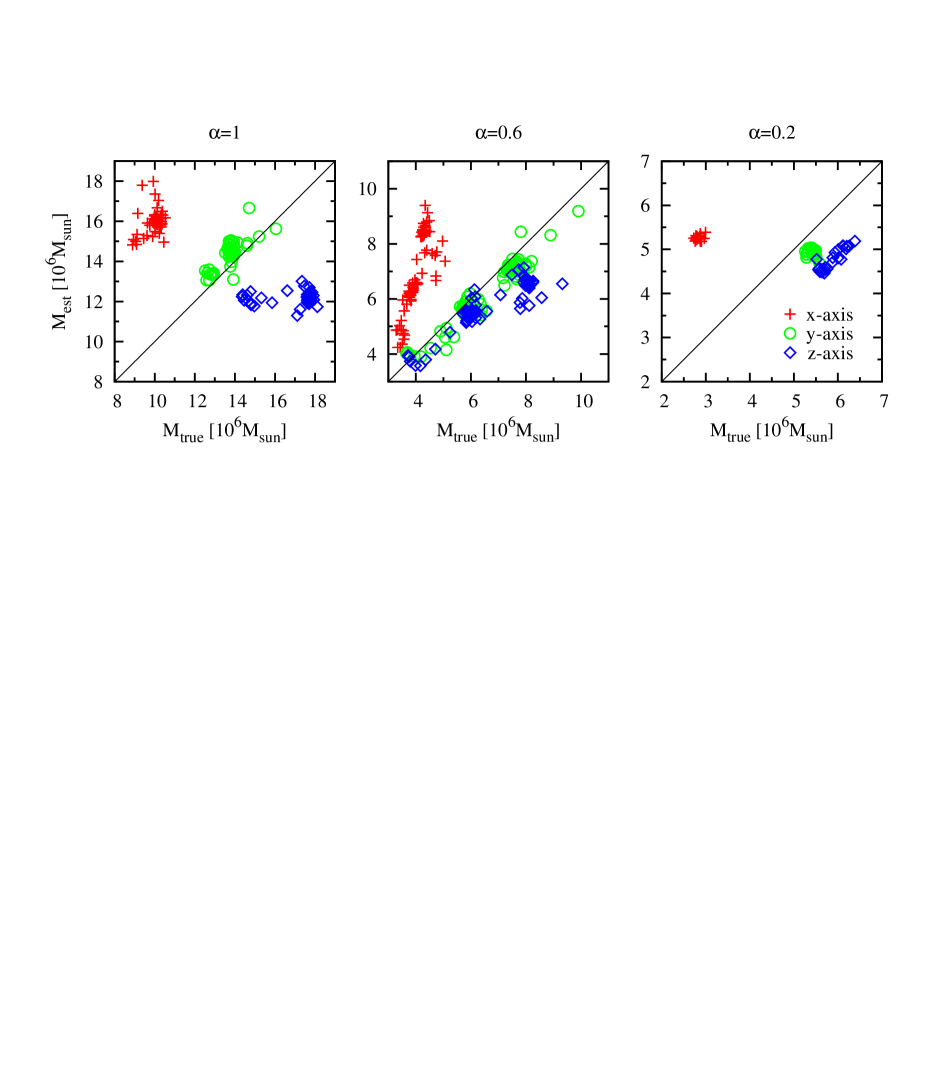
Figure 4: Comparison between the masses $M_{\rm est}$ obtained using estimator (3) and by direct measurement in the simulation $M_{\rm true}$. The three panels from the left to the right show results for $\alpha=1,0.6$ and 0.2, respectively, and the diagonal line in each panel corresponds to the equality of the masses. Symbols of different shape and colour (red crosses, green circles and blue squares) indicate respectively observations performed along different lines of sight: $x$ (longest axis of the stellar component), $y$ (intermediate axis) and $z$ (shortest axis). For each line of sight the half-light radius $R_{\rm h}$ and velocity dispersion $\sigma_{\rm los}$ within $R_{\rm h}$ were calculated using all stars in the appropriate region.

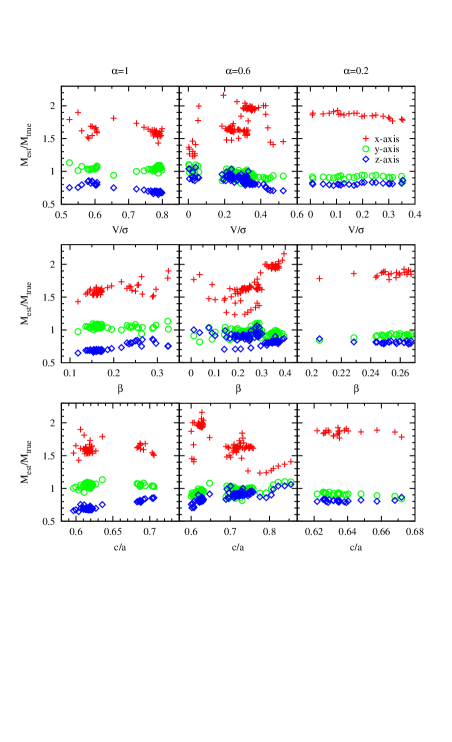
Figure 5: The ratio of the estimated to true mass for all stars as a function of the amount of rotation $V/\sigma$ (upper row), the anisotropy parameter $\beta$ (middle row) and shape in terms of the ratio of the shortest to longest axis of the stellar component $c/a$ (lower row). The columns from the left to the right show results for $\alpha=1,0.6$ and 0.2, respectively. Symbols of different shape and colour indicate observations performed along different lines of sight: $x$ (longest axis of the stellar component), $y$ (intermediate axis) and $z$ (shortest axis).

Using these measurements we estimated the masses of the dwarf galaxies in each output using the formula proposed by Wolf et al. (2010)

$$M_{\rm est}(r_{3})=3\ G^{-1}\sigma_{\rm los}^{2}r_{3}=3.7\ G^{-1}\sigma_{\rm los}^{2}R_{\rm h},$$ (3)

where $r_{3}$ is the radius of the order of the 3D half-light radius found to give results least dependent on anisotropy. For the Plummer profile we use here $r_{3}$ is related to the 3D half-light radius $r_{\rm h}$ and the 2D projected half-light radius $R_{\rm h}$ by $r_{3}/r_{\rm h}=0.94$ and $r_{\rm h}/R_{\rm h}=1.305$, so $r_{3}=fR_{\rm h}$ where $f=1.23$ (see the Appendix of Wolf et al. 2010). The values of the mass estimated in this way were then compared to the real masses contained within $fR_{\rm h}$ in the simulated dwarfs; we will refer to those masses as $M_{\rm true}$.

The values of $M_{\rm est}$ versus $M_{\rm true}$ are plotted in Figure 4. The three panels show the results for all outputs selected for $\alpha=1,0.6$ and 0.2. We clearly see that while for the observations along the intermediate $y$ axis of the stellar component (green circles) the estimated masses are quite close to the corresponding true values, for observations along the longest axis $x$ the masses calculated from formula (3) are overestimated and for observations along the shortest axis $z$ they are underestimated. Only for the observation along the intermediate axis $y$ the agreement between $M_{\rm est}$ and $M_{\rm true}$ is good. The mean and dispersion values of $M_{\rm est}/M_{\rm true}$ are listed in Table 1 in the first row for each $\alpha$. The average numbers show that the masses can be systematically overestimated by up to almost a factor of 2 for the observation along the $x$ axis and underestimated by up to 30 percent for the observation along $z$.

The reason for this systematic bias can be traced to the dependence of the estimates of $R_{\rm h}$ and $\sigma_{\rm los}$ on the line of sight. As shown in Figures 7 and 8, when going from the line of sight along the $x$ axis to the $y$ and $z$ axis, the estimated half-light radius increases, while the velocity dispersion decreases. As the mass estimator (3) depends on the combination $\sigma_{\rm los}^{2}R_{\rm h}$, the direction of the bias is not a priori obvious. It turns out however, that the effect is dominated by the input from the velocity dispersion since it is largest for the line of sight along the longest ($x$) axis and the mass is overestimated in this case.

Figure 6: Examples of measured surface density profiles of stars (symbols) and the corresponding fits of the projected Plummer distribution (2). The three panels from the left to the right show results for a single simulation output in runs with $\alpha=1,0.6$ and 0.2, respectively. In each case the measurements were done along the $y$ axis of the stellar component and at times $t=9.7$, 8.95 and 4.9 Gyr, for $\alpha=1,0.6$ and 0.2, respectively. The fitted values of the half-light radii for the two populations and for all stars are listed in the left corner of each panel.

In Figure 5 we explore how the bias depends on three properties of the dwarfs, namely the amount of rotation $V/\sigma$, the anisotropy parameter $\beta$ and shape in terms of the ratio of the shortest to longest axis of the stellar component $c/a$. While there is no clear dependence on $V/\sigma$ and anisotropy, there is a trend visible (for $\alpha=1$ and 0.6) with respect to shape such that the estimated masses (especially for the most problematic line of sight along $x$) tend to be less biased for more spherical stellar components.

4 Stellar populations

The method of estimating the slope of mass distribution in dSph galaxies proposed by WP11 relies on the use of two stellar populations identified in a given dwarf galaxy. Since all stars in our simulated dwarf galaxies are identical and are initially distributed in the form of an exponential disk, we create such two populations artificially by dividing the stars in the initial disk simply into two bins with radii $r<r_{\rm sep}$ and $r>r_{\rm sep}$, where $r_{\rm sep}$ is the radius separating the two populations. We will from now on call these populations Population 1 (or Pop 1 for short) and Population 2 (Pop 2), respectively. Although artificial, this simple scheme mimics to some extent what actually happens when new gas is accreted by an isolated dIrr galaxy, sinks towards the centre and forms a new population of stars there. Since our simulations do not include gas dynamics and star formation processes, the detailed properties of stellar populations may change with respect to the ones used here once those are included; we will address these issues in future work.

Figure 7: The fitted values of the half-light radii for all stars (solid lines) and two populations (dashed and dotted lines) as a function of time. The three columns from the left to the right show results for $\alpha=1,0.6$ and 0.2, respectively. In rows we present the values fitted for different lines of sight, along the $x$, $y$ and $z$ axis of the stellar component. Thin vertical lines indicate pericentre passages.

A most natural choice for $r_{\rm sep}$ would seem to be the initial 3D half-light radius since then the two populations are equally numerous. Having divided the initial distribution in two halves in this way we traced the evolution of each one and found that the stars from the inner Pop 1 soon populate distances $r>r_{\rm sep}$, while stars from the outer Pop 2 migrate inward to fill the inner gap and form a core-like distribution there. (For a more detailed discussion, including different orbits, see Łokas, Kowalczyk & Kazantzidis 2012c.) The distributions of the two populations after a few Gyr of evolution remain significantly different, but the outer Pop 2 is stripped more strongly and thus is much less numerous, especially for $\alpha=0.2$ where the dwarf is most strongly affected by tides. To obtain populations of similar size and with profiles well fitted by the Plummer law, in order to be able to reliably measure the corresponding half-light radii, we tried smaller values of $r_{\rm sep}$ and finally chose $r_{\rm sep}=0.2$ kpc.

For each of the two populations selected in this way we calculated its stellar number density profile for a given line of observation. Examples of such profiles, one for each run with different $\alpha$, are shown in Figure 6. We then fitted to such data the projected Plummer law (2), exactly as was done previously for the sample of all stars. The results in terms of the fitted half-light radius for the two populations, $R_{{\rm h},1}$ and $R_{{\rm h},2}$, are shown as dotted and dashed lines respectively in Figure 7 as a function of time for all outputs selected for the analysis and all lines of sight. As expected, the values of $R_{{\rm h},1}$ for the more concentrated Pop 1 are always smaller and $R_{{\rm h},2}$ for the more extended Pop 2 larger than $R_{\rm h}$ for all stars.

Figure 8: The values of the line-of-sight velocity dispersion measured within half-light radii for all stars (solid lines) and two populations (dashed and dotted lines) as a function of time. The three columns from the left to the right show results for $\alpha=1,0.6$ and 0.2, respectively. In rows we present the values for different lines of sight, along the $x$, $y$ and $z$ axis of the stellar component. Thin vertical lines indicate pericentre passages.

Figure 9: Examples of the profiles of the line-of-sight velocity dispersion for all stars (thicker solid lines) and two populations (thicker dashed and dotted lines). The three columns from the left to the right show results for a single simulation output at times $t=9.7$, 8.95 and 4.9 Gyr, for $\alpha=1,0.6$ and 0.2, respectively. In rows we present results for different lines of sight, along the $x$, $y$ and $z$ axis of the stellar component. The thinner vertical lines of the same type indicate the corresponding values of the half-light radii.

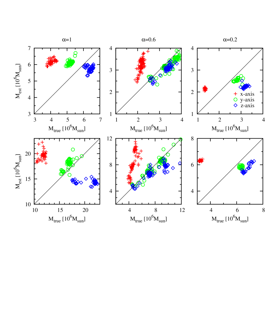
Figure 10: The same as Figure 4 but using data only for stars in Pop 1 (upper panel) and only in Pop 2 (lower panel).

To estimate the masses and slopes of the mass distribution (see the following section) we also need to measure the line-of-sight velocity dispersions of the stars belonging to each population within their respective half-light radii $R_{{\rm h},1}$ and $R_{{\rm h},2}$. These velocity dispersions are plotted as dotted and dashed lines in Figure 8 as a function of time. Interestingly, the velocity dispersions follow the hierarchy of half-light radii: the values of $\sigma_{\rm los}$ for the more concentrated Pop 1 are always smaller and for the more extended Pop 2 larger than the dispersion for all stars for all lines of sight and all $\alpha$. The only exception occurs for $\alpha=1$ and observation along the shortest $z$ axis of the stellar component, where the values of $\sigma_{\rm los}$ are very similar for all populations. This can be understood by referring to Figure 9 where we show examples of the line-of-sight velocity dispersion profiles for selected outputs, at times $t=9.7$, 8.95 and 4.9 Gyr, for $\alpha=1,0.6$ and 0.2, respectively (the same outputs were used in Figure 6) and different lines of sight.

For all cases the velocity dispersion profile decreases with the projected radius $R$ in the region of $R$ we probe, although more steeply for the less concentrated populations. In addition, the velocity dispersion profile for Pop 1 is always below the other two, as expected from the single-value measurements of $\sigma_{\rm los}$ shown in Figure 8 (an effect also noticed by McConnachie, Peñarrubia & Navarro 2007). Although the profiles show similar behaviour for all $\alpha$ and lines of sight, the single values used in the mass estimator and shown in Figure 8 depend also on the actual half-light radius within which they are measured. In Figure 9 we indicate the corresponding values of $R_{\rm h}$ by vertical lines of the same type as used to plot the dispersion profiles. The hierarchy of half-light radii is a little different for different $\alpha$ and lines of sight, for example for $\alpha=1$ the differences between the values of $R_{\rm h}$ for different populations grow systematically when going from observation along the $x$ to $z$ axis (see the vertical lines in the left-column plots of Figure 9), which results in values of averaged $\sigma_{\rm los}$ becoming similar for all populations. This behaviour is a little different for $\alpha=0.6$ and 0.2 because then the dwarfs are more prolate than triaxial (see also axis ratios in Figure 3).

In order to verify how working with sub-populations affects the mass estimates, we performed a similar comparison of estimated versus true masses as was done using all stars in the previous section. First, we calculated the masses from estimator (3) for each population separately, using the measured values of half-light radii $R_{{\rm h},1}$ and $R_{{\rm h},2}$ and the corresponding velocity dispersions. Then, we measured the actual masses of the simulated dwarfs within the half-light radius of a given population. The two measurements are compared in Figure 10 where the two rows show results for Pop 1 and Pop 2 respectively. The corresponding values of $M_{\rm est}/M_{\rm true}$ for the two populations (means and dispersions) are given in the second and third row for each $\alpha$ in Table 1. We see that, as in the case of using all stars, masses are always overestimated when the observation is along the $x$ axis of the stellar component and underestimated if the observation is along $z$. In particular, for observations along $x$, when using the data for Pop 2 (Pop 1) the mass is more (less) overestimated than for all stars. In addition, some bias also occurs for the line of sight along the intermediate axis $y$ for $\alpha=1$.

In Figures 11 and 12 we look again at the dependence of $M_{\rm est}/M_{\rm true}$ found for the two populations on the dwarf properties at a given stage, in terms of $V/\sigma$, $\beta$ and $c/a$. The trends with these parameters turn out to be similar as for the whole population of stars, namely $M_{\rm est}/M_{\rm true}$ obtained for different lines of sight converge as dwarfs become more spherical.

5 Estimating slopes

In this section we finally measure the slopes of the mass distribution of our simulated dwarfs using the estimator proposed by WP11

$$\Gamma_{\rm est}=\frac{\Delta\log M}{\Delta\log r}=1+\frac{\log(\sigma^{2}_{\rm los,1}/\sigma^{2}_{\rm los,2})}{\log(R_{\rm h,1}/R_{\rm h,2})}$$ (4)

where $\sigma_{{\rm los},i}$ is the line-of-sight velocity dispersion measured within $R_{{\rm h},i}$ for the $i$-th population. The estimated slopes calculated in this way were then compared to those measured directly from the simulation data. This true value $\Gamma_{\rm true}$ is obtained by taking in $\Delta\log M$ in equation (4) the true masses within $r_{\rm h,1}=fR_{\rm h,1}$ and $r_{\rm h,1}=fR_{\rm h,1}$. This turns out to be equivalent to a high accuracy to the direct fitting of the mass slope of the simulated dwarfs at a radius equally distant from $r_{\rm h,1}$ and $r_{\rm h,2}$ in log $r$, that is at $\log r=(\log r_{\rm h,1}+\log r_{\rm h,2})/2$.

The estimated and true values of $\Gamma$ are compared in Figure 13. Interestingly, in spite of the large scatter in mass estimates obtained from the kinematic data for the two populations, the estimated $\Gamma$ values for a given $\alpha$ and line of sight are confined to a very tight region. This demonstrates that the scatter in masses partially cancels out in the estimator (4) and thus speaks in favour of the method. However, $\Gamma_{\rm est}$ can be overestimated as well as underestimated depending on the line of sight and in particular it is always overestimated if the line of sight is along the longest axis of the stellar distribution. The exact values of the means and dispersions of $\Gamma_{\rm est}/\Gamma_{\rm true}$ are given in the fourth row for each $\alpha$ in Table 1.

Let us note that the agreement between $\Gamma_{\rm est}$ and $\Gamma_{\rm true}$ is best and almost perfect for the dwarfs observed along the intermediate $y$ axis of the stellar component, similarly as in the case of mass estimates. Interestingly, the behaviour of $\Gamma_{\rm est}/\Gamma_{\rm true}$ for observations along the $z$ axis is different for different $\alpha$. In particular, the ratio is below unity for $\alpha=1$, of the order of unity for $\alpha=0.6$ and above unity $\alpha=0.2$. This anomalous behaviour of the $\alpha=0.2$ case can be traced to a slightly bigger difference between $\sigma^{2}_{\rm los,1}$ and $\sigma^{2}_{\rm los,2}$ for observation along $z$ compared to $y$ axis (see Figure 8). While the differences between $R_{\rm h,1}$ and $R_{\rm h,2}$ are similar for the two lines of sight, and thus $\Gamma_{\rm true}$ values are similar, the difference in velocity dispersion of the two populations results in a larger $\Gamma_{\rm est}$ for the observation along $z$.

Before we conclude, let us again look at the dependence of the ratio $\Gamma_{\rm est}/\Gamma_{\rm true}$ on the properties of the dwarf: the amount of rotation, anisotropy and shape (Figure 14). The trends turn out to be similar as in the case of mass estimates for the whole population: $\Gamma_{\rm est}/\Gamma_{\rm true}$ tend to unity for more spherical stellar components.

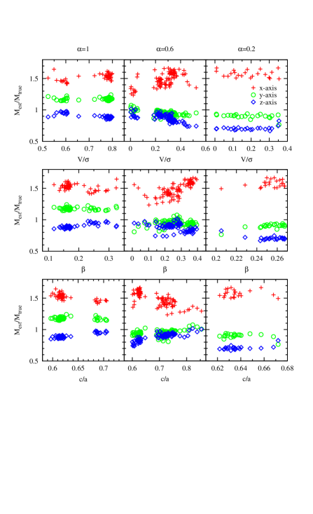
Figure 11: The same as Figure 5 but for the more concentrated stellar population Pop 1.

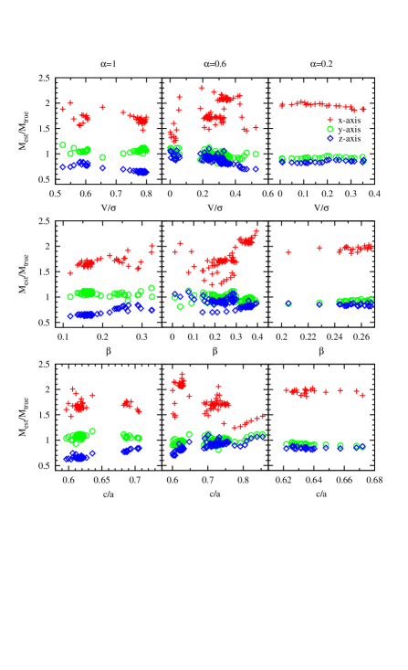
Figure 12: The same as Figure 5 but for the less concentrated stellar population Pop 2.

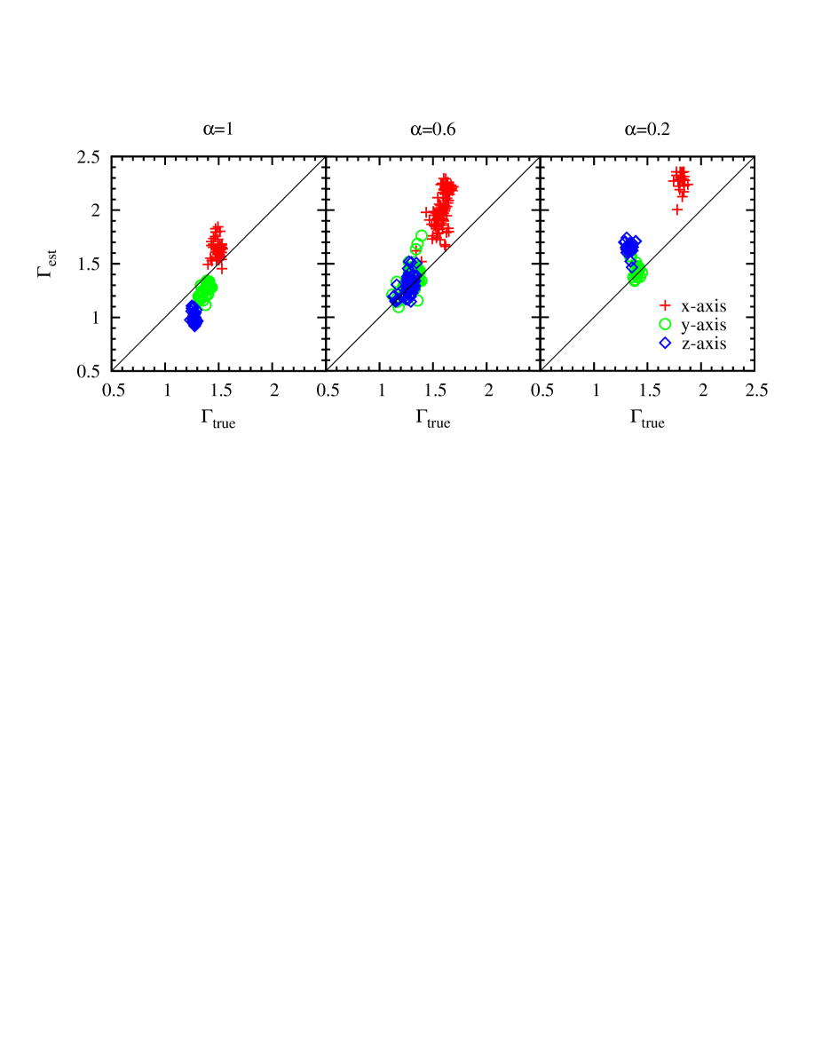
Figure 13: Comparison between the mass slopes $\Gamma$ obtained using estimator (4) and by direct measurement of masses at the two half-light radii in the simulation. The three panels from the left to the right show results for $\alpha=1,0.6$ and 0.2, respectively, and the diagonal line in each panel corresponds to the equality of the $\Gamma$ values. Symbols of different shape and colour indicate measurements derived from observations performed along different lines of sight: $x$ (longest axis of the stellar component), $y$ (intermediate axis) and $z$ (shortest axis).

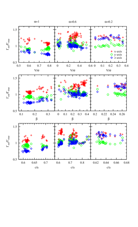
Figure 14: The ratio of the estimated to true slope $\Gamma$ as a function of the amount of rotation $V/\sigma$ (upper row), the anisotropy parameter $\beta$ (middle row) and shape in terms of the ratio of the shortest to longest axis of the stellar component $c/a$ (lower row). The columns from the left to the right show results for $\alpha=1,0.6$ and 0.2, respectively. Symbols of different shape and colour indicate observations performed along different lines of sight: $x$ (longest axis of the stellar component), $y$ (intermediate axis) and $z$ (shortest axis).

6 Discussion

Using collisionless $N$-body simulations of dwarf galaxies orbiting the Milky Way we created numerical models of dwarfs with non-spherical stellar components and measured their properties as is usually done in observations of real dSph galaxies in the Local Group. The use of high-resolution simulations allowed us to construct kinematic samples almost free of the usual statistical errors associated with observational uncertainties. The stars in the simulated dwarfs have positions and velocities known to arbitrary accuracy and the membership of the stars in a given population is known by definition. The statistical errors on the inferred values of the half-light radii and velocity dispersions, such as sampling errors, are very small due to a large number of stars available. These facts allowed us to study the systematic errors involved in the determination of the masses and density slopes of the dwarfs.

We have demonstrated that the inferred values of the mass contained within a radius of the order of a half-light radius of the stars can be over- or underestimated depending on the line of sight along which the observation is performed. In particular, the masses are always larger than the real ones by up to a factor of two if the dwarfs are observed along the longest axis of the stellar component. When observed along the shortest axis, the masses are underestimated by at most 30 percent. The bias is weakest for the observation along the intermediate axis and in this case the masses are recovered with a very good accuracy.

The most important conclusion of this work is related to the inferences concerning the slope of mass distribution in dSph galaxies, an issue which has attracted a lot of attention among the modellers in recent years. Using the same mock data samples as were used to study the accuracy of mass estimates we studied the reliability of the method recently proposed by WP11 to infer the slope of mass distribution $\Gamma$. Our main result is summarized in Figure 13. We demonstrated that the slope of mass distribution estimated using this method can be under- and overestimated depending on the line of sight along which the observation is performed. This has immediate consequences for the inferences concerning the slope of the density profile in dSph galaxies.

Let us define the limiting inner slope of the density profile as $\gamma(r\rightarrow 0)=\gamma_{0}$. The analogous value of the mass slope will be $\Gamma(r\rightarrow 0)=\Gamma_{0}$. As discussed by WP11, in the limit of small radii

$$\gamma_{0}=3-\Gamma_{0}<3-\Gamma$$ (5)

because for any radius $r>0$ we have $\Gamma_{0}>\Gamma(r)$. For example, taking $\Gamma_{\rm est}=2.3$ found for $\alpha=0.6$ and observation along the $x$ axis (see the middle panel Figure 13) leads to the constraint $\gamma_{0}<0.7$ while taking the corresponding true value $\Gamma_{\rm true}=1.6$ gives $\gamma_{0}<1.4$, thus a result entirely consistent with the presence of an inner cusp. Therefore using an overestimated value of $\Gamma_{\rm est}$ in equation (5) may lead us to infer a presence of a core-like profile when no such profile is really there.

We further illustrate this conclusion by showing in the two lower panels of Figure 2 and in Figure 15 the actual slopes of the total (dark matter and stars) density and mass profiles, respectively. The slopes are shown as a function of time for radii bracketing our range of half-light radii (0.2 and 0.5 kpc) for $\alpha=0.2$, 0.6 and 1. As we can see from Figure 2, at $r=0.2$ even for $\alpha=0.2$ the total density slope $-\gamma<-1$ at most times until the third pericentre and thus indeed no core is present at this scale. Note that $r=0.2$ is of the order of 3-4 softening scales for dark matter particles in our simulations and thus is the smallest scale where we can reliably determine the total density profile. The method of WP11 obviously is supposed to give the slope of the total mass profile and the inferences concerning the most interesting question of the slope of the dark matter distribution can only be made under the assumption that dark matter dominates strongly over stars everywhere in the dwarf galaxy. This may not always be the case, especially in the central part of dwarfs. For our simulated dwarfs the slopes do differ as confirmed by comparison between the first and third row panels of Figure 2.

Figure 15 can also be viewed as a consistency check for the $\Gamma_{\rm true}$ values shown in Figure 13. The values of $\Gamma_{\rm true}$ should fall between the values shown in the two panels of Figure 15 since $\Gamma_{\rm true}$ are measured at radii from the range bracketed by half-light radii of the two stellar populations and these are typically between 0.2 and 0.5 kpc (see Figure 7). Indeed, for the selected outputs we used the values of $\Gamma_{\rm true}$ from Figure 13 are in the range $1.2-1.5$, $1.1-1.7$ and $1.3-1.8$ respectively for $\alpha=1$, 0.6 and 0.2, in agreement with values plotted in Figure 15.

WP11 applied their method to the data for the Fornax and Sculptor dSph galaxies obtaining $\Gamma$ values of 2.61 and 2.95 with a rather small error of the order of 0.4. Thus, according to equation (5), they inferred the presence of cores in these galaxies: $\gamma_{0}<0.39$ and $\gamma_{0}<0.05$. Given our results, these inferences can be systematically biased towards the presence of the core if the dwarfs are observed along the major axis of the stellar component. Our results thus weaken the tension between the findings of WP11 and recent results of simulations (Governato et al. 2012) where such extended cores tend to form only in significantly more massive galaxies.

Figure 15: The evolution of the slope of the total (dark matter + stars) mass profile in time measured at the radius $r=0.2$ (upper panel) and $r=0.5$ kpc (lower panel) from the centre of the dwarf. The solid, dashed and dotted lines show slopes measured for dwarfs with haloes of different initial inner slope $\alpha=1,0.6$ and 0.2, respectively. Thin vertical lines indicate pericentre passages.

Table 1: Estimated masses and slopes versus true values.

Quantity	along $x$	along $y$	along $z$
		$\alpha=1$
$M_{\rm est}/M_{\rm true}(fR_{\rm h})$	$1.61\pm 0.08$	$1.05\pm 0.03$	$0.72\pm 0.06$
$M_{\rm est}/M_{\rm true}(fR_{\rm h,1})$	$1.52\pm 0.05$	$1.18\pm 0.02$	$0.90\pm 0.03$
$M_{\rm est}/M_{\rm true}(fR_{\rm h,2})$	$1.68\pm 0.09$	$1.07\pm 0.04$	$0.69\pm 0.07$
$\Gamma_{\rm est}/\Gamma_{\rm true}(fR_{\rm h,i})$	$1.10\pm 0.06$	$0.92\pm 0.03$	$0.77\pm 0.04$
		$\alpha=0.6$
$M_{\rm est}/M_{\rm true}(fR_{\rm h})$	$1.72\pm 0.22$	$0.96\pm 0.05$	$0.87\pm 0.07$
$M_{\rm est}/M_{\rm true}(fR_{\rm h,1})$	$1.48\pm 0.11$	$0.95\pm 0.04$	$0.88\pm 0.06$
$M_{\rm est}/M_{\rm true}(fR_{\rm h,2})$	$1.81\pm 0.25$	$0.98\pm 0.06$	$0.88\pm 0.08$
$\Gamma_{\rm est}/\Gamma_{\rm true}(fR_{\rm h,i})$	$1.25\pm 0.11$	$1.05\pm 0.06$	$1.01\pm 0.05$
		$\alpha=0.2$
$M_{\rm est}/M_{\rm true}(fR_{\rm h})$	$1.86\pm 0.04$	$0.91\pm 0.02$	$0.81\pm 0.02$
$M_{\rm est}/M_{\rm true}(fR_{\rm h,1})$	$1.57\pm 0.06$	$0.90\pm 0.04$	$0.71\pm 0.03$
$M_{\rm est}/M_{\rm true}(fR_{\rm h,2})$	$1.95\pm 0.04$	$0.92\pm 0.02$	$0.85\pm 0.02$
$\Gamma_{\rm est}/\Gamma_{\rm true}(fR_{\rm h,i})$	$1.25\pm 0.05$	$1.03\pm 0.05$	$1.24\pm 0.06$

Our results suggest that the method could be more reliable and the systematics of the uncertainties could be more under control if we knew the orientation of the studied object with respect to our line of sight. Although most of dSph galaxies are known to be non-spherical from their surface density maps, their orientation remains unknown. If most of the dSphs indeed formed via tidal stirring, they should remain non-spherical until the present except for those that evolved on tight enough orbits for a long enough time (Kazantzidis et al. 2011). The orientation of the major axis of the stellar component should then be random, as the dwarfs are supposed to tumble with a period much shorter than the orbital period of their motion around the Milky Way (see figure 4 in Łokas et al. 2011).

An interesting exception where the orientation of the dwarf could be determined is the case of the Sagittarius dwarf. According to the model proposed by Łokas et al. (2010b) the dwarf is now close to the second pericentre of its orbit around the Milky Way and forms a bar oriented perpendicular to our line of sight. The Sagittarius dwarf could thus become a promising target for the unbiased application of the method but the case requires further studies to confirm its orientation and identify multiple stellar populations among its stars.

Despite the biases inherent in this method when applied to a single dSph, which is necessarily observed along one line of sight, it can still be useful when applied to a larger sample of nearby dSph galaxies which should be oriented randomly with respect to our position in the Galaxy. The biases are then expected to diminish and a mean result can be closer to the truth than for a single object. This averaging may work if the dwarfs were all formed in a similar fashion and possess similar properties, in particular in terms of the dark matter distribution. Given their different masses, luminosities and star formation histories this may not however be the case.

References

- [Breddels et al.(2012)] Breddels M. A., Helmi A., van den Bosch R. C. E., van de Ven G., Battaglia G., 2012, submitted to MNRAS, arXiv:1205.4712
- [Bruzual & Charlot(2003)] Bruzual G., Charlot S., 2003, MNRAS, 344, 1000
- [Chaname et al.(2008)] Chanamé J., Kleyna J., van der Marel R., 2008, ApJ, 682, 841
- [Cole et al.(2012)] Cole D. R., Dehnen W., Read J. I., Wilkinson M. I., 2012, MNRAS, 426, 601
- [de Blok et al.(2001)] de Blok W. J. G., McGaugh S. S., Rubin V. C., 2001, AJ, 122, 2396
- [Diemand et al.(2007)] Diemand J., Kuhlen M., Madau P., 2007, ApJ, 667, 859
- [Goerdt et al.(2006)] Goerdt T., Moore B., Read J. I., Stadel J., Zemp M., 2006, MNRAS, 368, 1073
- [Governato et al.(2010)] Governato F. et al., 2010, Nature, 463, 203
- [Governato et al.(2012)] Governato F. et al., 2012, MNRAS, 422, 1231
- [Jardel & Gebhardt(2012)] Jardel J. R., Gebhardt K., 2012, ApJ, 746, 89
- [Kazantzidis et al.(2004)] Kazantzidis S., Mayer L., Mastropietro C., Diemand J., Stadel J., Moore B., 2004, ApJ, 608, 663
- [Kazantzidis et al.(2011)] Kazantzidis S., Łokas E. L., Callegari S., Mayer L., Moustakas L. A., 2011, ApJ, 726, 98
- [Kazantzidis et al.(2013)] Kazantzidis S., Łokas E. L., Mayer L., 2013, ApJ, 764, L29
- [Klimentowski et al.(2007)] Klimentowski J., Łokas E. L., Kazantzidis S., Prada F., Mayer L., Mamon G. A., 2007, MNRAS, 378, 353
- [Klimentowski et al.(2009a)] Klimentowski J., Łokas E. L., Kazantzidis S., Mayer L., Mamon G. A., 2009a, MNRAS, 397, 2015
- [Klimentowski et al.(2009b)] Klimentowski J., Łokas E. L., Kazantzidis S., Mayer L., Mamon G. A., Prada F., 2009b, MNRAS, 400, 2162
- [Klimentowski et al.(2010)] Klimentowski J., Łokas E. L., Knebe A., Gottlöber S., Martinez-Vaquero L. A., Yepes G., Hoffman Y., 2010, MNRAS, 402, 1899
- [Lokas(2002)] Łokas E. L., 2002, MNRAS, 333, 697
- [Lokas & Mamon(2003)] Łokas E. L., Mamon G. A., 2003, MNRAS, 343, 401
- [Lokas et al.(2005)] Łokas E. L., Mamon G. A., Prada F., 2005, MNRAS, 363, 918
- [Lokas et al.(2010a)] Łokas, E. L., Kazantzidis, S., Klimentowski, J., Mayer, L., & Callegari, S. 2010a, ApJ, 708, 1032
- [Lokas et al.(2010b)] Łokas, E. L., Kazantzidis, S., Majewski, S. R., Law, D. R., Mayer, L., & Frinchaboy, P. M. 2010b, ApJ, 725, 1516
- [Lokas et al.(2011)] Łokas E. L., Kazantzidis S., Mayer L., 2011, ApJ, 739, 46
- [Lokas et al.(2012a)] Łokas E. L., Majewski S. R., Kazantzidis S., Mayer L., Carlin J. L., Nidever D. L., Moustakas L. A., 2012a, ApJ, 751, 61
- [Lokas et al.(2012b)] Łokas E. L., Kazantzidis S., Mayer L., 2012b, ApJ, 751, L15
- [Lokas et al.(2012c)] Łokas E. L., Kowalczyk K., Kazantzidis S., 2012c, in Bono G., de Grijs R., Omizzolo A., eds, Proc. EWASS 2012 Symp. 6, Stellar Populations 55 years after the Vatican Conference. Memorie della Societa Astronomica Italiana, in press, arXiv:1212.0682
- [Mateo(1998)] Mateo M. L., 1998, ARA&A, 36, 435
- [McConnachie et al.(2007)] McConnachie A. W., Peñarrubia J., Navarro J. F., 2007, MNRAS, 380, L75
- [Mayer et al.(2001)] Mayer L., Governato F., Colpi M., Moore B., Quinn T., Wadsley J., Stadel J., Lake G., 2001, ApJ, 559, 754
- [Mayer et al.(2007)] Mayer L., Kazantzidis S., Mastropietro C., Wadsley J., 2007, Nature, 445, 738
- [Mo et al.(1998)] Mo H. J., Mao S., White S. D. M., 1998, MNRAS, 295, 319
- [Navarro et al.(1997)] Navarro J. F., Frenk C. S., White S. D. M., 1997, ApJ, 490, 493 (NFW)
- [Oh et al.(2011)] Oh S.-H. et al., 2011, AJ, 142, 24
- [Sanchez-Conde et al.(2007)] Sánchez-Conde M. A., Prada F., Łokas E. L., Gómez M. E., Wojtak R., Moles M., 2007, Phys. Rev. D, 76, id. 123509
- [Spergel & Steinhardt(2000)] Spergel D. N., Steinhardt P. J., 2000, Phys. Rev. Letters, 84, 3760
- [Stadel(2001)] Stadel J. G., 2001, PhD thesis, Univ. of Washington
- [Vogelsberger et al.(2012)] Vogelsberger M., Zavala J., Loeb A., 2012, MNRAS, 423, 3740
- [Walker & Penarrubia(2011)] Walker M. G., Peñarrubia J., 2011, ApJ, 742, 20
- [Widrow & Dubinski(2005)] Widrow L. M., Dubinski J., 2005, ApJ, 631, 838
- [Wolf et al.(2010)] Wolf J., Martinez G. D., Bullock J. S., Kaplinghat M., Geha M., Muñoz R. R., Simon J. D., Avedo F. F., 2010, MNRAS, 406, 1220