Self-Stabilizing Balancing Algorithm
for Containment-Based Trees

Abstract

Containment-based trees encompass various handy structures such as B+-trees, R-trees and M-trees. They are widely used to build data indexes, range-queryable overlays, publish/subscribe systems both in centralized and distributed contexts. In addition to their versatility, their balanced shape ensures an overall satisfactory performance. Recently, it has been shown that their distributed implementations can be fault-resilient. However, this robustness is achieved at the cost of unbalancing the structure. While the structure remains correct in terms of searchability, its performance can be significantly decreased. In this paper, we propose a distributed self-stabilizing algorithm to balance containment-based trees.

I Introduction

Several tree families are based on a containment relation. Examples include B+-trees [1], R-trees [2], and M-trees [3]. They are respectively designed to handle intervals, rectangles, and balls. Their logarithmic height ensures good performance for basic insertion/deletion/search primitives. Basically they rely on a partial order on node labels. They can be specified as follows:

1. Tree nature. The graph is acyclic and connected.

2. Containment relation. Every non-root node $n$ satisfies $label(n)\sqsubseteq label(father(n))$.

3. Bounded degrees. The root has between 2 and $M$ children, each internal node has between $m$ and $M$ children ($M\geq 2m$).

4. Balanced shape. All leaves are at the same level.

In a distributed context, no node has a global knowledge of the system as each node has only access to its local information. As a consequence, the aforementioned invariants should be expressed as “local” constraints; at the level of a node. Operations preserving or restoring those invariants should also be “as local as possible”.

Preserving the tree nature has been addressed in previous work [4, 5, 6]. It is tightly related to the distribution model of the structure, the centralized case being far less stressing. The containment relation is easy to preserve as node labels can be “enlarged” or “shrunk”. The bounded node degrees are ensured with $split$ or $collapse$ primitives when a node has too many or too few children, respectively. The balanced shape of the tree is especially important in terms of performance; in conjunction with node degree bounds, it ensures that the tree has logarithmic height. A number of approaches have been proposed in the literature in order to balance tree overlays. However, these solutions have many limitations in particular when applied to containment-based tree overlays.

The works in [4, 6] have the extra property of being self-stabilizing. A self-stabilizing system, as introduced in [7], is guaranteed to converge to the intended behavior in finite time, regardless of the initial states of nodes. Self-stabilization [7] is a general technique to design distributed systems that can handle arbitrary transient faults.

Figure 1 shows the overlay lifecycle borrowed from [6]. Rectangles refer to states of the distributed tree. Transitions are labelled with events (join and faults) or algorithms (repair and balance) triggering them . Initially the tree is empty, then some peers join the overlay building a searchable tree. The balancing algorithm eventually balances the tree. In case of joins the tree may become unbalanced. In case of faults the tree may become disconnected. The repair algorithm eventually reconnects the tree and fixes containment relation. The distinction between searchable and balanced states emphasizes a separation of concerns between correction and performance. Basically repair is about correction, while balance is about performance. It is also interesting to point out that if the balance algorithm is self-stabilizing, then the join algorithm does not have to deal with performance. Moreover, if the repair algorithm is self-stabilizing, a peer quitting the overlay does not have to communicate with any other peer; departures can be handled as faults.

Figure 1: Containment-based tree overlay lifecycle. The overlay is balanced when all invariants are ensured, searchable when all but the fourth invariant are ensured, and disconnected when at least the tree nature invariant is violated.

I-A Related Work

DR-tree [4] is a distributed version of R-trees [2] developed to build a brokerless peer to peer publish/subscribe system. Each computer stores a leaf and some of its consecutive ancestors. The closer node to the root stored by a computer is called its “first node”. Each computer knows some ancestors of its first node; from its grand father to the root. The tree may become unbalanced in case of faults. When a computer detects that the computer storing the father of its first node is crashed, it broadcasts a message in the subtree starting from its first node. All leaves belonging to that subtree will be reinserted elsewhere starting from an ancestor of the crashed peer’s first node. As a consequence, no balancing primitive is used. However, up to half of the nodes of the tree may have to be reinserted (if faults occur near the root).

SDR-tree [8] is an indexing structure distributed amongst a cluster of servers. Its main aim is to provide efficient and scalable range queries. It builds balanced full binary trees satisfying containment relation. Each computer stores exactly one leaf and one internal node. Instead of classic $split$ and $collapse$ operations, this paper extensively uses subtree heights to guarantee the balanced shape of the structure. They adapt the concept of rotation [9] to multidimensional data. However they don’t mention how to repair the structure in case of crashes.

VBI [5], a sequel of BATON [10], is a framework to build distributed spatial indexes on top of binary trees. It provides default implementations for all purely structural concerns of binary trees: maintaining father and children links, rotations, etc. Developers only have to focus on several operations, mostly related to node labeling (such as $split$ and $collapse$). However, despite their interesting approach of mapping any tree on a binary one, they do not provide a handy way to parameterize the system. While modifying node degree bounds should be a simple way to tune system performances, the fixed degree of the core structure (a tradeoff between reusability and performance) cannot be bypassed.

The solution proposed in [6] also deals with full binary trees satisfying containment relation. The distribution is the same as in the SDR-tree; each computer stores exactly one leaf and one internal node. The core contribution of this paper is to prove that if the leaf and the internal node held by each machine are randomly chosen, then the graph between computers (namely, the communication graph) is very unlikely to be disconnected in case of faults. More precisely, faults disconnect the logical structure, but not the communication graph. This paper proposes an algorithm exploiting the connectivity of the communication graph to repair the logical structure restoring the tree nature, containment relation and bounded node degrees. This approach is shown as much cheaper than [4], both in terms of recovery time and cost in messages. However the restored tree can be slightly unbalanced and the restoration of its shape is not addressed in the paper.

The algorithm proposed in [6] has the desirable property of being self-stabilizing. There exist several distributed, self-stabilizing algorithms in the literature that maintain a global property based on node labels, e.g., [11, 12, 13]. The solutions in [11, 12] achieve the required property (resp. Heap and BST) by reorganizing the key in the tree. They have no impact on the tree topology. The solution in [13] arranges both node labels (or, keys) and the tree topology. None of the above self-stabilizing solutions deal with the balanced property.

I-B Contribution

In this paper, we first show that edge swapping can be used as a balancing primitive. Then we propose a distributed self-stabilizing algorithm balancing any containment-based tree, such as B+-trees [1], R-trees [2] and M-trees [3]. Our algorithm can be used in [8, 6] to enhance the performance of repaired trees, or in [5, 10] as a “core” balancing mechanism. We further prove the correctness of the algorithm and investigate its practical convergence speed via simulations.

I-C Roadmap

In Section II, we argue that edge swapping is practically better suited than rotations to balance containment-based trees. In Section III, we present the model we use to describe our algorithm. In Section IV, we propose a distributed self-stabilizing algorithm that relies on edge swapping to balance any containment-based tree. In the same section, we prove the termination and correctness of the algorithm. In Section V, we investigate the practical termination time of our algorithm via simulations. Section VI contains some concluding remarks and possible directions for future work.

II Balancing Primitive

Let $\alpha\in\mathbb{N}$. A tree is balanced iff all its nodes are balanced. A node is balanced iff the heights of any pair of its children differ at most by $\alpha$. In the remainder of this paper, we make two assumptions:

• $\alpha\geq 1$.

• each non-leaf node has at least two children.

The assumption on $\alpha$ is weaker than those of [8, 6, 5] and still ensures logarithmic height of the tree [14]. The degree assumption is also weaker than those of [8, 6, 5] and allows more practical tree configurations.

Basically, a balancing primitive is an operation that eventually reduces the difference between the heights of some subtrees by modifying several links of the tree. Those link modifications may have some semantic impact if they break node labeling invariants.

II-A Rotation

In BST [15] and AVL [9], the well known rotation primitive is used to ensure the balanced shape of the tree. However, when dealing with structures relying on partially ordered data, rotations do have a semantic impact. Moreover, in a distributed context, if a node $n$ and its father or grandfather concurrently execute rotations, they may both “write” $father(n)$. It follows that the use of distributed rotations requires synchronization to preserve tree structure.

II-B Edge swapping

(a) Swapping $(a,c)$ and $(b,e)$…

(b) …to $(a,e)$ and $(b,c)$

Figure 2: An example of edge swapping. The fathers of $c$ and $e$ are modified. The label of $b$ needs to be updated.

Given two edges $(a,b)$ and $(c,d)$, swapping them consists in exchanging their tails (resp. heads). Formally, $swap((a,b),(c,d))$ modifies the edges of the graph as follows: $E(G)\coloneqq E(G)-\{(a,b),(c,d)\}+\{(a,d),(c,b)\}$. Figure 2 contains an illustration. With the algorithm that we present in Section IV, concurrent swaps cannot conflict. The use of this balancing primitive is thus more suitable in a distributed context.

III Model

In this paper, we consider the classical local shared memory model, known as the state model, that was introduced by Dijkstra [7]. In this model, communications between neighbours are modeled by direct reading of variables instead of exchange of messages. The program of every node consists in a set of shared variables (henceforth referred to as variable) and a finite number of actions. Each node can write in its own variables and read its own variables and those of its neighbors. Each action is constituted as follows:

$<Label>::<Guard>$ $<Statement>$

The guard of an action is a boolean expression involving the variables of a node $u$ and its neighbours. The statement is an action which updates one or more variables of $u$. Note that an action can be executed only if its guard is true. Each execution is decomposed into steps.

The state of a node $u$ is defined by the value of its variables. It consists of the following pieces of information:

• An integer value which we call the height value or height information of node $u$.

• Two arrays that contain the IDs of the children of $u$ and their height values.

For the sake of generality, we do not make any assumptions about the number of bits available for storing height information, thus the height value of a node can be an arbitrarily large (positive or negative) integer.

The configuration of the system at any given time $t$ is the aggregate of the states of the individual nodes. We will sometimes use the term “configuration” to refer to the rooted tree formed by the nodes.

Definition 1

We denote by $\mathcal{C}(t)$ the configuration of the system at time $t\geq 0$. For a node $u$, we denote by $h_{u}(t)$ the value of its height variable in $\mathcal{C}(t)$, by $h^{\star}_{u}(t)$ its actual height in the tree in $\mathcal{C}(t)$, by $\mathcal{S}_{u}(t)$ the set of children of $u$ in $\mathcal{C}(t)$, and by $\mathcal{S}^{\star}_{u}(t)$ the set of nodes in the subtree rooted at $u$ in $\mathcal{C}(t)$.

Let $\mathcal{C}(t)$ be a configuration at instant $t$ and let $I$ be an action of a node $u$. $I$ is enabled for $u$ in $\mathcal{C}(t)$ if and only if the guard of $I$ is satisfied by $u$ in $\mathcal{C}(t)$. Node $u$ is enabled in $\mathcal{C}(t)$ if and only if at least one action is enabled for $u$ in $\mathcal{C}(t)$. Each step consists of two sequential phases executed atomically: ($i$) Every node evaluates its guard; ($ii$) One or more enabled nodes execute their enabled actions. When the two phases are done, the next step begins. This execution model is known as the distributed daemon [16]. To capture asynchrony, we assume a semi-synchronous scheduler which picks any non-empty subset of the enabled nodes in the current configuration and executes their actions simultaneously. We do not make any fairness assumptions, thus the scheduler is free to effectively ignore any particular node or set of nodes as long as there exists at least one other node that can be activated.

Definition 2

We refer to the activation of a non-empty subset $A$ of the enabled nodes in a given configuration as an execution step. If $\mathcal{C}$ is the configuration of the system before the activation of $A$ and $\mathcal{C}^{\prime}$ is the resulting configuration, we denote this particular step by $\mathcal{C}\longrightarrow_{A}\mathcal{C}^{\prime}$. An execution starting from an initial configuration $\mathcal{C}_{0}$ is a sequence $\mathcal{C}_{0}\longrightarrow_{A_{1}}\mathcal{C}_{1}\longrightarrow_{A_{2}}\mathcal{C}_{2}\longrightarrow\dots$ of execution steps. Time is measured by the number of steps that have been executed. An execution is completed when it reaches a configuration in which no node is enabled. After that point, no node is ever activated.

If a node was enabled before a particular execution step, was not activated in that step, and is not enabled after that step, then we say that it was neutralized after that step.

Definition 3

Given a particular execution, an execution round (or simply round) starting from a configuration $\mathcal{C}$ consists of the minimum-length sequence of steps in which every enabled node in $\mathcal{C}$ is activated or neutralized at least once.

Remark 1

To simplify the presentation, we will assume throughout the rest of the paper that the arrays containing the IDs of the children of each node and copies of their height values are consistent with the height values stored by the children themselves in the current configuration of the system. It should be clear that maintaining these copies up to date can be achieved with a constant overhead per execution step.

IV Self-Stabilizing Balancing Solution

In this section, we present our self-stabilizing algorithm for balancing containment-based trees, we provide some termination properties, and we prove that any execution converges to a balanced tree.

Assuming that each node knows the correct heights of its subtrees, a very simple distributed self-stabilizing algorithm balances the tree: each node uses the swap operation whenever two of its children heights are “too different”. However, in a distributed context, height information may be inaccurate. This inaccuracy could lead the aforementioned naive balancing algorithm to make some “wrong moves.” For example, in Figure 2, assume that $c$ “thinks” that its own height is $4$ and $e$ “thinks” that its own height is $9$ while their actual heights are respectively $10$ and $8$; the illustrated swap would actually unbalance the tree. On one hand, maintaining heights in a self-stabilizing fashion is easy and ensures that height information will eventually be correct. On the other hand, no node can know when height information is correct; as a consequence, height maintenance and balancing have to run concurrently. But their concurrent execution raises an obvious risk: the swap operation modifies the tree structure and could thus compromise the convergence of the height maintenance subprotocol.

Basically, the algorithm that we propose in this section consists of two concurrent actions: one maintaining heights, the other one balancing the tree. We formalize both actions and prove that their concurrent execution converges to a balanced tree.

IV-A Algorithm

At any time $t$, each node $u$ is able to evaluate the following functions and predicates for itself and its children:

• $\mathrm{max}(x)$: returns any $v\in\mathcal{S}_{x}(t)$ such that $h_{v}(t)=\max_{w\in\mathcal{S}_{x}(t)}h_{w}(t)$. If $x$ is a leaf, returns $\bot$ (undefined).

• $\mathrm{min}(x)$: returns any $v\in\mathcal{S}_{x}(t)$ such that $h_{v}(t)=\min_{w\in\mathcal{S}_{x}(t)}h_{w}(t)$. If $x$ is a leaf, returns $\bot$.

• $\mathrm{stable}(x)$: returns true if and only if $h_{x}(t)=1+\max_{w\in\mathcal{S}_{x}(t)}h_{w}(t)$. If $x$ is a leaf, returns true if and only if $h_{x}(t)=0$.

• $\mathrm{balanced}(x)$: returns true if and only if for all $z,z^{\prime}\in\mathcal{S}_{x}(t)$, $|h_{z}(t)-h_{z^{\prime}}(t)|\leq\alpha$.

When there are more than one possible return values for $\mathrm{max}(x)$ and $\mathrm{min}(x)$, an arbitrary choice is made. For simplicity, we can consider that the candidate node with the smallest ID is returned, although this will not be crucial for our results.

Each node $u$ executes the algorithm in Figure 3 (the value of $\mathrm{stable}(\bot)$ is assumed to be false).

Guard	Statement
G1 $\neg\mathrm{stable}(u)$	S1 $h_{u}\coloneqq 1+\max_{w\in\mathcal{S}_{u}}h_{w}$ (or $h_{u}\coloneqq 0$ if $u$ is a leaf)
G2 $\mathrm{stable}(u)\wedge\mathrm{stable}(\mathrm{max}(u))\wedge$ $\neg\mathrm{balanced}(u)$	S2 swap edges $(u,\mathrm{min}(u))$ and $(\mathrm{max}(u),\mathrm{max}(\mathrm{max}(u))$

Figure 3: Distributed self-stabilizing balancing algorithm

Note that the guards G1 and G2 are mutually exclusive and, by definition, the height update action effectively has priority over the edge swapping action. We say that a node is enabled for a height update if G1 is true, or enabled for a swap if G2 is true.

When a node $u$ performs a swap, four nodes are involved: $u$ itself, $\mathrm{max}(u)$, $\mathrm{min}(u)$, and $\mathrm{max}(\mathrm{max}(u))$. We refer to these nodes as the source, the target, the swap-out, and the swap-in nodes of the swap, respectively.

The following proposition can be proved directly from the definitions. We state it without proof.

Proposition 1

If $\mathcal{C}$ is a rooted tree with root $r$, then after any execution step $\mathcal{C}\longrightarrow_{A}\mathcal{C}^{\prime}$, $\mathcal{C}^{\prime}$ is still a directed tree with root $r$.

IV-B Termination Properties

In the following section, we will prove that for any initial configuration, every possible execution is completed in a finite number of steps. For the moment, we give two properties of the resulting tree, assuming of course that the execution consists of a finite number of steps.

The proof of the following proposition can be found in Appendix -A.

Proposition 2

If the execution is completed, then in the final configuration $\mathcal{C}(t^{\star})$ all nodes are balanced and have correct height information.

The next proposition, regarding the height of the resulting tree, follows directly from the analysis in [14, Sections II and III]. In our case, the initial conditions of the recurrence studied in [14] are slightly different, but this does not affect the asymptotic behavior of the height.

Proposition 3

If the execution is completed in time $t^{\star}$, then in the final configuration $h^{\star}_{r}(t^{\star})=\mathcal{}(\log n)$, where $r$ is the root and $n$ is the number of nodes in the system.

IV-C Proof of Convergence

We give an overview of the proof with references to the appropriate appendices for the technical parts.

The concept of a “bad node” will be useful in the analysis of the algorithm.

Definition 4 (Bad nodes)

In a given configuration $\mathcal{C}(t)$, an internal node $u$ is a bad node if $h_{u}(t)\leq\max_{v\in\mathcal{S}_{u}(t)}h_{v}(t)$. A leaf is a bad node if $h_{u}(t)<0$.

Intuitively, a bad node is a node that “wants” to increase its height value. The proof of the following key lemma can be found in Appendix -B.

Lemma 4

If $\mathcal{C}(t)$ contains no bad nodes, then for all $t^{\prime}\geq t$, $\mathcal{C}(t^{\prime})$ contains no bad nodes.

It will be convenient to view any execution of the algorithm as consisting of two phases: The first phase starts from the initial configuration and ends at the first configuration in which the system is free of bad nodes. The second phase starts at the end of the first phase and ends at the first configuration in which no node is enabled, i.e., at the end of the execution. In view of Lemma 4, the system does not contain any bad nodes during the second phase. We will prove that each phase is concluded in a finite number of steps, starting from the second phase.

IV-C1 Second Phase

We prove convergence for the second phase by bounding directly the number of height updates and the number of swaps that may occur during that phase. The fact that there are no bad nodes in the second phase is crucial for bounding the number of height updates. It follows that the number of swaps also has to be bounded, since a long enough sequence of steps in which only swaps are performed incurs more height updates. The detailed proofs of these claims can be found in Appendix -C.

Lemma 5

Starting from a configuration with no bad nodes, no execution can perform an infinite number of height updates.

Lemma 6

Starting from a configuration with no bad nodes, no execution can perform an infinite number of swaps.

Lemmas 5 and 6 directly imply the following:

Theorem 7

In any execution, the second phase is completed in a finite number of steps.

IV-C2 First Phase

For the sake of presentation, it will be helpful to sometimes consider that the root of the tree has an imaginary father $\mathfrak{r}$, which is never enabled and always a bad node.

Definition 5 (Extended configuration)

We denote by $\tilde{\mathcal{C}}(t)$ an auxiliary extended configuration at time $t$, which is identical to $\mathcal{C}(t)$ except that the root node in $\mathcal{C}(t)$ has a new father node $\mathfrak{r}$ with $h_{\mathfrak{r}}(t)=-\infty$, for all $t\geq 0$.

The bad nodes induce a partition of the nodes of the extended configuration into components: each bad node belongs to a different component, and each non-bad node belongs to the component that contains its nearest bad ancestor.

Definition 6 (Partition into components)

For each bad node $b$ in $\tilde{\mathcal{C}}(t)$, the component $\mathcal{T}_{b}(t)$ is the maximal weakly connected directed subgraph of $\tilde{\mathcal{C}}(t)$ that has $b$ at its root and contains no other bad nodes.

A useful property of this partition is that it remains unchanged as long as the set of bad nodes remains the same. Therefore, in any sequence of steps in which the set of bad nodes remains the same, each component behaves similarly to a system that does not contain bad nodes. In particular, Lemmas 5 and 6 imply that each component is stabilized in finite time, and thus this sequence of steps cannot be infinite. For a complete substantiation of these claims, please refer to the proof of the following lemma in Appendix -D.

Lemma 8

There cannot be an infinite sequence of steps in which no bad node is activated or becomes non-bad.

We associate a badness vector with each configuration. This vector reflects the distribution of bad nodes in the system and will serve to quantify a certain notion of progress toward the extinction of bad nodes. In particular, we will prove that the badness vector decreases lexicographically in every step in which at least one bad node is activated or becomes non-bad.

Definition 7 (Badness vector)

For $t\geq 0$, let $b_{1},b_{2},\dots,b_{|\tilde{B}(t)|}$ be an ordering of the bad nodes in $\tilde{\mathcal{C}}(t)$ by non-decreasing number of bad nodes contained in the path from $\mathfrak{r}$ to $b_{i}$, breaking ties arbitrarily. Note that $b_{1}\equiv\mathfrak{r}$. We define the badness vector at time $t\geq 0$ to be the vector

$$\vec{b}(t)=(|\mathcal{T}_{b_{1}}(t)|,\dots,|\mathcal{T}_{b_{|\tilde{B}(t)|}}(t)|)\enspace,$$

where the size of a connected component is the number of nodes belonging to that component.

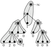
Figure 4: An illustration of the notions introduced in Definitions 4, 5, 6, and 7. Node labels indicate their height values. Circled nodes represent bad nodes. The dashed edge exists only in the extended configuration and connects the real root of the tree to the artificial node $\mathfrak{r}$. Each group of nodes is one component of the partition. The badness vector corresponding to this configuration is $(3,7,2,1,4)$.

We refer the reader to Figure 4 for an example of an extended configuration, its partition into components, and the corresponding badness vector.

Definition 8 (Lexicographic ordering)

Consider two badness vectors $\vec{b}=(x_{1},\dots,x_{k})$ and $\vec{b}^{\prime}=(x^{\prime}_{1},\dots,x^{\prime}_{k^{\prime}})$. We say that $\vec{b}^{\prime}$ is lexicographically smaller than $\vec{b}$ if one of the following holds:

1. $k^{\prime}<k$, or

2. $k^{\prime}=k$ and for some $i$ in the range $1\leq i\leq k$, $x^{\prime}_{i}<x_{i}$ and $x^{\prime}_{j}=x_{j}$ for all $j<i$.

The proof of the following lemma can be found in Appendix -E.

Lemma 9

If at least one bad node is activated or becomes non-bad in step $\mathcal{C}(t)\longrightarrow\mathcal{C}(t+1)$, then $\vec{b}(t+1)$ is lexicographically smaller than $\vec{b}(t)$.

Lemmas 8 and 9 are the essential ingredients required to prove convergence for the first phase. Appendix -F contains the full proof.

Theorem 10

In any execution, the first phase is completed in a finite number of steps.

V Simulation

To investigate the dynamic behavior and properties of our algorithm, we implemented a round based simulator. Each simulation ($i$) builds a full binary tree, ($ii$) initializes heights, and ($iii$) runs the balancing protocol. We used a synchronous daemon to run simulations, i.e., all the enabled nodes of the system execute their enabled actions simultaneously. The impact of non-deterministic daemons and/or the weaker daemon that is required to run our algorithm will be tackled in future work.

In the following, for a given simulation we will denote by $n$ the number nodes of the tree, by $h_{i}$ its initial height (i.e. after generation), by $h_{f}$ its final height (i.e. after balancing) and by $t$ the execution time in rounds.

V-A Almost Linear Trees

Intuitively, almost linear trees are stressing for a balancing algorithm because they are “as unbalanced as possible”. In the following, for a given $n$, the initial tree is the structurally unique full binary tree of height $\lceil n/2\rceil$. The only unspecified part of the simulation is the initial height values. It turns out that this has practically a very small impact on termination time. For each $n$ we ran thousands of simulations starting from the corresponding linear tree. For a given $n$ they always converged in the same number of rounds. As a consequence, all runs starting from the same linear tree will have approximately the same results.

Figure 5: $t$ for almost linear trees

Figure 6: $t$ for random trees

Figure 6 shows the termination time of simulations for different numbers of nodes. It contains two curves: the first one is plotted from our experiment and each point stands for an almost linear tree. The second curve is the sum of initial and final tree heights.

This plot tends to show that the round complexity of our algorithm is $\mathcal{}(n)$ in the worst case.

V-B Random Trees

To showcase the applicability of our algorithm to an existing system, trees are generated using the join protocol of [6].

Figure 6 shows the distance between the sum of initial and final tree heights and experimental termination times. The vertical axis gives the average variation between $h_{i}+h_{f}$ and experimental termination times. For each $n$ we ran thousands of simulations. Each candlestick sums up statistics on those runs; the whiskers indicates minimum and maximum variation, the cross indicates the average variation and the box height indicates the standard deviation.

The greater $n$ is, the closer $h_{i}+h_{f}$ and experimental results are. This result indicates that the average round complexity of our algorithm is $\mathcal{}(h_{i}+h_{f})$.

VI Concluding Remarks

In this work, we propose a new distributed self-stabilizing algorithm to rebalance containment-based trees using edge swapping. Simulation results indicate that the algorithm is quite efficient in terms of round complexity; in fact, it seems that we can reasonably expect $\mathcal{}(n)$ to be a worst-case bound, whereas in the average case the running time is closer to $\mathcal{}(h_{i}+h_{f})$ rounds. Interestingly, this average-case bound also appears in a different setting in [13]. Note that the conjectured average-case bound is close to $\mathcal{}(\log n)$ in a practically relevant scenario in which some faults appear (or new nodes are inserted) in an already balanced tree.

We have assumed that nodes keep correct copies of the height values of their children, so that each node can read the height values of its grandchildren by looking at the memory of its children. For simplicity, we have not dealt with the extra synchronization that would be required to maintain these copies up-to-date, but it should be possible to achieve this with a constant overhead per execution step. Furthermore, we have assumed that internal nodes have degree at least two. Degenerate internal nodes with degree one could be accommodated by a bottom-up protocol that runs in parallel and essentially disconnects them from the tree, attaching their children to their parents. Finally, note that in Section II we remarked that edge swaps may have semantic impact if they rearrange nodes so as to violate the containment relation. This can also be fixed by another bottom-up protocol that restores each node’s label to the minimum that suffices to contain the labels of its children.

Possible directions for future work include establishing the conjectured upper bounds of $\mathcal{}(n)$ and $\mathcal{}(h_{i}+h_{f})$ for the round complexity. We already have some preliminary results in this direction: the first phase of the algorithm (refer to Subsection IV-C) is indeed concluded in $\mathcal{}(n)$ rounds. An extension of this work would be to adapt the proposed algorithm in the message passing model.

-A Proof of Proposition 2

We prove that each node $u$ is balanced and has correct height information by induction on the actual height of $u$ in $\mathcal{C}(t^{\star})$.

If $h^{\star}_{u}(t^{\star})=0$, then $u$ is a leaf and since it is not enabled, $h_{u}(t^{\star})=0$. Therefore, $u$ has correct height information and is trivially balanced. Assume that all nodes of actual height $k$ or less, where $k\geq 0$, are balanced and have correct height information in $\mathcal{C}(t^{\star})$. Consider a node $u$ at actual height $k+1$. Since $u$ is not enabled for a height update, $h_{u}(t^{\star})=\max_{v\in\mathcal{S}_{u}(t^{\star})}h_{v}(t^{\star})+1$. But all children of $u$ are at actual height $k$ or less, therefore the inductive hypothesis and the last equality imply: $h_{u}(t^{\star})=\max_{v\in\mathcal{S}_{u}(t^{\star})}h^{\star}_{v}(t^{\star})+1=h^{\star}_{u}(t^{\star})$. Moreover, $u$ is not enabled for a swap, which means that for all children $v$ of $u$, $h_{v}(t^{\star})\geq h_{u}(t^{\star})-1-\alpha$, and because they have correct height information, $h^{\star}_{v}(t^{\star})\geq h^{\star}_{u}(t^{\star})-1-\alpha$. Therefore, $u$ has correct height information and is balanced.

-B Proof of Lemma 4

We will use the following notation in this section and in Appendices -D and -E. Let $P=\mathcal{C}\longrightarrow_{A}\mathcal{C}^{\prime}$ be a step of the execution. The set $A$ is partitioned into subsets $A_{h}$, $A_{b}$, and $A_{s}$, where $A_{h}$ is the set of non-bad nodes which perform a height update, $A_{b}$ is the set of bad nodes which perform a height update, and $A_{s}$ is the set of nodes which are sources of a swap. Let $A_{t}$ be the set of nodes which are targets of a swap and let $B$ and $B^{\prime}$ denote the set of bad nodes in configuration $\mathcal{C}$ and $\mathcal{C}^{\prime}$, respectively. For each node $u$, let $\mathcal{S}_{u}$ be the set of children of $u$ in $\mathcal{C}$ and $\mathcal{S}^{\star}_{u}$ be the set of nodes of the subtree rooted at $u$ in $\mathcal{C}$, and let $\mathcal{S}_{u}^{\prime}$ and ${\mathcal{S}^{\star}_{u}}^{\prime}$ be the corresponding sets in $\mathcal{C}^{\prime}$. Finally, let $\mathcal{G}(A_{b})$ be the subgraph induced by $A_{b}$ in the configuration $\mathcal{C}$.

The following lemma states some very basic properties that are easily derived from the definitions. It will be used implicitly throughout the proofs. We state it without proof.

Lemma 11 (Easy properties)

1. $A_{b}\subseteq B$.

2. $A_{s}\cap A_{h}=A_{s}\cap B=A_{t}\cap A_{h}=A_{t}\cap B=\emptyset$.

3. For all nodes $u$, $\mathcal{S}_{u}^{\prime}=\mathcal{S}_{u}$ if and only if $u\not\in A_{s}\cup A_{t}$.

4. The set of leaves in $\mathcal{C}^{\prime}$ is equal to the set of leaves in $\mathcal{C}$.

Lemma 12

Let $\mathcal{E}$ be a weakly connected component of $\mathcal{G}(A_{b})$. In $\mathcal{C}^{\prime}$, the nodes of $\mathcal{E}$ still induce a weakly connected subgraph which is identical to $\mathcal{E}$. No leaf of $\mathcal{E}$ belongs to $B^{\prime}$.

Proof:

No node of $\mathcal{E}$ is in $A_{s}\cup A_{t}$, therefore $\mathcal{S}_{v}^{\prime}=\mathcal{S}_{v}$ for all nodes $v$ of $\mathcal{E}$. This suffices to prove that the nodes of $\mathcal{E}$ induce in $\mathcal{C}^{\prime}$ a weakly connected subgraph that is identical to $\mathcal{E}$.

Now, let $u$ be a leaf of $\mathcal{E}$. If $u$ is also a leaf in $\mathcal{C}$, then its activation has set its height variable to $0$ in $\mathcal{C}^{\prime}$. But $u$ is still a leaf in $\mathcal{C}^{\prime}$, therefore it now has the correct height value and therefore $u\not\in B^{\prime}$. If $u$ is not a leaf of $\mathcal{C}$, it means that $\mathcal{S}_{u}$ is non-empty and $\mathcal{S}_{u}\cap A_{b}=\emptyset$ (if $v\in\mathcal{S}_{u}\cap A_{b}$, then $v$ would also be in $\mathcal{E}$ and $u$ would not be a leaf of $\mathcal{E}$). We deduce that each node in $\mathcal{S}_{u}$ either decreases or retains its height variable in $\mathcal{C}^{\prime}$. Moreover, by definition of the height update action, node $u$ adjusts its height variable to at least one greater than any of the values of the height variables of its children in $\mathcal{C}$. We conclude that $u\not\in B^{\prime}$. ∎

Lemma 13

If $u\not\in A\cup B$ and $\mathcal{S}_{u}^{\prime}\cap A_{b}=\emptyset$, then $u\not\in B^{\prime}$.

Proof:

Since $u$ is not activated, the value of its height variable remains the same in $\mathcal{C}^{\prime}$. Assume, first, that $u\not\in A_{t}$. Then, $\mathcal{S}_{u}^{\prime}=\mathcal{S}_{u}$ (since $u\not\in A_{s}$, either). Moreover, $\mathcal{S}_{u}^{\prime}\cap A_{b}=\emptyset$, therefore all nodes in $\mathcal{S}_{u}=\mathcal{S}_{u}^{\prime}$ either decreased or retained their height variables. From these observations and the fact that $u\not\in B$, we conclude that $u\not\in B^{\prime}$.

Now, assume that $u\in A_{t}$, and let $x\not\in A_{b}$ be its new child in $\mathcal{C}^{\prime}$. By the definition of the swap guard, the original height variable of node $x$ is strictly smaller than the height variable of $u$, and it may have decreased even further if $x$ was simultaneously activated for a height update. All other chilren of $u$ in $\mathcal{C}^{\prime}$ were also children of $u$ in $\mathcal{C}$, and, by the fact that $\mathcal{S}_{u}^{\prime}\cap A_{b}=\emptyset$, we know that they either decreased or retained their height values. From these observations and the fact that $u\not\in B$, we have that $u\not\in B^{\prime}$. ∎

Lemma 14

If $u\in A_{h}$ and $\mathcal{S}_{u}^{\prime}\cap A_{b}=\emptyset$, then $u\not\in B^{\prime}$.

Proof:

Since $u\in A_{h}$, we know that $u\not\in A_{s}\cup A_{t}$ and therefore $\mathcal{S}_{u}^{\prime}=\mathcal{S}_{u}$. Since $\mathcal{S}_{u}^{\prime}\cap A_{b}=\emptyset$, all its children either retain or decrease their height variable, whereas the height variable of $u$ is adjusted to at least one greater than any of the original values of the height variables of its children. Thus, $u\not\in B^{\prime}$. ∎

Lemma 15

If $u\in A_{s}$ and $\mathcal{S}_{u}^{\prime}\cap A_{b}=\emptyset$, then $u\not\in B^{\prime}$.

Proof:

Let $x\not\in A_{b}$ be the new child of $u$ in $\mathcal{C}^{\prime}$. By definition of the swap guard, we know that the height variable of $x$ in $\mathcal{C}^{\prime}$ is strictly smaller than that of $u$. All other children of $u$ were also children of $u$ in $\mathcal{C}$ and they have either retained or decreased their height variable, therefore $u\not\in B^{\prime}$. ∎

Lemma 16

$|B^{\prime}\setminus B|\leq|A_{b}\setminus B^{\prime}|$.

Proof:

To each node $x\in B^{\prime}\setminus B$, we associate a node $y\in A_{b}\setminus B^{\prime}$ as follows: By Lemmas 13, 14, and 15, a non-bad node $x$ in $\mathcal{C}$ can be turned into a bad node in $\mathcal{C}^{\prime}$ only if, in $\mathcal{C}^{\prime}$, it is the father of some node $b\in A_{b}$. In fact, this node $b$ must be the root of some weakly connected component $\mathcal{E}$ of $\mathcal{G}(A_{b})$: Otherwise, $b$ would have a father $u\in A_{b}$ in $\mathcal{C}$, and by Lemma 12, $u$ would still be the father of $b$ in $\mathcal{C}^{\prime}$, thus $u\equiv x$. This contradicts with the fact that $x\not\in B$. We define $y$ to be any leaf of $\mathcal{E}$, which, by Lemma 12, became non-bad in $\mathcal{C}^{\prime}$.

To conclude the argument, note that two distinct nodes $x,x^{\prime}\in B^{\prime}\setminus B$ must be the fathers of the roots of two distinct components of $\mathcal{G}(A_{b})$, and therefore they are associated to two distinct nodes $y$ and $y^{\prime}$. ∎

Lemma 17

$|B^{\prime}|\leq|B|$.

Proof:

One can easily verify that, for any sets $B$ and $B^{\prime}$, $|B^{\prime}|-|B|=|B^{\prime}\setminus B|-|B\setminus B^{\prime}|$. Since $A_{b}\subseteq B$, we have that $|A_{b}\setminus B^{\prime}|\leq|B\setminus B^{\prime}|$, therefore $|B^{\prime}|-|B|\leq|B^{\prime}\setminus B|-|A_{b}\setminus B^{\prime}|$. This, combined with Lemma 16, yields $|B^{\prime}|\leq|B|$. ∎

Lemma 4 follows immediately from Lemma 17.

-C Missing Proofs from Subsection IV-C1

Lemma 18

For any node $u$, if $h_{u}(t)<h^{\star}_{u}(t)$, then there exists in $\mathcal{C}(t)$ at least one bad node in the subtree rooted at $u$.

Proof:

By induction on the actual height of $u$. If $h^{\star}_{u}(t)=0$, then $u$ is a leaf and, by assumption, $h_{u}(t)<h^{\star}_{u}(t)=0$. Therefore, $u$ is a bad node. Now, assume that the statement holds for all nodes with actual height at most $k$, where $k\geq 0$. Consider a node $u$ with $h^{\star}_{u}(t)=k+1$ and let $v$ be one of its children with actual height $h^{\star}_{v}(t)=k$ (at least one such child must exist). We can assume that $u$ is not bad, otherwise the claim is proved. Since $u$ is not bad, $h_{v}(t)\leq h_{u}(t)-1$. By assumption, $h_{u}(t)\leq h^{\star}_{u}(t)-1$, thus we get $h_{v}(t)\leq h^{\star}_{u}(t)-2=k-1$. Since the actual height of $v$ is $k$, we have $h_{v}(t)<h^{\star}_{v}(t)$ and, by the inductive hypothesis, there exists a bad node in the subtree rooted at $v$. ∎

Lemma 19

In the second phase, if a node becomes enabled for a height update, it will remain enabled for a height update at least until it is activated.

Proof:

Note that a node that is enabled for a height update cannot be the source or the target of a swap, therefore its set of children does not change while it is enabled for a height update. Moreover, its children cannot increase their own height values, so the node will remain enabled for a height update at least until its activation. ∎

Proof:

Consider an execution of the algorithm in which an infinite number of height updates are executed. Since the number of nodes is finite, at least one node must execute a height update an infinite number of times. By the fact that the initial configuration contains no bad nodes and by Lemma 4, each time that node executes a height update, its height variable decreases. At some point, its height variable will become negative and at that point, by Lemma 18, some node in its subtree will become bad. This contradicts with Lemma 4. ∎

Proof:

By Lemma 5, there exists a finite time $t_{0}$ after which no height updates are performed. For each node $u$, let $h_{u}$ denote the value of its height variable at time $t_{0}$ and, since it remains constant thereafter, at all subsequent times. Furthermore, for $t\geq t_{0}$, let $\mathcal{\hat{S}}_{u}(t)$ denote the set of children of $u$ at time $t$ whose height variable is equal to $h_{u}-1$.

Note that $u$ is enabled for a height update at time $t$ if and only if $|\mathcal{\hat{S}}_{u}(t)|=0$. We observe now that in every step, if $u$ is the target of a swap then $|\mathcal{\hat{S}}_{u}(t)|$ is decreased by $1$, otherwise it remains the same. By Lemma 19, if $|\mathcal{\hat{S}}_{u}(t)|$ becomes $0$ then it remains equal to $0$ until $u$ performs a height update.

Suppose, now, for the sake of contradiction, that an infinite number of swaps are performed after time $t_{0}$. For each swap, there exists a node that is the target of that swap. It follows, then, that after at most $\sum_{u}|\mathcal{\hat{S}}_{u}(t_{0})|$ swaps have been performed after time $t_{0}$, all nodes in the system will be either idle or enabled for a height update (idle nodes will include nodes that are so low in the tree that they cannot possibly be the source of a swap and the root of the tree which will not be able to perform a swap since all of its children will be enabled for a height update). At that point, either all nodes are idle and thus the execution is completed, which contradicts with the fact that an infinite number of swaps are performed after time $t_{0}$, or the only choice of the scheduler is to activate a node for a height update, which contradicts with the fact that no height updates are performed after time $t_{0}$. ∎

-D Proof of Lemma 8

In this section, we use some notation introduced in Appendix -B. Additionally, in this section and in Appendix -E, we will use the following notation. Let $\tilde{\mathcal{C}}$ and $\tilde{\mathcal{C}}^{\prime}$ denote the extended configurations corresponding to $\mathcal{C}$ and $\mathcal{C}^{\prime}$, and let $\tilde{B}$ and $\tilde{B}^{\prime}$ denote the corresponding sets of bad nodes. Moreover, let $\{\mathcal{T}_{b}\}_{b\in B}$ and $\{\mathcal{T}^{\prime}_{b}\}_{b\in B^{\prime}}$ be the partition of nodes into components for the two configurations, and if $\mathcal{T}$ is any such component, let $V(\mathcal{T})$ denote its set of nodes.

Definition 9 (Swap chain)

A swap chain in step $P$ is a maximal-length directed path $u_{0},\dots,u_{\sigma}$ ($\sigma\geq 1$) in configuration $\mathcal{C}$ such that $u_{0},\dots,u_{\sigma-1}\in A_{s}$, $u_{1},\dots,u_{\sigma}\in A_{t}$, and, if $\sigma\geq 2$, $u_{2},\dots,u_{\sigma}$ are the swap-ins of the swaps performed by nodes $u_{0},\dots,u_{\sigma-2}$, respectively.

Lemma 20 (Properties of swap chains)

Let $u_{0},\dots,u_{\sigma}$ be a swap chain in step $P$.

1. $u_{1}\in\mathcal{S}_{u_{0}}^{\prime}$.

2. In $\mathcal{C}^{\prime}$, the nodes of even order in the swap chain ($u_{0},u_{2},\dots$) induce a directed path starting from $u_{0}$. Similarly, the nodes of odd order in the swap chain ($u_{1},u_{3},\dots$) induce a directed path starting from $u_{1}$.

3. $\bigcup_{i=0}^{\sigma}\mathcal{S}_{u_{i}}^{\prime}=\bigcup_{i=0}^{\sigma}\mathcal{S}_{u_{i}}$.

Proof:

Property 1 follows immediately from the fact that $u_{0}$ is the first node in the swap chain, therefore it is not the target of any swap operation. Property 2 follows from the fact that $u_{2},u_{4},\dots$ are the swap-in nodes for the swaps performed by nodes $u_{0},u_{2},\dots$ respectively and, similarly, $u_{3},u_{5},\dots$ are the swap-in nodes for the swaps performed by nodes $u_{1},u_{3},\dots$ respectively. For Property 3, note that the nodes in the swap chain exchange children only with other nodes in the swap chain. ∎

Lemma 21

If $u\not\in A_{t}$, then ${\mathcal{S}^{\star}_{u}}^{\prime}=\mathcal{S}^{\star}_{u}$.

Proof:

By induction on $|{\mathcal{S}^{\star}_{u}}^{\prime}|$. If $|{\mathcal{S}^{\star}_{u}}^{\prime}|=1$, then $u$ is a leaf in $\mathcal{C}^{\prime}$, thus also in $\mathcal{C}$, and ${\mathcal{S}^{\star}_{u}}^{\prime}=\mathcal{S}^{\star}_{u}=\{u\}$. Assume that the statement holds for all nodes whose subtree contains at most $k$ nodes in $\mathcal{C}^{\prime}$, where $k\geq 1$. Let $u\not\in A_{t}$ be a node for which $|{\mathcal{S}^{\star}_{u}}^{\prime}|=k+1$.

If $u\not\in A_{s}$, then $\mathcal{S}_{u}^{\prime}=\mathcal{S}_{u}$. Moreover, for all $z\in\mathcal{S}_{u}^{\prime}$, $|{\mathcal{S}^{\star}_{z}}^{\prime}|<|{\mathcal{S}^{\star}_{u}}^{\prime}|$ and $z\not\in A_{t}$, since their father was not the source of a swap. Therefore, the inductive hypothesis applies to each node $z\in\mathcal{S}_{u}^{\prime}$ and we get:

$${\mathcal{S}^{\star}_{u}}^{\prime}=\{u\}\cup\bigcup_{z\in\mathcal{S}_{u}^{\prime}}{\mathcal{S}^{\star}_{z}}^{\prime}=\{u\}\cup\bigcup_{z\in\mathcal{S}_{u}}\mathcal{S}^{\star}_{z}=\mathcal{S}^{\star}_{u}\enspace.$$

If $u\in A_{s}$, then $u$ must be the origin of a swap chain. Let $V_{\mathrm{ch}}$ be the node set of that swap chain and let $\mathcal{S}_{\mathrm{ch}}=\left(\bigcup_{v\in V_{\mathrm{ch}}}\mathcal{S}_{v}\right)\setminus V_{\mathrm{ch}}$ and $\mathcal{S}_{\mathrm{ch}}^{\prime}=\left(\bigcup_{v\in V_{\mathrm{ch}}}\mathcal{S}_{v}^{\prime}\right)\setminus V_{\mathrm{ch}}$. By Lemma 20, $\mathcal{S}_{\mathrm{ch}}^{\prime}=\mathcal{S}_{\mathrm{ch}}$. Moreover, each node $z\in\mathcal{S}_{\mathrm{ch}}^{\prime}$ is in the subtree of $u$ in $\mathcal{C}^{\prime}$ and $z\not\in A_{t}$. Therefore, the inductive hypothesis applies to each node $z\in\mathcal{S}_{\mathrm{ch}}^{\prime}$ and we get:

$${\mathcal{S}^{\star}_{u}}^{\prime}=V_{\mathrm{ch}}\cup\bigcup_{z\in\mathcal{S}_{\mathrm{ch}}^{\prime}}{\mathcal{S}^{\star}_{z}}^{\prime}=V_{\mathrm{ch}}\cup\bigcup_{z\in\mathcal{S}_{\mathrm{ch}}}\mathcal{S}^{\star}_{z}=\mathcal{S}^{\star}_{u}\enspace.$$

∎

Lemma 22

If $\tilde{B}^{\prime}=\tilde{B}$, then $V(\mathcal{T}^{\prime}_{b})=V(\mathcal{T}_{b})$, for all $b\in\tilde{B}$.

Proof:

Note that, for each $b\in\tilde{B}^{\prime}$, we can write $V(\mathcal{T}^{\prime}_{b})$ as follows:

$$V(\mathcal{T}^{\prime}_{b})={\mathcal{S}^{\star}_{b}}^{\prime}\setminus\bigcup_{u\in\tilde{B}^{\prime}\cap{\mathcal{S}^{\star}_{b}}^{\prime}\setminus\{b\}}{\mathcal{S}^{\star}_{u}}^{\prime}\enspace.$$

Since $b\in\tilde{B}^{\prime}=\tilde{B}$, we must have $b\not\in A_{t}$. Therefore, by Lemma 21, each $b\in\tilde{B}^{\prime}$ satisfies ${\mathcal{S}^{\star}_{b}}^{\prime}=\mathcal{S}^{\star}_{b}$. We get, then, that

$$V(\mathcal{T}^{\prime}_{b})={\mathcal{S}^{\star}_{b}}\setminus\bigcup_{u\in\tilde{B}\cap{\mathcal{S}^{\star}_{b}}\setminus\{b\}}{\mathcal{S}^{\star}_{u}}=V(\mathcal{T}_{b})\enspace.$$

∎

By Lemma 22, in a sequence of steps in which no bad node is activated or becomes non-bad, each of the connected components behaves in the same way as a tree that does not contain bad nodes. Therefore, by Lemmas 5 and 6, each component will stabilize in finite time and the bad nodes will be the only candidates for activation. Lemma 8 follows.

-E Proof of Lemma 9

In this section, we use some notation introduced in Appendices -B and -D. Additionally, in this section we will use the following notation. Let $\vec{b}$ and $\vec{b}^{\prime}$ denote the badness vectors corresponding to $\mathcal{C}$ and $\mathcal{C}^{\prime}$.

Lemma 23

If at least one bad node becomes non-bad without being activated in step $P$, then $|B^{\prime}|<|B|$.

Proof:

Let $N$ be the set of bad nodes that become non-bad without being activated. We can partition the set $B$ as follows:

$$B=N\cup\left(A_{b}\setminus B^{\prime}\right)\cup\left(B\cap B^{\prime}\right)\enspace.$$

Moreover, we can naturally partition the set $B^{\prime}$ as follows:

$$B^{\prime}=\left(B^{\prime}\setminus B\right)\cup\left(B\cap B^{\prime}\right)\enspace.$$

If $|N|>0$, then from the first equation we get $|B|>|A_{b}\setminus B^{\prime}|+|B\cap B^{\prime}|$, and then from the second equation and Lemma 16 we have that $|B^{\prime}|=|B^{\prime}\setminus B|+|B\cap B^{\prime}|\leq|A_{b}\setminus B^{\prime}|+|B\cap B^{\prime}|<|B|$. ∎

Lemma 24

If there exist nodes $u$ and $v$ such that $v\in\mathcal{S}_{u}^{\prime}\cap A_{b}$ and $u\in B\setminus A$ or $u\not\in B^{\prime}$, then $|B^{\prime}|<|B|$.

Proof:

We will prove the statement by demonstrating an injection from $B^{\prime}$ to $B\setminus\{v\}$. Consider the function $f:B^{\prime}\rightarrow B$ where, given $x\in B^{\prime}$, $f(x)$ is defined as follows:

• If $x\in B\setminus A_{b}$, then $f(x)=x$.

• Otherwise, $f(x)=y$ where $y$ is any child of $x$ in $\mathcal{C}^{\prime}$ such that $y\in A_{b}$.

We need to prove that the function $f$ is well-defined and injective. For injectivity, it suffices to show that if $x\not\in B\setminus A_{b}$, then $f(x)\not\in B\setminus A_{b}$. Indeed, given an $x\in B^{\prime}$ such that $x\not\in B\setminus A_{b}$, we distinguish two cases: If $x\not\in B$, then, by Lemmas 13, 14, and 15, $x$ has a child $y\in A_{b}$ in $\mathcal{C}^{\prime}$. On the other hand, if $x\in A_{b}$, then by Lemma 12 we know that $x$ is not a leaf of the component of $\mathcal{G}(A_{b})$ in which it belongs and thus it has a child $y\in A_{b}$ in $\mathcal{C}^{\prime}$. Clearly, in both cases, $y\not\in B\setminus A_{b}$.

It remains to show that no $x\in B^{\prime}$ is mapped to $v$. The only candidate nodes that could be mapped to $v$ are $v$ itself and $u$, the father of $v$ in $\mathcal{C}^{\prime}$. We know that $v\in A_{b}$, which implies that $v\not\in B\setminus A_{b}$, and thus $f(v)\neq v$. As for $u$, we have two cases: If $u\not\in B^{\prime}$, then $u$ is not even in the domain of $f$. If $u\in B^{\prime}$, then, by assumption, we must have $u\in B\setminus A$ and thus $f(u)=u\neq v$. ∎

For the proof of Lemma 9, we can assume that $\vec{b}^{\prime}$ and $\vec{b}$ are of equal length, otherwise the statement holds by Lemma 17. Moreover, we can assume that $A_{b}\neq\emptyset$, otherwise the statement holds by Lemma 23. Since $\mathfrak{r}\not\in A_{b}$, there exists a bad node in $\tilde{\mathcal{C}}$ whose corresponding component contains the parent of a node in $A_{b}$. Let $b_{j}$, $j\geq 1$, be the first such bad node in the ordering of Definition 7.

By definition of $b_{j}$, we have that $b_{1},\dots,b_{j}\not\in A_{b}$. Therefore, by Lemma 23, $b_{1},\dots,b_{j}\in\tilde{B}^{\prime}$. By Lemmas 13, 14, and 15, a non-bad node can be turned into a bad node only if, in $\tilde{\mathcal{C}}^{\prime}$, it is the father of a node in $A_{b}$. This implies that $b_{1},\dots,b_{j}$ are the first $j$ bad nodes in $\tilde{\mathcal{C}}^{\prime}$ according to the ordering of Definition 7.

By definition of $b_{j}$ and Lemma 23, we also know that any child of any node in any of the components $\mathcal{T}_{b_{1}},\dots,\mathcal{T}_{b_{j-1}}$, that was in $\tilde{B}$, is also in $\tilde{B}^{\prime}$. Therefore, for each $i<j$, $|\mathcal{T}^{\prime}_{b_{i}}|=|\mathcal{T}_{b_{i}}|$. Finally, by Lemma 24, we can assume that $b_{j}$ itself is not the father of any node $v\in A_{b}$ and that, for any such node $v$ whose father $w$ was in $\mathcal{T}_{b_{j}}$, at least $w$ no longer belongs to $\mathcal{T}^{\prime}_{b_{j}}$. Therefore, $|\mathcal{T}^{\prime}_{b_{j}}|<|\mathcal{T}_{b_{j}}|$.

-F Proof of Theorem 10

By Lemma 9, the badness vector decreases lexicographically whenever at least one bad node is activated or becomes non-bad. By Lemma 8, we cannot have an infinite sequence of steps in which no bad node is activated or becomes non-bad. Moreover, during such a sequence of steps, the set of bad nodes remains the same by Lemmas 13, 14, and 15, and thus the badness vector remains the same by Lemma 22. The theorem follows from these observations and the easy fact that no configuration can have a corresponding badness vector that is lexicographically smaller than the single-component badness vector $(n+1)$, where $n$ is the number of nodes in the system.

References

- [1] R. Bayer and E. McCreight, “Organization and maintenance of large ordered indices,” in Acta Informatica 1, 1972, pp. 173–189.
- [2] A. Guttman, “R-trees: a dynamic index structure for spatial searching,” in ACM SIGMOD, 1984, pp. 47–57.
- [3] P. Ciaccia, M. Patella, and P. Zezula, “M-tree: An efficient access method for similarity search in metric spaces,” in VLDB, 1997, pp. 426–435.
- [4] S. Bianchi, A. K. Datta, P. Felber, and M. Gradinariu, “Stabilizing peer-to-peer spatial filters,” in ICDCS 2007, 2007, p. 27.
- [5] H. V. Jagadish, B. C. Ooi, Q. H. Vu, R. Zhang, and A. Zhou, “Vbi-tree: A peer-to-peer framework for supporting multi-dimensional indexing schemes,” in ICDE, 2006, p. 34.
- [6] T. Izumi, M. G. Potop-Butucaru, and M. Valero, “Physical expander in virtual tree overlay,” in DISC, 2011, pp. 82–96.
- [7] W. Edsger and Dijkstra., “Self-stabilizing systems in spite of distributed control,” Commum. ACM, vol. 17, no. 11, pp. 643–644, 1974.
- [8] C. du Mouza, W. Litwin, and P. Rigaux, “SD-Rtree: A scalable distributed rtree,” Data Engineering, International Conference on, vol. 0, pp. 296–305, 2007.
- [9] Adelson-Velskii and Landis, “An algorithm for the organization of information,” in Proceedings of the USSR Academy of Sciences, 1962.
- [10] H. V. Jagadish, B. C. Ooi, and Q. H. Vu, “Baton: a balanced tree structure for peer-to-peer networks,” in VLDB, 2005, pp. 661–672.
- [11] T. Herman and T. Masuzawa, “Available stabilizing heaps,” Information Processing Letters, vol. 77, pp. 115–121, 2001.
- [12] D. Bein, A. Datta, and V. Villain, “Snap-stabilizing optimal binary search tree,” in Seventh International Symposium on Self-Stabilizing Systems (SSS’05). Barcelona, Spain: LNCS 3764, 2005, pp. 1–17.
- [13] E. Caron, F. Desprez, F. Petit, and C. Tedeschi, “Snap-stabilizing prefix tree for peer-to-peer systems,” Parallel Processing Letters, vol. 20, no. 1, pp. 15–30, March 2010.
- [14] F. Luccio and L. Pagli, “On the height of height-balanced trees,” IEEE Trans. Computers, vol. 25, no. 1, pp. 87–91, 1976.
- [15] T. H. Cormen, C. E. Leiserson, R. L. Rivest, and C. Stein, Introduction to Algorithms, Second Edition. The MIT Press, 2001.
- [16] J. Burns, M. Gouda, and R. Miller, “On relaxing interleaving assumptions,” in Proceedings of the MCC Workshop on Self-Stabilizing Systems, MCC Technical Report No. STP-379-89, 1989.