Approximating rational Bézier curves by constrained Bézier curves of arbitrary degree

Abstract

In this paper, we propose a method to obtain a constrained approximation of a rational Bézier curve by a polynomial Bézier curve. This problem is reformulated as an approximation problem between two polynomial Bézier curves based on weighted least-squares method, where weight functions $\rho(t)=\omega(t)$ and $\rho(t)=\omega(t)^{2}$ are studied respectively. The efficiency of the proposed method is tested using some examples.

AMS 2000 Subject Classifications: 41A10.41A25.65D10.65D17.

1 Introduction

Rational Bézier curves play a significant role in Computer Aided Design systems. However, the forms of derivatives are quite complex and integral expressions may not exist for high-degree rational Bézier curves, so the problem of approximating rational functions with polynomials has been raised and studied. Sederberg and Kakimoto [1] presented the hybrid polynomial approximation to rational curves for the first time in 1991. Wang et al.[2][3] presented Hermite polynomial approximations to rational Bézier curves and investigated the convergence condition for the polynomial approximation of rational functions and rational curves. Floater [4] constructed a high-order approximation of rational curves using polynomial curves. Lee [5] converted a polynomial approximation of a rational Bézier curve to control points approximation of two Bézier curves. An approximate solution was obtained by least-squares method. Huang [6] presented a simple method for approximating a rational Bézier curve with a Bézier curve sequence based on degree elevation. Recently, sample-based polynomial approximation of rational Bézier curves was investigated by Lu [7], whose errors smaller than Huang’s. Hu [8] proposed a reparameterization-based method for polynomial approximating rational Bézier curves with constraints.

In this paper, we propose a method to obtain a constrained approximation of a rational Bézier curve by a polynomial Bézier curve based on weighted least-squares [9]. The main idea is converting a polynomial approximation of a rational Bézier curve to an approximation between two Bézier curves so that control points of a Bézier curve can be obtained using linear equations. Compared with the related works in paper [5] , [7] and [8], our method is fast, stable and highly accurate to obtain some higher degree Bézier curves as well as don’t need fix parameter $\lambda$.

The paper is structured as follows. Section 2 presents some basic concepts and properties regarding the problem of the constrained Bézier approximation of a rational Bézier curve. Section 3 brings a complete solution to the problem formulated above in the $L_{2}$ norm. Section 4 presents some numerical examples to verify the accuracy and effectiveness of the method.

2 Preliminaries

2.1 Definitions and Properties

A standard-form $n$th degree rational Bézier curve is defined as follows [10]:

$$\textit{{P}}(t)=\frac{\textbf{{x}}(t)}{\omega(t)}=\frac{\sum\limits_{i=0}^{n}\omega_{i}\textit{{p}}_{i}B_{i}^{n}(t)}{\sum\limits_{i=0}^{n}\omega_{i}B_{i}^{n}(t)},\ t\in[0,1],$$ (1)

where $B_{i}^{n}(t)={n\choose i}t^{i}(1-t)^{n-i}$ are the Bernstein polynomials, $\textit{{p}}_{i}\in\mathbb{R}^{d},i=0,1,...,n,$ are control points, and $\omega_{i}\in\mathbb{R}^{+},i=0,1,...,n,\omega_{0}=\omega_{n}=1$, are the scalar weights. Clearly, polynomial function $\omega(t)>0$.

The following are pertinent theorems used in this paper:

Theorem 1.

The product of degree $m$ Bernstein polynomials and its integral satisfies

$$\prod_{j=1}^{m}B_{i_{j}}^{n_{j}}(t)=\frac{{M}}{{N\choose J}}B_{J}^{N}(t),$$ (2)

$$\int_{0}^{1}\prod_{j=1}^{m}B_{i_{j}}^{n_{j}}(t)dt=\frac{M}{(N+1){N\choose J}},$$ (3)

where $M=\prod_{j=1}^{m}{n_{j}\choose i_{j}}$, $N=\sum_{j=1}^{m}n_{j}$ and $J=\sum_{j=1}^{m}i_{j}$.

Theorem 2.

Let the two polynomials $f(t)$ and $g(t)$ of degree $m$ and $n$ with coefficients $f_{i}^{m}$ and $g_{i}^{n}$ be as follows

$$f(t)=\sum_{i=a}^{k}f_{i}^{m}B_{i}^{m}(t),\ \ g(t)=\sum_{i=0}^{n}g_{i}^{n}B_{i}^{n}(t),$$

where $0\leq a<k\leq m$. Their product is a degree $m+n$ polynomial

$$f(t)g(t)=\sum_{i=a}^{k+n}\left(\sum_{j=max(a,i-n)}^{min(k,i)}\frac{{m\choose j}{n\choose i-j}}{{m+n\choose i}}f_{j}^{m}g_{i-j}^{n}\right)B_{i}^{m+n}(t).$$ (4)

Theorem 3.

For each appropriate function $f(x)\in C_{[a,b]}$, there is a unique polynomial $P_{n}(x)$ of degree at most $n$ to approximate $f(x)$, such that $\int_{a}^{b}(f(x)-P_{n}(x))^{2}dx$ is minimum ([9]).

2.2 Statement of the approximation problem

The problem of approximating rational Bézier curves in equation (1) by constrained Bézier curves of arbitrary degree is that of finding control points $\textbf{{q}}_{0},\textbf{{q}}_{1},...,\textbf{{q}}_{m}$, which define a Bézier curve of degree $m$

$$\textbf{Q}(t)=\sum\limits_{i=0}^{m}B_{i}^{m}(t)\textit{{q}}_{i},$$ (5)

such that the following two conditions are satisfied simultaneously:

1) Bézier curve $\textbf{Q}(t)$ has the contact order $(k,h)\ (k,h=0,1,2)$ of continuity at both endpoints of the rational Bézier curve $\textbf{{P}}(t)$.

2) Given a weight function $\rho(t)>0$, a distance function $d_{\rho}(\textbf{{P}},\textit{{Q}})$ between $\textbf{{P}}(t)$ and $\textbf{{Q}}(t)$ in the $L_{2}$ norm is minimized, that is

$$\begin{split}d_{\rho}(\textbf{{P}},\textbf{{Q}})&=\int_{0}^{1}\rho(t)\left(\textbf{{P}}(t)-\textbf{{Q}}(t)\right)^{2}dt.\\ &=\int_{0}^{1}\frac{\rho(t)}{\omega^{2}(t)}\left(\textbf{{x}}(t)-\omega(t)\textbf{{Q}}(t)\right)^{2}dt,\end{split}$$

and the control points $\textit{{q}}_{l}(l=k+1,k+2,...,m-h-1)$ of $\textbf{Q}(t)$ satisfy

$$\frac{\partial d_{\rho}(\textit{{P}},\textit{{Q}})}{\partial\textit{{q}}_{l}}=2\int_{0}^{1}\left(\textbf{{x}}(t)-\omega(t)\textbf{{Q}}(t)\right)B_{l}^{m}(t)\frac{\rho(t)}{\omega(t)}dt=0.$$ (6)

Clearly, in this paper the function $\omega(t)$ is a factor of function $\rho(t)$.

In this paper,we shall study constrained polynomials approximation in the next section. For simplicity, assume that $\rho(t)=\omega(t)$ and $\rho(t)=\omega^{2}(t)$ respectively.

3 Algorithm for constrained Bézier approximation

The approximation algorithm is completed through a two-step process. First, we calculate the constrained control points of the approximation Bézier curve $\textbf{{Q}}(t)$ by imposing the contact order in the condition 1). Next, we calculate other unconstrained control points by using the weighted least-squares method, in order to satisfy condition 2).

3.1 Constrained conditions of the approximation curve

According to equation (1), we have

$$\textbf{{x}}(t)=\textbf{{P}}(t)\omega(t).$$

Taking the derivative of the above equation $r(=0,1,2)$ times, we obtain

$$\textbf{{x}}^{(r)}(t)=\sum\limits_{j=0}^{r}{r\choose j}\omega^{(j)}(t)\textbf{{P}}^{(r-j)}(t).$$

Thus, we have the zero, first and second derivatives of $\textbf{{P}}(t)$ at two endpoints $(t=0,1)$, satisfying the following, respectively

$$\begin{split}\textit{{P}}(0)&=\textit{{p}}_{0},\ \textbf{{P}}(1)=\textbf{{p}}_{n},\\ \textit{{P}}\ ^{\prime}(0)&=n\omega_{1}(\textbf{{p}}_{1}-\textbf{{p}}_{0}),\ \textit{{P}}\ ^{\prime}(1)=n\omega_{n-1}(\textbf{{p}}_{n}-\textbf{{p}}_{n-1}),\\ \textit{{P}}\ ^{\prime\prime}(0)&=n\left\{\omega_{2}(n-1)\textbf{{p}}_{2}+2\omega_{1}(1-n\omega_{1})\textbf{{p}}_{1}+[2\omega_{1}(n\omega_{1}-1)+\omega_{2}(1-n)]\textbf{{p}}_{0}\right\},\\ \textit{{P}}\ ^{\prime\prime}(1)&=n\{[2\omega_{n-1}(n\omega_{n-1}-1)+\omega_{n-2}(1-n)]\textbf{{p}}_{n}+2\omega_{n-1}(1-n\omega_{n-1})\textbf{{p}}_{n-1}\\ &+(n-1)\omega_{n-1}\textbf{{p}}_{n-2}\}.\end{split}$$

Since the zero, first and second derivatives of $\textbf{{Q}}(t)$ at two endpoints $(t=0,1)$ can be described as

$$\begin{split}\textit{{Q}}(0)&=\textit{{q}}_{0},\ \textbf{{Q}}(1)=\textbf{{q}}_{m},\\ \textit{{Q}}\ ^{\prime}(0)&=m(\textbf{{q}}_{1}-\textbf{{q}}_{0}),\ \textit{{Q}}\ ^{\prime}(1)=m(\textbf{{q}}_{m}-\textbf{{q}}_{m-1}),\\ \textit{{Q}}\ ^{\prime\prime}(0)&=m(m-1)(\textbf{{q}}_{2}-2\textbf{{q}}_{1}+\textbf{{q}}_{0}),\\ \textit{{Q}}\ ^{\prime\prime}(1)&=m(m-1)(\textbf{{q}}_{m}-2\textbf{{q}}_{m-1}+\textbf{{q}}_{m-2}),\end{split}$$

matching the function value and derivatives up to the second order at both endpoints of $\textbf{{P}}(t)$ and $\textbf{{Q}}(t)$, the constrained control points of $\textbf{{Q}}(t)$ are

$$\textbf{{q}}_{0} =\textbf{{p}}_{0},\textbf{{q}}_{m}=\textit{{p}}_{n},$$

$$\textrm{if}\ m\geq 2,\ \ \ \ \textbf{{q}}_{1} =\frac{n}{m}\omega_{1}\textbf{{p}}_{1}+\left(1-\frac{n}{m}\omega_{1}\right)\textbf{{p}}_{0},$$

$$\textrm{if}\ m\geq 3,\textbf{{q}}_{m-1} =\left(1-\frac{n}{m}\omega_{n-1}\right)\textbf{{p}}_{n}+\frac{n}{m}\omega_{n-1}\textbf{{p}}_{n-1},$$

$$\textrm{if}\ m\geq 4,\ \ \ \ \textbf{{q}}_{2} =\frac{1}{m(m-1)}\{n(n-1)\omega_{2}\textbf{{p}}_{2}+2n\omega_{1}(m-n\omega_{1})\textbf{{p}}_{1}$$

$$+[m(m-1)+2n\omega_{1}(n\omega_{1}-m)+n\omega_{2}(1-n)]\textbf{{p}}_{0}\},$$

$$\textrm{if}\ m\geq 5,\textbf{{q}}_{m-2} =\frac{1}{m(m-1)}\{[2n\omega_{n-1}(n\omega_{n-1}-m)+n\omega_{n-2}(1-n)+m(m-1)]\textbf{{p}}_{n}$$

$$+{2n\omega_{n-1}}(m-n\omega_{n-1})\textbf{{p}}_{n-1}+{n(n-1)}\omega_{n-2}\textbf{{p}}_{n-2}\}.$$

Accordingly, Q(t) can be rewritten as

$$\textbf{{Q}}(t)=\sum\limits_{i=0}^{k}B_{i}^{m}(t)\textbf{{q}}_{i}+\sum\limits_{i=k+1}^{m-h-1}B_{i}^{m}(t)\textbf{{q}}_{i}+\sum\limits_{i=m-h}^{m}B_{i}^{m}(t)\textit{{q}}_{i},$$ (7)

where $\textbf{{q}}_{i}(i=k+1,k+2,...,m-h-1)$ are the unknown control points and

$$k=\begin{cases}0&m=1,\\ 1&m=2,3,\\ 2&m\geq 4,\end{cases}\ \ h=\begin{cases}0&m=1,2,\\ 1&m=3,4,\\ 2&m\geq 5.\end{cases}$$

3.2 Unconstrained control points of the approximation curve

3.2.1 $\rho(t)=\omega(t)$

When $\rho(t)=\omega(t)$, based on equation (6) we have

$$\int_{0}^{1}\textbf{{Q}}(t)\omega(t)B_{l}^{m}(t)dt=\int_{0}^{1}\textbf{{x}}(t)B_{l}^{m}(t)dt.$$ (8)

Substituting (7) into (8), we get

$$\sum\limits_{i=0}^{k}\int_{0}^{1}\omega(t)B_{i}^{m}(t)B_{l}^{m}(t)\textbf{{q}}_{i}dt+\sum\limits_{i=k+1}^{m-h-1}\int_{0}^{1}\omega(t)B_{i}^{m}(t)B_{l}^{m}(t)\textbf{{q}}_{i}dt$$ (9)

$$+\sum\limits_{i=m-h}^{m}\int_{0}^{1}\omega(t)B_{i}^{m}(t)B_{l}^{m}(t)\textbf{{q}}_{i}dt=\int_{0}^{1}\textbf{{x}}(t)B_{l}^{m}(t)dt.$$

By deriving equation (9) based on theorems 1 and 2, we obtain

$$\sum\limits_{i=0}^{n+k}\left(\sum\limits_{j=max(0,i-n)}^{min(k,i)}\frac{{m\choose j}{n\choose i-j}}{{2m+n\choose i+l}}\omega_{i-j}\textbf{{q}}_{j}\right)+\sum\limits_{i=k+1}^{n+m-h-1}\left(\sum\limits_{j=max(k+1,i-n)}^{min(m-h-1,i)}\frac{{m\choose j}{n\choose i-j}}{{2m+n\choose i+l}}\omega_{i-j}\textbf{{q}}_{j}\right)$$

$$+\sum\limits_{i=m-h}^{n+m}\left(\sum\limits_{j=max(m-h,i-n)}^{min(m,i)}\frac{{m\choose j}{n\choose i-j}}{{2m+n\choose i+l}}\omega_{i-j}\textbf{{q}}_{j}\right)$$

$$=\frac{2m+n+1}{m+n+1}\sum\limits_{i=0}^{n}\left(\frac{{n\choose i}}{{n+m\choose i+l}}\omega_{i}\textbf{{p}}_{i}\right),$$

$$(l=k+1,k+2,...,m-h-1).$$ (10)

To easily evaluate the unknown points $\textit{{q}}_{i}(i=k+1,k+2,...,m-h-1)$, we rearrange equation (10) to obtain

$$\sum\limits_{i=k+1}^{m-h-1}\sum\limits_{j=0}^{n}\frac{{n\choose j}{m\choose i}}{{2m+n\choose i+j+l}}\omega_{j}\textbf{{q}}_{i}=\frac{2m+n+1}{m+n+1}\sum\limits_{i=0}^{n}\frac{{n\choose i}}{{m+n\choose i+l}}\omega_{i}\textbf{{p}}_{i}$$

$$-\sum\limits_{i=0}^{k}\sum\limits_{j=0}^{n}\frac{{n\choose j}{m\choose i}}{{2m+n\choose i+j+l}}\omega_{j}\textbf{{q}}_{i}-\sum\limits_{i=m-h}^{m}\sum\limits_{j=0}^{n}\frac{{n\choose j}{m\choose i}}{{2m+n\choose i+j+l}}\omega_{j}\textbf{{q}}_{i},$$ (11)

$(l=k+1,k+2,...,m-h-1).$

3.2.2 $\rho(t)=\omega(t)^{2}$

When $\rho(t)=\omega(t)^{2}$, one has

$$\int_{0}^{1}\textbf{{Q}}(t)\omega^{2}(t)B_{l}^{m}(t)dt=\int_{0}^{1}\textbf{{x}}(t)\omega(t)B_{l}^{m}(t)dt.$$ (12)

Substituting (7) into (12), it yields

$$\sum\limits_{i=0}^{k}\int_{0}^{1}\omega^{2}(t)B_{i}^{m}(t)B_{l}^{m}(t)\textbf{{q}}_{i}dt+\sum\limits_{i=k+1}^{m-h-1}\int_{0}^{1}\omega^{2}(t)B_{i}^{m}(t)B_{l}^{m}(t)\textbf{{q}}_{i}dt$$ (13)

$$+\sum\limits_{i=m-h}^{m}\int_{0}^{1}\omega^{2}(t)B_{i}^{m}(t)B_{l}^{m}(t)\textbf{{q}}_{i}dt=\int_{0}^{1}\textbf{{x}}(t)\omega(t)B_{l}^{m}(t)dt.$$

By deriving equation (13) based on theorems 1 and 2, we obtain

$$\sum\limits_{i=0}^{2n+k}\left(\sum\limits_{j=max(0,i-2n)}^{min(k,i)}\frac{{m\choose j}{2n\choose i-j}}{{2m+2n\choose i+l}}W_{i-j}\textbf{{q}}_{j}\right)+\sum\limits_{i=k+1}^{2n+m-h-1}\left(\sum\limits_{j=max(k+1,i-2n)}^{min(m-h-1,i)}\frac{{m\choose j}{2n\choose i-j}}{{2m+2n\choose i+l}}W_{i-j}\textbf{{q}}_{j}\right)$$

$$+\sum\limits_{i=m-h}^{2n+m}\left(\sum\limits_{j=max(m-h,i-2n)}^{min(m,i)}\frac{{m\choose j}{2n\choose i-j}}{{2m+2n\choose i+l}}W_{i-j}\textbf{{q}}_{j}\right)$$

$$=\frac{2m+2n+1}{m+2n+1}\sum\limits_{i=0}^{2n}\left(\sum\limits_{j=max(0,i-n)}^{min(n,i)}\frac{{n\choose j}{n\choose i-j}}{{2n+m\choose i+l}}\omega_{i-j}\omega_{j}\textbf{{p}}_{j}\right),$$

$$(l=k+1,k+2,...,m-h-1),$$ (14)

where

$$W_{i}=\sum\limits_{j=max(0,i-n)}^{min(n,i)}\frac{{n\choose j}{n\choose i-j}}{{2n\choose i}}\omega_{i-j}\omega_{j}.$$

We rearrange equation (14) to obtain

$$\sum\limits_{i=k+1}^{m-h-1}\sum\limits_{j=0}^{2n}\frac{{2n\choose j}{m\choose i}}{{2n+2m\choose i+j+l}}W_{j}\textbf{{q}}_{i}=\frac{2m+2n+1}{2m+n+1}\sum\limits_{i=0}^{n}\sum\limits_{j=0}^{n}\frac{{n\choose i}{n\choose j}}{{2n+m\choose i+j+l}}\omega_{i}\omega_{j}\textbf{{p}}_{i}$$

$$-\sum\limits_{i=0}^{k}\sum\limits_{j=0}^{2n}\frac{{2n\choose j}{m\choose i}}{{2n+2m\choose i+j+l}}W_{j}\textbf{{q}}_{i}-\sum\limits_{i=m-h}^{m}\sum\limits_{j=0}^{2n}\frac{{2n\choose j}{m\choose i}}{{2n+2m\choose i+j+l}}W_{j}\textbf{{q}}_{i},$$ (15)

$(l=k+1,k+2,...,m-h-1).$

Finally, by theorem 3, we conclude that the solution of linear system (11) and (15) is unique. They can be obtained by any methods introduced in [9].

4 Error estimation and implementation

Since

$$d_{\rho}(\textbf{{P}},\textbf{{Q}}) =\left(\int_{0}^{1}\rho(t)\left|\textbf{{P}}(t)-\textbf{{Q}}(t)\right|^{p}dt\right)^{\frac{1}{p}}$$ (16)

$$\leq\left(\int_{0}^{1}\rho(t)dt\right)^{\frac{1}{p}}\left(\max\limits_{0\leq t\leq 1}\left\|\textbf{{P}}(t)-\textbf{{Q}}(t)\right\|\right),$$

we use maximum distance $d_{max}$ to evaluate the approximation results for the convenience of estimation. More specifically, by dividing $[0,1]$ into H subintervals of equal length $h=\frac{1}{H}$, it allows

$$d_{max}=\max\limits_{0\leq i\leq H}\|\textit{{P}}(t_{i})-\textbf{{Q}}(t_{i})\|,$$

where $t_{i}=ih\ (i=0,1,...,H)$ are evenly spaced values in the parameter domain $[0,1]$.

Another error for the approximation used here was given by Lu [7]. That is

$$d_{l_{1}}(\textbf{{P}},\textbf{{Q}})=\frac{h}{2}\sum_{i=0}^{H-1}(\|\textbf{{P}}(t_{i})-\textbf{{Q}}(t_{i})\|+\|\textbf{{P}}(t_{i+1})-\textbf{{Q}}(t_{i+1})\|).$$

Obviously, $d_{max}>d_{l_{1}}$ by Equation (16). Finally, for more details about error analysis of weighted least-squares we refer the reader to [11].
There is a disadvantage for approximating rational Bézier curve by Bézier curve: when an original rational Bézier curve is convex, but the resulting Bézier curve may be non-convex. To deal with this problem, we use higher degree Bézier curve to reduce the approximation error (see Example 3).

Example 1. A rational Bézier curve of degree 3 is defined by the control points (0, 0), (0.2, 1.5), (0.8, 1.5), (1,0) and the associated weights 1, 1.2, 1.5, 1. Table 1. lists the errors obtained by the weighted least-squares and the Lee’s method in [5] for $n=4,5,6,7,8,$ respectively. From the comparison of the errors , our algorithm can mostly produce better approximation results than Lee’s method.

Table 1: Errors approximation to the rational Bézier curve of degree 3

$n$	maximum error				$L_{1}$-error
	$\rho=\omega(t)$	$\rho=\omega^{2}(t)$	Lee’s method		$\rho=\omega(t)$	$\rho=\omega^{2}(t)$	Lee’s method
			The 1st	The 2nd			The 1st	The 2nd
			method (r=100)	method			method(r=100)	method
4	0.022907	0.023911	0.020312	0.053134	0.004237	0.004185	0.004679	0.004295
5	0.007390	0.007743	0.006150	0.024009	0.001162	0.001149	0.002205	0.001424
6	0.002849	0.002987	0.004098	0.011423	4.371940e-04	4.321077e-04	0.002058	6.297696e-04
7	8.065401e-04	8.469361e-04	0.003461	0.004955	1.057862e-04	1.045051e-04	0.002046	2.004255e-04
8	2.870556e-04	3.017434e-04	0.003400	0.002312	3.871330e-05	3.827086e-05	0.002030	9.057967e-05

Example 2 (Also Example 1 in [7]). A rational Bézier curve of degree 7 is defined by the control points (0, 0), (0.5, 2), (1.5, 2), (2.5, .2), (3.5,.2), (4.5, 2), (5.5, 2), (6, 0) and the associated weights 1, 2, 1/3, 2, 2, 1/3, 2, 1. Table 2. lists the errors obtained by the weighted least-squares and the Lu’s method in [7] for $n=5,6,...,18,$ respectively. By comparison for $L_{1}$ error , our algorithm can produce better approximation results than Lu’s method as $n=7,8,...,18$. However, for maximum error, we find that $\rho(t)=\omega(t)$ method generated smaller error values than $\rho(t)=\omega^{2}(t)$ method, but it is reverse for $L_{1}$ error.

Table 2: Errors approximation to the rational Bézier curve of degree 7

$n$	maximum error		$L_{1}$-error
	$\rho=\omega(t)$	$\rho=\omega^{2}(t)$	$\rho=\omega(t)$	$\rho=\omega^{2}(t)$	Lu’s method ($\lambda$=0.95)[7]
5	0.095480	0.097236	0.049830	0.049584	0.043439
6	0.084855	0.086855	0.047010	0.046837	0.040826
7	0.042564	0.043096	0.011913	0.011892	0.037923
8	0.035610	0.037288	0.012254	0.012140	0.035547
9	0.035619	0.037298	0.012246	0.012133	0.023335
10	0.005224	0.005420	0.001600	0.001578	0.016259
11	0.005374	0.005620	0.001566	0.001537	0.013806
12	0.003154	0.003335	9.999698e-04	9.814476e-04	0.012295
13	0.002257	0.002361	3.797283e-04	3.675078e-04	0.011220
14	0.001222	0.001307	2.998330e-04	2.944257e-04	0.009933
15	0.001206	0.001290	2.802343e-04	2.754957e-04	0.008897
16	2.834610e-04	3.006113e-04	5.642958e-05	5.503411e-05	0.006065
17	2.687450e-04	2.860145e-04	5.593685e-05	5.458823e-05	0.002309
18	1.240139e-04	1.326072e-04	2.950490e-05	2.879857e-05	0.001462

Example 3. Consider a 4th-degree rational Bézier curve P(t) with control points (0, 0), (0.2, 1.5),(0.5, 1.0), (0.8, 1.5), (1, 0) and the associated weights 1, 0.06, 0.08, 0.05, 1. The $n$th-degree, $n=6,7,...,23$, Bézier curves $\textbf{{Q}}(t)$ approximating $\textbf{{P}}(t)$ with the contact order $(1,1)$ of continuity at two endpoints. Table 3. lists the error obtained by $\rho(t)=\omega(t)$ and $\rho(t)=\omega^{2}(t)$ for $n=6,7,...,25$, respectively. For both maximum error and $L_{1}$ error, we find that $\rho(t)=\omega(t)$ method generated smaller error values than $\rho(t)=\omega^{2}(t)$ method. Fig 1. shows that the resulting $C^{(1,1)}$-continuity approximation curve of degree 6 is nonconvex at near zero. Fig 2. shows that the given curve and the resulting curve of degree 18 are almost the same.

Table 3: Errors approximation to the rational Bézier curve of degree 4

$n$	maximum error		$L_{1}$-error
	$\rho=\omega(t)$	$\rho=\omega^{2}(t)$	$\rho=\omega(t)$	$\rho=\omega^{2}(t)$
6	0.044480318880273	0.051688479122085	0.029655280096461	0.031476147607478
7	0.023868501893973	0.032255328068047	0.015879504757276	0.017049959327487
8	0.015149900429568	0.018966490675292	0.009620768974042	0.010354259252695
9	0.007889349654775	0.010828999111530	0.005297861401833	0.005727317319065
10	0.005260808682043	0.006853089108748	0.003256996716366	0.003527894117667
11	0.002696794398629	0.003727944822126	0.001818736806966	0.001974652524091
12	0.001847253697888	0.002461821331414	0.001126845692919	0.001225098891989
13	9.389817537108827e-04	0.001303331966052	6.345106044598648e-04	6.908760850927994e-04
14	6.534387865426517e-04	8.830834863300054e-04	3.949335561005876e-04	4.303886131207782e-04
15	3.306456957305267e-04	4.601136641000896e-04	2.236082280218562e-04	2.439441476699068e-04
16	2.323377554374534e-04	3.169111231735876e-04	1.395669996426054e-04	1.523518332243233e-04
17	1.172969349325125e-04	1.635210281226485e-04	7.933336636596293e-05	8.667628246221323e-05
18	8.293326487723877e-05	1.138220713997069e-04	4.960554098475324e-05	5.421467244232657e-05
19	4.182337819389267e-05	5.838233410876038e-05	2.828053820034141e-05	3.093173320810643e-05
20	2.968719111016691e-05	4.092516147539204e-05	1.770286264378748e-05	1.936610741449082e-05
21	1.496952671851878e-05	2.091183351643694e-05	1.011718721185016e-05	1.106881100291165e-05
22	1.064108236597488e-05	1.472951815919057e-05	6.336764567038676e-06	6.938302189360695e-06
23	5.374309134732559e-06	7.516576177590380e-06	3.631203840035559e-06	3.974634105914670e-06

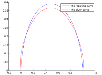
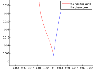
(a)                                             (b)

Figure 1: (a) The rational Bézier curve of degree 4 and the resulting $C^{(1,1)}$ approximation curve of degree 6 as $\rho(t)=\omega(t)$, (b) The photomicrograph of (a) at near zero.

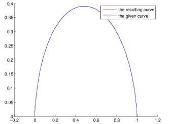
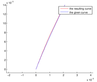
(a)                                             (b)

Figure 2: (a) The rational Bézier curve of degree 4 and the resulting $C^{(1,1)}$ approximation curve of degree 18 as $\rho(t)=\omega(t)$, (b) The photomicrograph of (a) at near zero.

Example 4. (Also Example 1 in [8]). The given curve is a rational Bézier curve of degree $8$ with the control points $(0,0)$, $(0,2)$, $(2,10)$, $(4,6)$, $(6,6)$,$(11,16)$, $(8,1)$, $(9,1)$, $(10,0)$ and the associated weights $1$, $2$, $3$, $9$, $12$, $20$, $30$, $4$, $1$. We find a 5th-degree Bézier curve with different continuity to approximate the given curve, see Table 4. Here, the Hausdorff distance between curves $\textit{{P}}(t)$ and $\textit{{Q}}(t)$ is used. As shown in Table 4. our method is better than Hu’s method for $C^{(1,1)}$-continuity when $\rho(t)=\omega^{2}(t)$.

Table 4: Errors approximation to the rational Bézier curve of degree 8

$C^{(\alpha,\beta)}-\textmd{continuity}$	Hausdorff distance errors
	Hu’s method	$\rho=\omega(t)$	$\rho=\omega^{2}(t)$
$C^{(0,0)}$	0.245371($\lambda$=1.046971)	0.376676194034764	0.487647609642435
$C^{(1,1)}$	0.560612 ($\lambda$=0.713693)	0.576850674814240	0.519236375672234

5 Conclusion

In this paper, we have proposed an algorithm for approximating rational Bézier curves by weighted least-squares. From examples, we can find that approximation methods for $\rho(t)=\omega(t)$ and $\rho(t)=\omega^{2}(t)$ have their advantages and disadvantages respectively. To obtain convex-reserving approximation and reduce the approximation error, higher degree Bézier curve is used in this paper. These two problems are still our future works. Especially, orthogonal polynomials are applied to solve problems .

Acknowledgments. The work is supported by the Natural Science Basic Research Plan in Shaanxi Province of China (No.2013JM1004),the Fundamental Research Funds for the Central Universities (No.GK201102025), the National Natural Science Foundation of China (No.11101253) and the Starting Research Fund from the Shaanxi Normal University (No.999501).

References

• [1] T. W. Sederberg, M. Kakimoto, Approximating rational curves using polynomial curves, in: G. Farin(Ed.), NURBS for curve and surface Design, SIAM, Philadelphia,1991,pp.149-158.
• [2] G. J. Wang, T. W. Sederberg, F. Chen, On the convergence of polynomial of rational functions, Journal Approximation Theory 89 (1997) 267-288.
• [3] G.J. Wang, C. L. Tai, On the convergence of hybrid polynomial approximation to higher derivatives of rational curves, Journal of Computational and Applied Mathematics 214 (2008) 163-174.
• [4] M. S. Folat, High order approximation of rational curves by polynomial curves, Copmuter Aided Geometry Design 23 (2006) 621-628.
• [5] B.G.Lee, Y.B. Park, Approximate Conversion of Rational Bézier Curves,The journal of the Korean Society for Industrial and Applied Mathematics 1 (1998) 88-93.
• [6] Y. Huang,H. Su, H. Lin, A simple method for approximating rational curve using bézier curves, Computer Aided Geometry Design 25 (2008) 697-699.
• [7] L. Z. Lu, Sample-based polynomial approximation of ratinal Bézier curves, Journal of Computational and Applied mathmatics 235 (2011) 1557-1563.
• [8] Q. Q. Hu, H. X. Xu, Constrained polynomial approximation of rational Bézier curves using reparameterization, Journal of Computational and Applied mathmatics 249(2013) 133-143.
• [9] E. Isaacson , Herbert B. Keller, Analysis of Numerical Methods. Dover Publications Inc., 1994.
• [10] G. Farin, Curves and Surfaces for Computer Aided Geomteric Design, Morgan-Kaufmann, San Francisco, 2002.
• [11] G.A. Watson, Approximation Theory and Numerical Methods, John Wiley & Sons, 1980.