Equilibration times in clean and noisy systems

Abstract

We study the equilibration dynamics of closed finite quantum systems and address the question of the time needed for the system to equilibrate. In particular we focus on the scaling of the equilibration time $T_{\mathrm{eq}}$ with the system size $L$. For clean systems we give general arguments predicting $T_{\mathrm{eq}}=O\left(L^{0}\right)$ for clustering initial states, while for small quenches around a critical point we find $T_{\mathrm{eq}}=O\left(L^{\zeta}\right)$ where $\zeta$ is the dynamical critical exponent. We then analyze noisy systems where exponentially large time scales are known to exist. Specifically we consider the tight-binding model with diagonal impurities and give numerical evidence that in this case $T_{\mathrm{eq}}\sim Be^{CL^{\psi}}$ where $B,C,\,\psi$ are observable dependent constants. Finally, we consider another noisy system whose evolution dynamics is randomly sampled from a circular unitary ensemble. Here, we are able to prove analytically that $T_{\mathrm{eq}}=O\left(1\right)$, thus showing that noise alone is not sufficient for slow equilibration dynamics.

I Introduction

Consider a quantum system initialized in a given state and then allowed to evolve undisturbed under the action of a time independent Hamiltonian. Experimentally accessible quantities are expectation values of physical observables $A$ at a given time $\langle A(t)\rangle$. The timescale at which such an expectation value relaxes to equilibrium identifies the equilibration time of the particular dynamics. In infinite systems, equilibration times are typically extracted from the exponential decay of observables or correlation functions towards their equilibrium values. For finite systems, or more generally for systems with discrete energy spectrum, the dynamics is quasi-periodic and such exponential decay cannot occur, thus necessitating a different definition of equilibration time. In these cases a meaningful definition of equilibration time is the first time instant for which the value of an observable equals its equilibrium value, i.e. given an observable $A$ and its equilibrium value $\bar{A}$, $T_{\mathrm{eq}}$ is the smallest $t$ for which $A(t)=\bar{A}$ brandino_quench_2012 .

In this paper we study the behavior of equilibration times according to this definition for various physical systems. In particular we are interested in the scaling behavior of the equilibration time as a function of the linear size of the system .

We first consider equilibration times in clean systems. Using the Loschmidt echo as a particular observable, we are able to give general estimates for the scaling of the $T_{\mathrm{eq}}$ as a function of length. Given a local Hamiltonian $H=\sum_{i}h_{i}$ and a sufficiently clustering initial state $|\psi_{0}\rangle$, i.e. $g_{i,j}=\langle h_{i}h_{j}\rangle-\langle h_{i}\rangle\langle h_{j}\rangle$ decays sufficiently fast as a function of $i-j$ at large separations, we find that $T_{\mathrm{eq}}=O(L^{0})$, i.e. the equilibration time is independent of the system size. This scaling becomes $T_{\mathrm{eq}}=O(L^{\zeta})$ where $\zeta$ is the dynamical critical exponent in case both the initial state and the evolution Hamiltonian are close to a critical point. These general findings are checked explicitly for the Ising chain in a transverse field. However, one should be cautious that these arguments may need modifications for other observables e.g. such as those undergoing spontaneous symmetry breaking.

We then turn our attention to systems with random impurities. According to intuition based on classical models, one expects, in general, a slower transient approach to equilibrium in noisy systems compared to clean systems. Indeed, it is known that exponentially large time-scales are present in glassy systems mcmillan_scaling_1984 . To check and further understand this conjecture, we compute numerically the equilibration time for the tight-binding model with diagonal impurities, sometimes called Anderson model anderson_absence_1958 . A similar model (albeit with pseudo-random diagonal elements) has recently been studied in gramsch_quenches_2012 , where it was found that observables relax following a power-law behavior. Such power-law equilibration pattern (observed also in khatami_quantum_2012 for another noisy system) is itself a signature of slow equilibration. However, according to our definition, equilibration times also depend on the long-time equilibrium value. Our findings confirm a very slow equilibration dynamics characterized by equilibration times diverging exponentially with the system size.

Disorder alone might not be sufficient to guarantee the presence of exponentially large relaxation timescales. To illustrate this point, we analyze a second noisy system. In this case the evolution operator is related to a unitary matrix sampled from the circular unitary ensemble (CUE). This model is similar to the ones previously considered in brandao_convergence_2011 ; cramer_thermalization_2012 , where, according to a different definition, equilibration times decreasing algebraically with the size were predicted cramer_thermalization_2012 . Using our definition we prove analytically that, for the Loschmidt echo, $T_{\mathrm{eq}}=O(1)$.

The paper is organized as follows. In Section II, we describe a clean system and the observables and the quench considered to study the nature of equilibration. Our numerical and analytical results for equilibration timescales and the scaling of these timescales with system length are outlined for the cases of the tight-binding model in Section III and the CUE based evolution in Section IV, respectively. We present our conclusions in Section V.

II Equilibration in clean systems

Before considering noisy systems, let us recall some elementary yet important facts regarding unitary equilibration in clean systems. The system is initialized in some state $\rho_{0}$ which evolves unitarily via $\rho\left(t\right)=e^{-itH}\rho_{0}e^{itH}$. First note that, because of the unitary nature of the evolution, $\rho\left(t\right)$ does not converge in the strong sense as $t\to\infty$. This is true irrespective of the Hilbert space dimension, i.e. also in the thermodynamic limit. One can then consider the possibility of a weaker convergence by looking at “matrix elements” $\mathcal{A}\left(t\right)=\mathrm{tr}\left[A\rho\left(t\right)\right]$ where $A$ is an observable. In the thermodynamic limit the spectrum becomes continuous and one can have limit $\mathcal{A}\left(\infty\right)=\lim_{t\to\infty}\mathcal{A}\left(t\right)$ for some observables $A$ (or appropriately rescaled observables) essentially as a consequence of Riemann-Lebesgue lemma (see e.g. campos_venuti_unitary_2010 and also ziraldo_relaxation_2012 for a recent discussion). For finite systems however, $\mathcal{A}\left(t\right)$ is a trigonometric polynomial and hence, once again, does not admit an infinite time limit. For the same reason though, the time average $\overline{\mathcal{A}}:=\lim_{T\to\infty}\int_{0}^{T}\mathcal{A}\left(t\right)dt$ exists and is finite. Such a time average coincides with the infinite time limit when the latter exists, i.e. $\overline{\mathcal{A}}=\mathcal{A}\left(\infty\right)$. So the time average can be seen as a mathematical trick, reminiscent of Cesaro summation, to obtain the infinite time limit when the function oscillates. Alternatively the time average can mimic the actual measurement process. In this case $T$ is the “observation time” which one may argue to be very large compared to the time scales of the unitary dynamics (see e.g. huang_statistical_1963 ). Clearly one may want to investigate the effect of a finite $T$, here for simplicity we will always take $T\to\infty$.

Because of the above considerations, the standard definition of equilibration time, extracted from the exponential decay of some time dependent observable or correlation function, does not make sense for finite systems, because the dynamics is almost periodic and no exponential decay is possible. Instead, in finite systems, expectation values $\mathcal{A}\left(t\right)$ start from a value $\mathcal{A}\left(0\right)$ which retains memory of the initial state $\rho_{0}$, and then, after an equilibration time, approach an average value $\overline{\mathcal{A}}$ and start fluctuating around it with fluctuations $\delta\mathcal{A}=\sqrt{\overline{\mathcal{A}^{2}}-\overline{\mathcal{A}}^{2}}$ due to the finite dimensionality of the system. Clearly the precise concept of equilibration time is to some extent arbitrary, and different definitions are possible. Ours is the following: $T_{\mathrm{eq}}$ is the first time for which $\mathcal{A}\left(t\right)$ equals the average $\overline{\mathcal{A}}$, i.e. is the first solution of $\mathcal{A}\left(T_{\mathrm{eq}}\right)=\overline{\mathcal{A}}$ (see, for example, fig. 1). This definition is both simple to implement and physically clear.

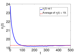
Figure 1: Relaxation of $\mathsf{n}_{\ell}\left(t\right)=\mathsf{E}\left[N_{\ell}\left(t\right)/L\right]$ with time for lengths $L=96$, at filling $\nu=N/L=0.25$ and $\alpha=\ell/L=0.5$. The random distribution has variance $\sigma=0.6$ ($W=0.6\sqrt{3}\approx 1.03$). The ensemble average is computed using 2000 realizations at each time.

Some comments are in order: i) Clearly the precise numerical value of $T_{\mathrm{eq}}$ is irrelevant, whereas the important information is contained in the scaling dependence of $T_{\mathrm{eq}}$ on the system size, $T_{\mathrm{eq}}\left(L\right)$. ii) In principle $\mathcal{A}\left(t\right)$ could intersect $\overline{\mathcal{A}}$ at a first time $T_{1}$, deviate considerably from the average and intersect $\overline{\mathcal{A}}$ again at $T_{2}$, and possibly have multiple intersections up to $T_{n}$ before fluctuations of order $\delta\mathcal{A}$ start to set in. In this situation it seems that the equilibration process cannot be captured by a single $T_{\mathrm{eq}}$ but rather consists of many time scales. In all the situations encountered in our analysis, however, we found that equilibration could always be captured by a single time-scale. iii) The above definition depends on the specific observable $A$ and different observables may have, in principle, different equilibration times. However, we expect that for large classes of observables the scaling dependence with $L$ will be the same. iv) Based on the experience with infinite systems, where observables decay towards their equilibrium value, one could define $T_{\mathrm{eq}}$ as that time for which $\mathcal{A}\left(t\right)$ is off by a small amount from its average value $\overline{\mathcal{A}}$. This is, after all, the definition we use in the thermodynamic limit when the approach to equilibrium is exponential. A definition of this sort has been used for instance in cramer_thermalization_2012 . In this way, however, $T_{\mathrm{eq}}$ depends in principle on the way we define small.

To test the equilibration time we consider a particular observable, the Loschmidt echo (LE) which we define as

$$\mathcal{L}\left(t\right)=\left|\langle\psi_{0}|e^{-itH}|\psi_{0}\rangle\right|^{2}\,,$$ (1)

where $|\psi_{0}\rangle$ is the state in which we initialize the system and $H$ the evolution Hamiltonian. The Loschmidt echo has been first introduced in the context of quantum chaos (see e.g. gorin_dynamics_2006 ), and is generally given a more general form in that context. Equation (1) can be seen as the time evolved expectation value of the observable $|\psi_{0}\rangle\langle\psi_{0}|$, and is also known as survival probability. Here we consider the LE because it is amenable of a cumulant expansion which correctly approximates $\mathcal{L}\left(t\right)$ for sufficiently large times of the order of $T_{\mathrm{eq}}$. This conclusion is based on numerical experiments on the Ising model in transverse field campos_venuti_unitary_2010 . A hand waving argument is the following: since $\mathcal{L}$ is morally a product of $L^{d}$ terms (see below) it should be clear that Taylor expansion of $\ln\mathcal{L}$ works better than the Taylor expansion of $\mathcal{L}$ itself. The cumulant expansion of Eq. (1) reads

$$\mathcal{L}\left(t\right)=\exp\left[2\sum_{n=1}^{\infty}\frac{\left(-t^{2}\right)^{n}}{\left(2n\right)!}\langle H^{2n}\rangle_{c}\right]\,,$$ (2)

where $\langle\cdot\rangle_{c}$ stands for connected average with respect to $|\psi_{0}\rangle$. Truncating Eq. (2) up to the first order we obtain $\mathcal{L}\left(t\right)\simeq\exp\left[-t^{2}\left(\Delta H^{2}\right)\right]$ ($\Delta H^{2}=\langle H^{2}\rangle-\langle H\rangle^{2}$). Equating the short time expansion to the average value $\overline{\mathcal{L}}$ we get the following expression for the equilibration time:

$$T_{\mathrm{eq}}=\sqrt{\frac{-\ln\overline{\mathcal{L}}}{\Delta H^{2}}}\,.$$ (3)

As we will see, the above estimate for $T_{\mathrm{eq}}$ works well for the Loschmidt echo Eq. (1). Some comments are in order at this point. First of all, the equilibration time in Eq. (3) is inversely proportional to the square root of an energy fluctuation. This is not simply the inverse of an energy gap as one might guess naïvely. Secondly, we would like to compare Eq. (3), with another estimate of equilibration time which appeared recently in a single body setting yurovsky_dynamics_2011 . The estimate of yurovsky_dynamics_2011 reads $T_{\mathrm{eq}}\sim 1/\langle\Delta E_{\mathrm{min}}\rangle_{\mathrm{ave}}$, where $\Delta E_{\mathrm{min}}$ is the minimum energy gap averaged over an energy shell around the initial energy $\langle H\rangle$ . So, apart from the order of averages, the equilibration time in yurovsky_dynamics_2011 is inversely proportional to a standard deviation of an energy fluctuation as much as in Eq. (3). The definitions differ in the numerator which takes into account the many-body nature of the problem. Thirdly, the estimate Eq. (3) is valid only for the equilibration time of the Loschmidt echo, and in principle, different observables might equilibrate with different time scales.

We will now provide arguments to estimate Eq. (3) which first appeared in campos_venuti_unitary_2010 . For a local Hamiltonian $H=\sum_{i}h_{i}$ and a sufficiently clustering initial state $|\psi_{0}\rangle$, i.e. $g_{i,j}=\langle h_{i}h_{j}\rangle-\langle h_{i}\rangle\langle h_{j}\rangle$ decays sufficiently fast as a function of $i-j$ at large separations, all the cumulants in Eq. (2) are extensive in the system size, that is in a $d$-dimensional system of linear size $L$, $\langle H^{2n}\rangle_{c}\propto L^{d}$. This means that at leading order in $L$, $\mathcal{L}\left(t\right)\simeq e^{f\left(t\right)L^{d}}$ and so, by Jensen’s inequality $e^{\overline{f}L^{d}}\leq\overline{\mathcal{L}}\leq\exp[L^{d}\max_{t}f\left(t\right)]$, showing that $\overline{\mathcal{L}}$ is exponentially small in the system volume (note that we must have $f\left(t\right)\leq 0$). For this reason it is sometimes useful to consider the logarithm of the LE $\mathcal{F}\left(t\right)=\ln\mathcal{L}\left(t\right)$. The equilibration time for $\mathcal{F}$ would then be given by $T_{\mathrm{eq}}^{\mathcal{F}}=\sqrt{-\overline{\ln\mathcal{L}}/\Delta H^{2}}$. Now, since $\overline{\ln\mathcal{L}}\simeq\overline{f\left(t\right)}L^{d}$, we see that the equilibration times for $\mathcal{L}$ and $\mathcal{F}=\ln\mathcal{L}$ are expected to give the same scaling with respect to $L$. From equation (2) we get then $T_{\mathrm{eq}}=O\left(1\right)$: the equilibration time is independent of the system size. This argument fails when one considers small quenches close to a quantum critical point as in this case the clustering properties of the initial state tends to break down. In this case $|\psi_{0}\rangle$ is the ground state of $H_{0}=H\left(\lambda_{0}\right)$ where the external parameter $\lambda_{0}$ is close to a quantum critical point. One then suddenly changes the parameters by a small amount $\lambda_{0}\to\lambda_{0}+\delta\lambda$ and the system is let evolve undisturbed with Hamiltonian $H=H\left(\lambda_{0}+\delta\lambda\right)$. In the very small quench regime, roughly $\delta\lambda\ll\min\{L^{-1/\nu},L^{-2/d}\}$ where $\nu$ is the correlation length exponent, perturbation theory is applicable (see below) and the average LE reduces to $\overline{\mathcal{L}}\approx\left|\langle\psi_{0}|0\rangle\right|^{4}$, where $|0\rangle$ is the ground state of $H$ rossini_decoherence_2007 . The scaling properties of the fidelity $\left|\langle\psi_{0}|0\rangle\right|$ close to a quantum critical point have been studied in campos_venuti_quantum_2007 where it was shown that $\left|\langle\psi_{0}|0\rangle\right|\approx 1-\mathrm{const.}\times\delta\lambda^{2}L^{2\left(d+\zeta-\Delta\right)}$, where $\zeta$ is the dynamical critical exponent, and $\Delta$ the scaling dimension of the operator driving the transition. Using similar scaling arguments one can show that the variance scales as $\langle H^{2}\rangle_{c}\approx L^{2\left(d-\Delta\right)}$ campos_venuti_unitary_2010 . These results are valid in the perturbative regime where $\left|\langle\psi_{0}|0\rangle\right|$ is not too far from 1, i.e. $\delta\lambda\ll\min\{L^{-1/\nu},L^{-2/d}\}$ where $\nu=\left(d+\zeta-\Delta\right)^{-1}$ campos_venuti_quantum_2007 . From equation (2) we now get $T_{\mathrm{eq}}=O\left(L^{\zeta}\right)$, i.e. the equilibration time diverges for large systems. Such a divergence is reminiscent of the critical slowing down observed in quantum Monte Carlo algorithms.

II.1 Quantum Ising model

As a concrete example we now consider equilibration times and in particular the prediction Eq. (3) for the quantum Ising model undergoing a sudden field quench. The Hamiltonian is

$$H=-\sum_{j=1}^{L}\left[\sigma_{j}^{x}\sigma_{j+1}^{x}+h\sigma_{j}^{z}\right],$$ (4)

and periodic boundary conditions are used. The system is initialized in the ground state of Eq. (4) with parameter $h^{\left(1\right)}$. At time $t=0$, the parameter is suddenly changed to $h^{\left(2\right)}$ and the state is let evolve unitarily with Hamiltonian $H\left(h_{2}\right)$. The model in Eq. (4) has critical points in the Ising universality class at $h=\pm 1$ with $d=\nu=\zeta=1$, separating an ordered phase $\left|h\right|<1$ from a disordered paramagnetic region $\left|h\right|>1$. For $\left|h\right|<1$ the order parameter $\langle\sigma_{i}^{x}\rangle$ becomes non-zero, thus breaking the $\mathbb{Z}_{2}$ symmetry ($\sigma_{i}^{x}\to-\sigma_{i}^{x}$) of the Hamiltonian.

According to Eq. (3) and the discussion of the previous section we expect the following behavior for the equilibration time as a function of the quench parameters $h_{2},\,\delta h=h_{2}-h_{1}$ and system size $L$:

$$T_{\mathrm{eq}}\propto\begin{cases}L&\mathrm{for}\,\,h_{2}=h_{c},\,\,\mathrm{and}\,\,\delta h\ll L^{-1}\\ \mathrm{const.}&\mathrm{otherwise}\end{cases}$$ (5)

As a first test we check whether Eq. (5) is satisfied for the Loschmidt echo itself. The LE for a sudden quench has been computed in quan_decay_2006 (superscripts refer to to different values of the coupling constants $h^{\left(i\right)}$)

$$\mathcal{L}\left(t\right)=\prod_{k>0}\left[1-\sin^{2}\left(\delta\vartheta_{k}\right)\sin^{2}\left(\Lambda_{k}^{\left(2\right)}t/2\right)\right]$$

where $\Lambda_{k}=2\sqrt{1+h^{2}+2h\cos(k)}$ is the single particle dispersion, $\delta\vartheta_{k}=\vartheta_{k}^{\left(2\right)}-\vartheta_{k}^{\left(1\right)}$ and $\vartheta_{k}^{\left(i\right)}$ are the Bogoliubov angles at parameters $h^{\left(i\right)}$, and the quasimomenta are quantized according to $k=\pi\left(2n+1\right)/L,\,n=0,1,\ldots L/2-1$ (see campos_venuti_unitary_2010 for further details). In Fig. 2 we plot the equilibration time $T_{\mathrm{eq}}^{\mathcal{L}}$ of the Loschmidt echo versus size for different quench parameters computed exactly by solving numerically for the first solution of $\mathcal{L}\left(t\right)=\overline{\mathcal{L}}$. Indeed Eq. (5) is satisfied to a high accuracy. Moreover the transition between the two behaviors of Eq. (5) appears to be very sharp. From the numerical analysis the following behavior for $T_{\mathrm{eq}}^{\mathcal{L}}$ emerges valid outside the crossover region $\delta h\approx cL^{-1}$

$$T_{\mathrm{eq}}^{\mathcal{L}}=\begin{cases}\frac{L}{4}&\mathrm{for}\,\,h_{2}=h_{c},\,\,\mathrm{and}\,\,\delta h\ll cL^{-1}\\ \frac{c}{4\delta h}&\mathrm{otherwise}\end{cases},$$

where the constant $c$ in principle depends on $h_{1},\,h_{2}$, but for small quenches close to the critical point tends to $c\simeq 6.1$. The typical behavior in the crossover region $\delta h\simeq cL^{-1}$ is depicted in Fig. 3.

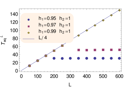
Figure 2: Equilibration times $T_{\mathrm{eq}}^{\mathcal{L}}$ for the Loschmidt echo as a function of the system size $L$ for different quench parameters $h_{1,2}$. $T_{\mathrm{eq}}^{\mathcal{L}}$ is computed by solving numerically for the first solution of $\mathcal{L}\left(t\right)=\overline{\mathcal{L}}$.

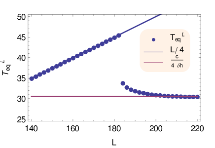
Figure 3: Equilibration times $T_{\mathrm{eq}}^{\mathcal{L}}$ for the Loschmidt echo close to the crossover region $\delta h\simeq cL^{-1}$.

It is natural to ask whether the predictions of Eq. (5) are satisfied for observables other than the Loschmidt echo. To this end, we consider the transverse magnetization $m^{z}\left(t\right)=\langle\sigma_{i}^{z}\left(t\right)\rangle$ which can be computed as barouch_statistical_1970 ; campos_venuti_unitary_2010

$$m^{z}\left(t\right)=\frac{1}{L}\sum_{k}\cos\left(\vartheta_{k}^{\left(2\right)}\right)\cos\left(\delta\vartheta_{k}\right)\\ +\sin\left(\vartheta_{k}^{\left(2\right)}\right)\sin\left(\delta\vartheta_{k}\right)\cos\left(t\Lambda_{k}^{\left(2\right)}\right)$$ (6)

From eq. (6) we extract the equilibration time from the solution of $m^{z}\left(t\right)=\overline{m^{z}}=L^{-1}\sum_{k}\cos\left(\vartheta_{k}^{\left(2\right)}\right)\cos\left(\delta\vartheta_{k}\right)$. The numerical results, shown in Fig. 4, confirm that Eq. (3) is applicable to the transfer magnetization too. The numerical results can be summarized as

$$T_{\mathrm{eq}}^{m^{z}}=\begin{cases}\frac{L}{4}&\mathrm{for}\,\,h_{2}=h_{c},\,\,\mathrm{and}\,\,\delta h\ll c^{\prime}L^{-1}\\ \frac{c^{\prime}}{4\delta h}&\mathrm{otherwise}\end{cases}$$

with constant given now by $c^{\prime}\simeq 15$ for small quenches close to criticality.

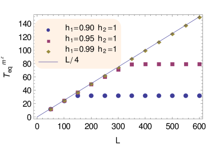
Figure 4: Equilibration times $T_{\mathrm{eq}}^{m^{z}}$ for the transverse magnetization $m^{z}\left(t\right)=\langle\sigma_{1}^{z}(t)\rangle$ as a function of the size $L$ for different quench parameters $h_{1,2}$. $T_{\mathrm{eq}}^{m^{z}}$ is computed exactly solving for the first solution of $m^{z}\left(t\right)=\overline{m^{z}}$.

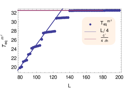
Figure 5: Equilibration times $T_{\mathrm{eq}}^{m^{z}}$ for the transverse magnetization close to the crossover region $\delta h\simeq c^{\prime}L^{-1}$. For this values of parameters $c^{\prime}\simeq 13$.

Finally, let us comment on the approach to equilibrium of the order parameter $m^{x}\left(t\right)=\langle\sigma_{i}^{x}\left(t\right)\rangle$. We recall that, since a non-zero $m^{x}$ breaks the symmetry of the Hamiltonian, $m^{x}$ must be computed as the clustering part of an equal time correlation function: $\langle\sigma_{i}^{x}\left(t\right)\sigma_{j}^{x}\left(t\right)\rangle\stackrel{{\scriptstyle\left|i-j\right|\to\infty}}{{\longrightarrow}}\left[m^{x}\left(t\right)\right]^{2}$. As usual in symmetry broken phases this requires the thermodynamic limit to be taken first, but a finite size approximation for systems with periodic boundary conditions can be obtained by considering the correlation at half chain $\left[m_{L}^{x}\left(t\right)\right]^{2}:=\langle\sigma_{i}^{x}\left(t\right)\sigma_{i+L/2}^{x}\left(t\right)\rangle$.

We do not expect formula (3) to reproduce the equilibration time correctly for the order parameter, as it does not distinguish whether we are in the ordered phase or not.

The behavior of $m^{x}\left(t\right)$ has recently been obtained analytically in the thermodynamic limit in the quench setting calabrese_quantum_2012 . The results of calabrese_quantum_2012 for $m^{x}\left(t\right)$ can be summarized as follows. First of all $m^{x}\left(t\right)=0$ identically for quenches starting in the disordered phase $(\left|h_{1}\right|>1$) as the symmetry remains unbroken. For quenches starting in the ordered phase $(\left|h_{1}\right|<1)$ one has a different behavior depending whether one ends up in the ordered or disordered phase. More specifically

$$m^{x}\left(t\right)=\begin{cases}Ae^{-t/\tau}&\left|h_{2}\right|<1\\ A^{\prime}e^{-t/\tau}\sqrt{1+\cos\left(\Lambda_{k_{0}}t+\alpha\right)+\ldots}&\left|h_{2}\right|>1\end{cases}$$

The constants $A,\,A^{\prime},\,\tau,\,k_{0},\,\alpha$ all depends on $h_{1},\,h_{2}$ and are given explicitly in calabrese_quantum_2012 . For quenches starting end ending in the ordered region, the equation $m^{x}\left(t\right)=\overline{m^{x}}=m^{x}\left(\infty\right)=0$ has no real solution. Correspondingly at finite size, $T_{\mathrm{eq}}^{m^{x}}$ must be an increasing function of $L$ and the simplest guess is $T_{\mathrm{eq}}^{m^{x}}\propto L^{\zeta}=L$. Instead for quenches ending in the disordered region, we see that $m^{x}\left(t\right)=0$ has a finite solution even in the thermodynamic limit, and so we expect in this case $T_{\mathrm{eq}}^{m^{x}}=O\left(L^{0}\right)$.

III The Anderson model

We now turn to random systems. The model we consider is the tight-binding model with random diagonal disorder, sometimes referred to as the Anderson model anderson_absence_1958 :

$$H=\sum_{j=1}^{L}\left[t\left(c_{j}^{\dagger}c_{j+1}+c_{j+1}^{\dagger}c_{j}\right)-\mu_{i}c_{i}^{\dagger}c_{i}\right].$$ (7)

The diagonal elements $\mu_{i}$ are identically distributed independent random variables. In all of our simulations we will use a uniform, flat distribution in the interval $\left[-W,W\right]$. Through the Jordan-Wigner mapping, Hamiltonian Eq. (7) equivalently describes an $XX$ chain of $L$ spins in a random magnetic field. The Hamiltonian Eq. (7) can be written in compact notation as $H=c^{\dagger}M_{\mu}c$ , where $c=\left(c_{1},\ldots,c_{L}\right)^{T}$, $M_{\mu}$ is the one particle Hamiltonian and the subscript $\mu$ refers to the random variables $\mu_{i}$. In the infinite volume limit, the spectrum of $M_{\mu}$ is given, with probability one, by $\sigma\left(\nabla^{2}\right)+\mathrm{supp}\left(-\mu_{i}\right)=\left[-2t,2t\right]+\mathrm{supp}\left(-\mu_{i}\right)$ where $\nabla^{2}$ is the discrete Laplacian in 1D, $\left(\nabla^{2}\right)_{i,j}=\delta_{i,j+1}+\delta_{i,j-1}$, and $\mathrm{supp}$ is the support. In case of a uniform distribution we have $\sigma\left(M_{\mu}\right)=\left[-2t-W,2t+W\right]$. Moreover, for any finite amount of randomness, the spectrum is almost surely pure point, i.e. consists only of eigenvalues, and the eigenfunctions are exponentially localized (see e.g. kunz_sur_1980 ; frohlich_constructive_1985 ). Such a situation is referred to as a localized phase. Since in the absence of disorder the model Eq. (7) is a band conductor, in one spatial dimension there is a metal-insulator transition for any however small amount of disorder $W>0$.

To study the equilibration properties of the Anderson model, we proceed as follows. We initialize the system in a state $\rho_{0}$, evolve it unitarily with one instance of Hamiltonian Eq. (7) into $\rho\left(t\right)$, and consider the expectation value of some observable $A$: $\mathcal{A}\left(t\right)=\mathrm{tr}\left(A\rho\left(t\right)\right)$. For very large systems one expects that concentration results will apply and that the single instance $\mathcal{A}\left(t\right)$ will be, with very large probability, close to its ensemble average $\mathsf{A}\left(t\right):=\mathsf{E}\left[\mathcal{A}\left(t\right)\right]$ where we denoted with $\mathsf{E}\left[\cdot\right]$ the average over the random potentials $\mu_{i}$. When this happens, or more precisely when the relative variance $\Delta^{2}\mathsf{A}/\mathsf{A}^{2}\to 0$ as the system size increases, one says that $\mathcal{A}$ is self-averaging. We will not be concerned with this issue here, we just notice that $\mathsf{A}\left(t\right)$ generally gives the result of a hypothetical measurement of $A$ within the confidence interval. The equilibration time is then obtained by solving for the first solution of $\mathsf{A}(T_{\mathrm{eq}})=\overline{\mathsf{A}}$.

To be concrete we will consider a Gaussian initial state $\rho_{0}$ with $N$ particles uniquely specified by the covariance matrix $R_{i,j}=\mathrm{tr}(c_{i}^{\dagger}c_{j}\rho_{0})$. Since Eq. (7) conserves particle number, the evolution is constrained to the sector with $N$ particles. As observables, we choose a general quadratic operator given by $A=\sum_{i,j}a_{i,j}c_{i}^{\dagger}c_{j}$. In this case the expectation value $\mathcal{A}\left(t\right)$ can be completely characterized in terms of one-particle matrices campos_venuti_gaussian_2012 :

$$\mathcal{A}\left(t\right)=\mathrm{tr}\left[A\rho\left(t\right)\right]=\mathrm{tr}\left(ae^{-itM_{\mu}}R^{T}e^{itM_{\mu}}\right)\,.$$ (8)

To be specific we will study two particular quadratic observables: $N_{\ell}:=\sum_{j=1}^{\ell}c_{i}^{\dagger}c_{i}$ which counts how many particles are present in the first $\ell$ sites (say from left). In this case the thermodynamic limit is given by fixing the particle density $\nu=N/L$ together with the “observable” density $\alpha=\ell/L$ and let $L\to\infty$.

As previously argued, a useful quantity to consider is the LE. In this free Fermionic setting it can be written as klich_full_2002 ; peschel_calculation_2003

$$\mathcal{L}\left(t\right)=\left|\det\left(1-R^{T}+R^{T}e^{-itM_{\mu}}\right)\right|^{2}\,.$$

Because of the random nature of the problem we do not expect the initial locations of the $N$ particles to matter particularly. Hence we will consider an initial state where all the $N$ particles are pushed to the left, i.e. $R_{i,i}=1$ for $i=1,2,\ldots,N$ and all other entries zero. We have checked that initializing the particles at other sites does not change our results. In any case for pure initial states, $R^{T}$ is a (orthogonal) projector $\left(R^{T}\right)^{2}=R^{T}$, meaning its eigenvalues are either 1 or 0. Therefore, in some basis, $R^{T}$ always has the aforementioned form, i.e. there exists a unitary matrix $X$ such that $X^{\dagger}R^{T}X=R_{N}^{T}=\mathrm{diag}\left(1,1,\ldots,1,0,\ldots,0\right)$ with $N$ entries $1$ and $\left(L-N\right)$ zeros. The Loschmidt echo then becomes $\mathcal{L}\left(t\right)=\left|\det\left(1-R_{N}^{T}+R_{N}^{T}X^{\dagger}e^{-itM}X\right)\right|^{2}$. Our choice of initial state corresponds to having $X=\leavevmode{\rm 1\mkern-4.8muI}$. Thanks to the simple form of $R_{N}^{T}$, one can evaluate the determinant using Laplace’s formula and reduce it to a determinant of an $N\times N$ matrix, i.e.

$$\mathcal{L}\left(t\right)=\left|\det\Gamma_{N}\left[X^{\dagger}e^{-itM}X\right]\right|^{2}$$

where the operator $\Gamma_{N}\left[Y\right]$ truncates the last $L-N$ rows and columns of $Y$. Since clearly $\left\|\Gamma_{N}\left[U\right]\xi\right\|\leq\left\|\xi\right\|$ for any unitary matrix $U$ and $L$-dimensional complex vector $\xi$, the eigenvalues of $\Gamma_{N}\left[X^{\dagger}e^{-itM}X\right]$, $z_{i}\left(t\right)$ have modulus smaller than one. The LE can than be written as

$$\mathcal{L}\left(t\right)=e^{\mathcal{F}\left(t\right)}=e^{\nu Lf\left(t\right)}$$

having defined $f\left(t\right)=\left(1/N\right)\sum_{i=1}^{N}\ln\left|z_{i}\left(t\right)\right|^{2}$. Provided $f\left(t\right)$ has a limit as $L\to\infty$, this shows that $\mathcal{L}\left(t\right)$ is exponentially small in the system size. Accordingly, since $\mathcal{F}\left(t\right):=\ln\mathcal{L}\left(t\right)$ is extensive, we expect it to be self-averaging and convenient to study. We also consider the averaged Loschimdt echo $\mathsf{L}\left(t\right)=\mathsf{E}\left[\mathcal{L}\left(t\right)\right]$ and the ensemble average of the logarithm of the Loschimidt echo (LLE) $\mathsf{F}\left(t\right)=\mathsf{E}\left[\mathcal{F}\left(t\right)\right]$. Note that by Jensen’s inequality $\mathsf{L}\left(t\right)\geq e^{\mathsf{F}\left(t\right)}$.

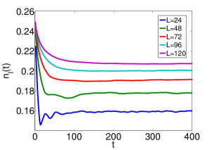
Figure 6: Relaxation of $\mathsf{n}_{\ell}\left(t\right)=\mathsf{E}\left[N_{\ell}\left(t\right)/L\right]$ with time for lengths $L=16,\,40,\,64,\,112$, at filling $\nu=N/L=0.25$ and $\alpha=\ell/L=0.5$. The random distribution has variance $\sigma=0.6$ ($W=0.6\sqrt{3}\approx 1.03$). The ensemble average is computed using 1000 realizations at each time.

In Fig. 6 we show the results of our numerical simulations for the –ensemble averaged– observable $\mathsf{n}_{\ell}\left(t\right)=\mathsf{E}\left[N_{\ell}\left(t\right)/L\right]$. When computing the equilibration time for observable $A$ by looking for the first solution of $\mathsf{A}(T_{\mathrm{eq}})=\overline{\mathsf{A}}$, the computationally most demanding part is the calculation of $\overline{\mathsf{A}}$, especially for large system sizes. For quadratic observables, this computation can be simplified considerably. We first note that the time and ensemble averages commute. This is essentially a consequence of Fubini’s theorem and the fact that all our quantities are bounded. The time average of $\mathcal{A}\left(t\right)$ for a particular realization can be computed diagonalizing $M_{\mu}$. With the notation $M_{\mu}=Q^{\dagger}\Lambda Q$, $\Lambda=\mathrm{diag}\left\{\epsilon_{1},\ldots,\epsilon_{L}\right\}$, and $Q$ unitary, one has $\mathcal{A}\left(t\right)=\sum_{n,m}\left(Q^{\dagger}AQ\right)_{n,m}\left(Q^{\dagger}R^{T}Q\right)_{m,n}e^{-it\left(\epsilon_{m}-\epsilon_{n}\right)}$. Now, simply note that, with probability one, the spectrum $\epsilon_{n}$ is non-degenerate. This implies that the time average is given exactly by

$$\overline{\mathcal{A}}=\sum_{n}\left(Q^{\dagger}AQ\right)_{n,n}\left(Q^{\dagger}R^{T}Q\right)_{n,n}$$ (9)

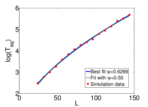
Figure 7: Scaling of equilibration time $T_{\mathrm{eq}}(L)$ vs system size $L$, extracted from $\mathsf{n}_{\ell}\left(t\right)$. $T_{\mathrm{eq}}$ is obtained from this first solution of $\mathsf{E}[n_{\ell}(T_{\mathrm{eq}})]=\overline{\mathsf{E}[n_{\ell}(t)]}$. Parameters are as in Figure 6 . The ensemble averages are obtained summing over 2000 realizations. The equilibration time is found to obey $\log(T_{\mathrm{eq}})=0.021L^{0.6266}+2.53$ with residual norm $0.17$.

The value $\overline{\mathsf{A}}$ is then computed taking the ensemble average of $\overline{\mathcal{A}}$, $\overline{\mathsf{A}}=\mathsf{E}\left[\overline{\mathcal{A}}\right]$, using Eq. (9). In figure 7 we plot the equilibration time obtained for $\mathsf{n}_{\ell}\left(t\right)$ as a function of system size $L$. Our numerical results show that the equilibration time scales exponentially in the system size.

For the case of the LE and the LLE we have not been able to compute the time average exactly. It is known that in case of non-degenerate many body energies, which is safe to assume in presence of randomness, one has $\overline{\mathcal{L}}=\sum_{n}\left|\langle\psi_{0}|\left\{n\right\}\rangle\right|^{4}$ campos_venuti_unitary_2010 (where $|\left\{n\right\}\rangle=|n_{1},\ldots,n_{L}\rangle$’s are the many-body eigenfunctions satisfying $\sum_{j}n_{j}=N$). For our choice of initial state, the amplitudes are given by

$$\langle\psi_{0}|\left\{n\right\}\rangle=\det V_{\left[1,2,\ldots,N\right]}Q^{\dagger}V_{\left\{n\right\}}^{\dagger}$$

where $V_{\left[1,\ldots,N\right]}$ is the $N\times L$ matrix with ones on the diagonal and zero otherwise. $V_{\left\{n\right\}}$ is formed in the same way but the ones on the diagonal are in correspondence of the row $i$ for which $n_{i}=1$. The normalization of the weights is provided by Cauchy-Binet’s formula

$$\sum_{\stackrel{{\scriptstyle\left\{n\right\}}}{{\sum_{i}n_{i}=N}}}\det V_{\left[1,2,\ldots,N\right]}Q^{\dagger}V_{\left\{n\right\}}^{\dagger}\det V_{\left\{n\right\}}TQV\\ =\det V_{\left[1,2,\ldots,N\right]}Q^{\dagger}QV_{\left[1,2,\ldots,N\right]}^{\dagger}=1$$

The time average Loschmidt echo is then given by

$$\overline{\mathcal{L}}=\sum_{\stackrel{{\scriptstyle\left\{n\right\}}}{{\sum_{i}n_{i}=N}}}\left|\det V_{\left[1,2,\ldots,N\right]}Q^{\dagger}V_{\left\{n\right\}}^{\dagger}\right|^{4}$$

The above sum, however, contains an exponential number of terms and is not practical for numerical computations. To evaluate $\overline{\mathsf{L}}$ and $\overline{\mathsf{F}}$, we compute the $\mu$-random average $\mathsf{L}\left(t\right)\simeq N_{\mathrm{samples}}^{-1}\sum_{i=1}^{N_{\mathrm{samples}}}\mathcal{L}_{i}\left(t\right)$ (and similarly for $\mathsf{F}$) using as many as $N_{\mathrm{samples}}=2000$ for $N_{\mathrm{times}}$ random times uniformly distributed between $\left[T_{0},T\right]$. The time average is then obtained via $\overline{\mathsf{L}}\simeq N_{\mathrm{samples}}^{-1}N_{\mathrm{times}}^{-1}\left(T-T_{0}\right)^{-1}\sum_{j=1}^{N_{\mathrm{times}}}\sum_{i=1}^{N_{\mathrm{samples}}}\mathcal{L}_{i}(t_{j})$. We use a positive $T_{0}$ to get rid of the initial transient and obtain more precise estimates with the same computational cost. Typical valued we used are $T\simeq 1000$, $T_{0}\simeq 750$. Larger times of the order of $T\simeq 10000$ with $T_{0}\simeq 1000$ were used for systems of size exceeding $L\sim 128$.

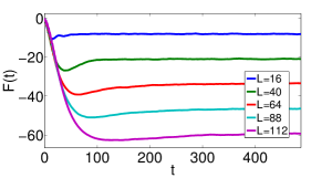
Figure 8: Relaxation of $\mathsf{F}(t)=\mathsf{E}[\log(\mathcal{L}(t))]$. Parameters are as in Figure 6 and an ensemble average was performed over 1000 realizations at each instant in time.

In figure 8 we plot the ensemble averaged LLE time series $\mathsf{F}\left(t\right)$ at different sizes $L$ while in figure 9 we show the equilibration times of the logarithmic Loschmidt echo as a function of $L$ . In this case as well, the numerical results indicate equilibration times diverging exponentially in the system size. Based on the numerical evidence, we conjecture that for more general observables $O$, the equilibration time in the Anderson model might satisfy

$$\ln T_{\mathrm{eq}}^{O}=c_{O}L^{\psi}+d_{O}$$

where $c_{O},\,d_{O},\,\psi$ are constants which depend on the observable $O$.

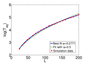
Figure 9: Scaling of the relaxation time $T_{eq}$ such that $\mathsf{F}(T_{eq})=\overline{\mathsf{F}}$ , $T_{eq}=1.39L^{0.2771}-0.847$ with residual norm $0.05$.

IV A CUE model

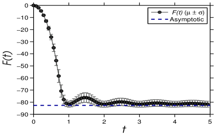
Figure 10: Plot of $\mathsf{F}\left(t\right)$ for $L=120$, at $\nu=1/2$ (half filling). The variance $\delta\mathsf{F}\left(t\right)$ is shown as error bar. Numerical results are obtained averaging over $N_{\mathrm{samples}}=7500$ unitaries distributed according to the Haar measure and obtained with the algorithm outlined in mezzadri_how_2006 .

In this section we consider another random matrix model for which we are able to prove analytically that $T_{\mathrm{eq}}\leq 1$. In this model we fix the evolution operator $U$ at time $t=1$ to be taken from the circular unitary ensemble (CUE). This means that $U$ is an $L\times L$ unitary matrix sampled from the uniform Haar measure over the group $\mathbb{U}\left(L\right)$. At other times the evolution is defined via $U^{t}$. The arbitrariness in the definition of $U^{t}$ for $t\in\mathbb{R}$ is fixed in the following way. Any unitary matrix $U$ from the CUE can be written as $U=V^{\dagger}e^{i\boldsymbol{\phi}}V$ where $V$ is again Haar distributed, $e^{i\boldsymbol{\phi}}:=\mathrm{diag}(e^{i\phi_{1}},e^{i\phi_{2}},\ldots,e^{i\phi_{L}})$ and the phases $\phi_{i}$ are distributed according to $P\left(\boldsymbol{\phi}\right)=C\prod_{i<j}\left|e^{i\phi_{i}}-e^{i\phi_{j}}\right|^{2}$ where $C^{-1}=\left(2\pi\right)^{L}L!$ is the normalization constant and $\phi_{i}\in[0,2\pi)$ (see e.g. mehta_random_2004 ). Our model is described by taking a Hamiltonian $H=\boldsymbol{\phi}:=\mathrm{diag}(\phi_{1},\phi_{2},\ldots,\phi_{L})$ and considering the average over all isospectral Hamiltonians $H^{\prime}=V^{\dagger}HV$ with $V$ Haar distributed. The dynamical evolution is given by $e^{itH^{\prime}}$. Given these considerations this model is equivalent to the ensemble considered in brandao_convergence_2011 ; cramer_thermalization_2012 after averaging all the energies $E_{i}$ with the CUE distribution $P\left(\boldsymbol{\phi}\right)$. Let us now turn to the computation of $\mathsf{F}\left(t\right)=\mathsf{E}_{U}\left[\ln\det\Gamma_{N}\left(e^{itH^{\prime}}\right)\right]$. If $t=n$ is an integer, the evolution operator is given by $e^{itH^{\prime}}=U^{n}$ where $U^{n}$ is unitary and Haar distributed, hence, at integer times we obtain

$$\mathsf{F}\left(n\right)\equiv\mathsf{F}_{0}=\mathsf{E}_{U}\left[\ln\left|\det\Gamma_{N}(U)\right|^{2}\right],$$

independent of $n$. We observed, as it is natural to expect, that the function $\mathsf{F}\left(t\right)$ has a limit as $t\to\infty$ (see Fig. 10). In this case the limit must coincide with the time average and with $\mathsf{F}(n)$ for $n$ integer, i.e. $\mathsf{F}\left(\infty\right)=\mathsf{F}(n)=\overline{\mathsf{F}}$. This shows that the relaxation time in this random systems is bounded by one. In fact in principle one could have $\mathsf{F}\left(t\right)=\overline{\mathsf{F}}$ also for a time $t$ smaller than one, however our numerics indicates that the first occurrence of $\mathsf{F}\left(t\right)=\overline{\mathsf{F}}$ is indeed at $T_{\mathrm{eq}}=1$ (see Fig. 10) independent of the system size. We would like to mention at this point the results of Ref. brandino_quench_2012 where a different sparse random ensemble has been constructed and an equilibration time growing as the system size has been reported. These findings show that random systems can give rise, in general, both to slow and fast equilibration processes and the correct equilibration time-scale can only be obtained through an accurate investigation (although one expects faster equilibration to be associated to less sparse Hamiltonians).

It turns out that the limiting value $\mathsf{F}\left(\infty\right)$ can be obtained exactly. The distribution of eigenvalues of truncated matrices $\Gamma_{N}(U)$ when $U$ is Haar distributed has been computed in zyczkowski_truncations_2000 . The eigenvalues $z_{i}$ of $\Gamma_{N}(U)$ are complex numbers in the unit disk $\left|z_{i}\right|\leq 1$. Calling $r_{i}=\left|z_{i}\right|$, and defining the probability distribution of the moduli $P_{L,N}\left(r\right)\equiv N^{-1}\sum_{i=1}^{N}\mathsf{E}_{U}\left[\delta\left(r-\left|z_{i}\right|\right)\right]$, the CUE average at integers time is then given by

$$\mathsf{F}_{0}=N\int_{0}^{1}P_{L,N}\left(r\right)\ln\left(r^{2}\right)dr.$$ (10)

Zyczkowski and Sommers were able to compute the distribution of the moduli $P_{L,N}(r)$ and obtained, with $x=r^{2}$

$$P\left(r\right)=\frac{2r}{N}\frac{\left(1-x\right)^{L-N-1}}{\left(L-N-1\right)!}\left(\frac{d}{dx}\right)^{L-N}\frac{1-x^{L}}{1-x}.$$

The probability density $P_{\nu}\left(r\right)$ in the thermodynamic limit at fixed particle density $N/L=\nu,\,L\to\infty$, was also computed in zyczkowski_truncations_2000 and is given by

$$P_{\nu}\left(r\right)=\left(\nu^{-1}-1\right)\frac{2r}{\left(1-r^{2}\right)^{2}}$$ (11)

for $r<\sqrt{\nu}$ and zero otherwise. Plugging Eq. (11) into Eq. (10) one obtains, in the thermodynamic limit, the following particularly simple result

$$\mathsf{F}\left(\infty\right)=L\left[\nu\ln\nu+\left(1-\nu\right)\ln\left(1-\nu\right)\right]\,.$$ (12)

Quite surprisingly Eq. (12) is the negative Von Neumann entropy of the Gaussian state with covariance matrix $\mathsf{R}\left(n\right)=\mathsf{E}\left[R\left(n\right)\right]$ obtained taking the ensemble average of the covariance matrix at integer times $t=n$. The reasoning is the following. First we remind that the von Neumann entropy of a Fermionic Gaussian state $\rho_{W}$ with covariance matrix $W$ is given by

$$-S_{\mathrm{vN}}\left(\rho_{W}\right)=\mathrm{tr}\rho_{W}\ln\rho_{W}=\\ \mathrm{tr}W\ln W+\mathrm{tr}\left(\leavevmode{\rm 1\mkern-4.8muI}-W\right)\ln\left(\leavevmode{\rm 1\mkern-4.8muI}-W\right).$$

Now note that at integer times the evolution operator is $U^{n}=U^{\prime}$ with $U^{\prime}$ again unitary. At such times the average of the covariance is then $\mathsf{R}\left(n\right)=\mathsf{E}_{U}\left[URU^{\dagger}\right]$ and is proportional to the identity by Schur’s lemma. The constant is fixed noting that $\mathrm{tr}\mathsf{R}\left(n\right)=\mathrm{tr}R=N$, which implies $\mathsf{R}\left(n\right)=\nu\leavevmode{\rm 1\mkern-4.8muI}$. The claim then follows trivially taking traces of diagonal operators of the form $(\gamma\leavevmode{\rm 1\mkern-4.8muI})\ln(\gamma\leavevmode{\rm 1\mkern-4.8muI})$. We do not know the average covariance at non-integer times, however if a limit $t\to\infty$ exist it must coincide with $\mathsf{R}\left(n\right)$. In that case we would have $\mathsf{F}\left(\infty\right)=-S\left(\rho_{\mathsf{R}(\infty)}\right)\,[=-S\left(\rho_{\mathsf{R}(n)}\right)]$. Research is in progress to check weather this connection between the average of the logarithmic Loschmidt echo and the von Newmann entropy has more general validity.

Finally, we also verified that $\mathsf{F}\left(t\right)$ is indeed self averaging, i.e. the relative variance goes to zero as $L$ increases. In particular, since $\mathsf{F}\left(t\right)\propto L,$ the variance of the rescaled variable $\mathsf{F}\left(t\right)/L$ goes to zero.

V Conclusions

In this paper we considered equilibration in finite-dimensional isolated systems, and particularly concentrated on the time needed to reach equilibrium and its scaling behavior with the system size. The standard definition of equilibration time extracted from the exponential decay of some observable does not work in finite system because the dynamics is quasi-periodic and thus, no exponential decay can take place. Our definition of equilibration time $T_{\mathrm{eq}}$ is precisely the time needed for an observable $\mathcal{A}\left(t\right)=\langle\psi_{0}|A\left(t\right)|\psi_{0}\rangle$ to reach its equilibrium value, and is given by the earliest solution of $\mathcal{A}\left(t\right)=\overline{\mathcal{A}}$. We first examined clean systems. Considering the Loschmidt echo as a particular observable, we showed that in the general situation of a gapped or clustering initial state, the equilibration time is independent of system size, i.e. $T_{\mathrm{eq}}=O\left(L^{0}\right)$. On the other hand, for small quenches close to a critical point, one finds $T_{\mathrm{eq}}=O\left(L^{\zeta}\right)$ where $\zeta$ is the dynamical exponent. We then turned to random systems and tackled the tight-binding model with diagonal impurities as an example. Considering different observables $A$, we found in all cases, that $\ln T_{\mathrm{eq}}=c_{A}L^{\psi_{A}}+d_{A}$ , where $c_{A},d_{A},\psi_{A}$ are observable-dependent constants. The exponential divergence of equilibration time, however, seems a general feature of the localized phase in this system. Finally we introduced a novel random matrix model (similar to the one considered in brandao_convergence_2011 ; cramer_thermalization_2012 ) for which we were able to prove that $T_{\mathrm{eq}}=O\left(1\right)$. This shows that, obviously, a higher degree of randomization can help the system reach equilibrium faster.

LCV wishes to thank Marcos Rigol for bringing to his attention ref. gramsch_quenches_2012 prior to publication and Vladimir Yurovsky for interesting discussions. This work was partially supported by the ARO MURI grant W911NF-11-1-0268, and by the National Science Foundation under Grant No. NSF PHY11-25915.

References

- [1] G. P. Brandino, A. De Luca, R. M. Konik, and G. Mussardo. Quench dynamics in randomly generated extended quantum models. Physical Review B, 85(21):214435, June 2012.
- [2] W L McMillan. Scaling theory of ising spin glasses. Journal of Physics C: Solid State Physics, 17(18):3179–3187, June 1984.
- [3] P. W. Anderson. Absence of diffusion in certain random lattices. Physical Review, 109(5):1492–1505, March 1958.
- [4] Christian Gramsch and Marcos Rigol. Quenches in a quasidisordered integrable lattice system: Dynamics and statistical description of observables after relaxation. Physical Review A, 86(5):053615, November 2012.
- [5] Ehsan Khatami, Marcos Rigol, Armando Relaño, and Antonio M. García-García. Quantum quenches in disordered systems: Approach to thermal equilibrium without a typical relaxation time. Physical Review E, 85(5):050102, May 2012.
- [6] Fernando G. S. L Brandão, Piotr Ćwikliński, Michał Horodecki, Paweł Horodecki, Jarosław Korbicz, and Marek Mozrzymas. Convergence to equilibrium under a random hamiltonian. arXiv:1108.2985, August 2011.
- [7] M Cramer. Thermalization under randomized local hamiltonians. New Journal of Physics, 14(5):053051, May 2012.
- [8] Lorenzo Campos Venuti and Paolo Zanardi. Unitary equilibrations: Probability distribution of the loschmidt echo. Physical Review A, 81(2):022113, February 2010.
- [9] Simone Ziraldo, Alessandro Silva, and Giuseppe E. Santoro. Relaxation dynamics of disordered spin chains: localization and the existence of a stationary state. arXiv:1206.4787, June 2012.
- [10] Kerson Huang. Statistical mechanics. Wiley, December 1963.
- [11] Thomas Gorin, Tomaž Prosen, Thomas H. Seligman, and Marko Žnidarič. Dynamics of loschmidt echoes and fidelity decay. Physics Reports, 435(2–5):33–156, November 2006.
- [12] Vladimir A. Yurovsky, Abraham Ben-Reuven, and Maxim Olshanii. Dynamics of relaxation and fluctuations of the equilibrium state in an incompletely chaotic system. The Journal of Physical Chemistry B, 115(18):5340–5346, May 2011.
- [13] Davide Rossini, Tommaso Calarco, Vittorio Giovannetti, Simone Montangero, and Rosario Fazio. Decoherence induced by interacting quantum spin baths. Physical Review A, 75(3):032333, March 2007.
- [14] Lorenzo Campos Venuti and Paolo Zanardi. Quantum critical scaling of the geometric tensors. Physical Review Letters, 99(9):095701, 2007.
- [15] H. T. Quan, Z. Song, X. F. Liu, P. Zanardi, and C. P. Sun. Decay of loschmidt echo enhanced by quantum criticality. Physical Review Letters, 96(14):140604, April 2006.
- [16] Eytan Barouch, Barry M. McCoy, and Max Dresden. Statistical mechanics of the XY model. i. Physical Review A, 2(3):1075–1092, September 1970.
- [17] P. Calabrese, F. H. L. Essler, and M. Fagotti. Quantum quench in the transverse field ising chain i: Time evolution of order parameter correlators. arXiv:1204.3911, April 2012.
- [18] Hervé Kunz and Bernard Souillard. Sur le spectre des opérateurs aux différences finies aléatoires. Communications in Mathematical Physics (1965-1997), 78(2):201–246, 1980.
- [19] J. Fröhlich, F. Martinelli, E. Scoppola, and T. Spencer. Constructive proof of localization in the anderson tight binding model. Communications in Mathematical Physics, 101(1):21–46, 1985.
- [20] Lorenzo Campos Venuti and Paolo Zanardi. Gaussian equilibration. arXiv:1208.1121, August 2012.
- [21] I. Klich. Full counting statistics: An elementary derivation of levitov’s formula. arXiv:cond-mat/0209642, September 2002. "Quantum Noise in Mesoscopic Systems," ed. Yu V Nazarov (Kluwer, 2003).
- [22] Ingo Peschel. Calculation of reduced density matrices from correlation functions. Journal of Physics A: Mathematical and General, 36(14):L205–L208, April 2003.
- [23] Francesco Mezzadri. How to generate random matrices from the classical compact groups. arXiv:math-ph/0609050, September 2006. NOTICES of the AMS, Vol. 54 (2007), 592-604.
- [24] M. L. Mehta. Random Matrices. Academic Press, November 2004.
- [25] Karol Zyczkowski and Hans-J\"urgen Sommers. Truncations of random unitary matrices. Journal of Physics A: Mathematical and General, 33(10):2045–2057, March 2000.
- [26] Andrea Gambassi and Alessandro Silva. Statistics of the work in quantum quenches, universality and the critical casimir effect. arXiv:1106.2671, June 2011.
- [27] Lorenzo Campos Venuti, Hubert Saleur, and Paolo Zanardi. Universal subleading terms in ground-state fidelity from boundary conformal field theory. Physical Review B, 79(9):092405, March 2009.