Fast adiabatic-like spin manipulation in a two-electron double quantum dot

Abstract

We apply the transitionless quantum driving method to control the electron spin of a two-electron double quantum dot with spin-orbit coupling by time-dependent electric fields. The $x$ and $y$ components of applied electric fields in each dot are designed to achieve fast adiabatic-like passage in the nanosecond timescale. To simplify the setup, we can further transform Hamiltonian by $z$ axis to design an alternative speed-up adiabatic passage, without using the applied electric field in $y$ direction.

Introduction— Spintronics aimes at fast and robust spin control in nanostructure spin resonance ; Rashba ; Nowack . There are several methods to manipulate spin accurately, such as electron spin resonance induced by magnetic field oscillating at the Zeeman transition frequency spin resonance and electric control with spin-orbit (SO) coupling Rashba . Recently proposed techniques of “shortcut to adiabaticity” Chen10a ; Berry09 ; Rice ; Chen10b ; ChenPRA motivate us to achieve a high-fidelity control in a single quantum dot single-dot (QD) and a two-electron double QD double-dot . In a single QD, we applied inverse engineering method to design a fast and robust protocol of spin flip in the nanosecond timescale, based on the Lewis-Riesenfeld theory single-dot . Furthermore, in a two-electron QD, more freedoms of the applied electric fields provide the flexibility to control the spin from one arbitrary state to the target state, by controllable Lewis-Riesenfeld phases. A different shortcut is provided by tansitionless quantum driving Berry09 , reformulated by Berry and equivalent to counter-diabatic control proposed by Demirplak and Rice Rice . This technique was originally utilized to control the spin in the fast adiabatic-like way by the applied magnetic fields Berry09 ; 2spin-Bmethod . Shortly afterwards, it has been extensively applied to various quantum systems like two-level or three-level atoms Chen10b , Bose-Einstein condensates in accelerated optical lattices Oliver and electron spin of a single nitrogen-vacancy center in diamond Suter .

In this Letter, we use transitionless quantum driving to design the external electric fields for rapid spin manipulation in a two-electron double QD in the presence of a static magnetic field and spin orbit coupling. Different from Berry’s calculation Berry09 , we will apply the electric fields and take advantage of spin-orbit coupling, since the time-dependent electric fields are easy to be generated on the nanoscale by adding local electrodes Nowack . In addition, in a single QD, there are only two controllable parameters, that is, $x$ and $y$ components of the electric fields, so that it is difficult or even impossible to produce the desired all-electrical interaction by transitionless quantum driving single-dot . However, transitionless quantum driving is applicable in a two-electron double QD, as there exist more freedoms with four controllable parameters, $x$ and $y$ components of the external electric fields for each electron in double QD. To simplify the experimental setup and reduce the device-dependent noise, we can further apply the concept of multiple Schrödinger pictures Multiple-picture to find an alternative shortcut with only $x$ component of the applied electric fields in our system, by $z$ rotation of Hamiltonian.

Hamiltonian— Two electrons are confined in a double QD, described as a quartic potential, where they are isolated by Coulomb blockade, illustrated in Fig. 1. The spin-dependent Hamiltonian is $H_{\textrm{total}}=H_{s}+H_{\textrm{int}}$, where

$$H_{\textrm{s}}=J\bm{S}_{1}\cdot\bm{S}_{2}+\sum_{j}\frac{\Delta_{j}}{2}\sigma^{z}_{j}.$$ (1)

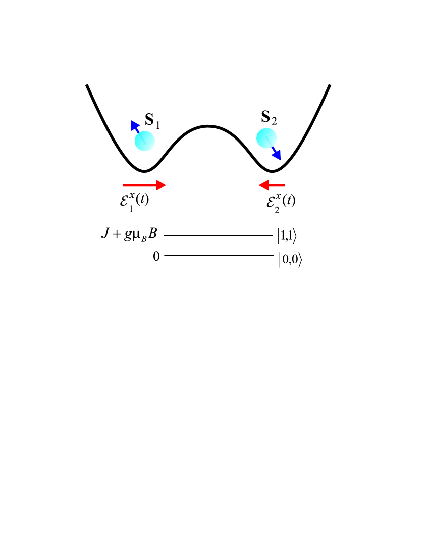
Figure 1: (color online.) Schematic diagram of a two-electron double quantum dot in the presence of the external electric fields.

Here $j=1,2$ represent the electrons $1$ and the electron $2$. $\bm{S}_{j}=\bm{\sigma}_{j}/2$, are the spin operators of two electrons. The Zeeman term $\Delta_{j}=g\mu_{B}B_{j}$, where $\mu_{B}=\hbar|e|/(2m_{0}c)$ is the Bohr magneton, $g$ is the Landé factor with negative value ($g<0$), like in GaAs and InAs, and $m_{0}$ is the mass of the free electron. $B_{1}$ and $B_{2}$ are the static magnetic fields applied to the electron $1$ and $2$ in $z$ direction, respectively. For simplicity, we set $B_{1}=B_{2}=B$, so that $\Delta=\Delta_{1}=\Delta_{2}=g\mu_{B}B$. In the presence of the applied magnetic field, the lowest four eigenstates of the system can be expressed by singlet and triplet for $S=0$ and $S=1$ in the basis of $|S,S_{z}{\rangle}$. If the energy difference between the singlet $|0,0{\rangle}$ and the lowest one of the triplet $|1,1{\rangle}$ is much less than the gap between the singlet and the triplet $J$, which means $|J+\Delta|\ll J$, we focus on the state transition between these lowest two states $|0,0{\rangle}$ and $|1,1{\rangle}$, as shown in Fig. 1. By choosing $|0,0{\rangle}=(1,0)^{T}$ and $|1,1{\rangle}=(0,1)^{T}$, we can write the reduced Hamiltonian $H_{s}$ in the form of $2\times 2$ matrix,

$$H_{\textrm{s}}=\left(\begin{array}[]{cc}-\displaystyle{\frac{3}{4}}J&0\\ 0&\displaystyle{\frac{1}{4}}J+\Delta\end{array}\right).$$ (4)

The interactions between the electric field and the electron $H_{\textrm{int}}$ are expressed as,

$$H_{\textrm{int}}=-\frac{e}{c}\sum_{j}\textbf{A}_{j}\cdot\textbf{v}_{j},$$ (5)

where the vector potential $\textbf{A}_{j}(t)$ are related to the external electric fields, ${\bf\mathcal{E}}_{1}(t)=-(1/c)\partial\textbf{A}_{1}/\partial t$ and ${\bf\mathcal{E}}_{2}(t)=-(1/c)\partial\textbf{A}_{2}/\partial t$, and $\textbf{v}_{j}$ are the spin-dependent velocity operators. We consider the SO coupling including structure-related Rashba ($\alpha$) term and bulk-originated Dresselhaus ($\beta$) term for $[110]$ growth axis,

$$H_{\textrm{soc}}=\sum_{j}\alpha(\sigma^{x}_{j}p^{y}_{j}-\sigma^{y}_{j}p^{x}_{j})+\sum_{j}\beta\sigma^{z}_{j}p^{x}_{j},$$ (6)

so that the spin-dependent velocity operators become

$$v^{x}_{j} = \frac{i}{\hbar}\left[H_{\rm soc},x_{j}\right]=\beta\sigma^{z}_{j}-\alpha\sigma^{y}_{j},$$ (7)

$$v^{y}_{j} = \frac{i}{\hbar}\left[H_{\rm soc},y_{j}\right]=\alpha\sigma^{x}_{j}.$$ (8)

Therefore, the total spin-dependent Hamiltonian $H_{\textrm{total}}$ is

$$H_{\textrm{total}}=\frac{\hbar}{2}\left(\begin{array}[]{cc}Z_{1}&X+iY\\ X-iY&Z_{2}\end{array}\right).$$ (11)

where

$$X = \frac{\sqrt{2}\alpha}{\hbar}\frac{e}{c}(A^{y}_{1}-A^{y}_{2}),$$ (12)

$$Y = -\frac{\sqrt{2}\alpha}{\hbar}\frac{e}{c}(A^{x}_{1}-A^{x}_{2}),$$ (13)

$$Z_{1} = -\frac{3J}{2\hbar},$$ (14)

$$Z_{2} = \frac{1}{\hbar}\left[\frac{J}{2}+2\Delta-2\frac{e}{c}\beta(A^{x}_{1}+A^{x}_{2})\right].$$ (15)

To rewrite the symmetric Hamiltonian, we shift one quantity $Z_{0}=-J/4+\Delta/2-(e\beta/2c)(A^{x}_{1}+A^{x}_{2})$, and finally obtain Hamiltonian $H_{\textrm{total}}=Z_{0}\hat{I}+H$, where

$$H=\frac{\hbar}{2}\left(\begin{array}[]{cc}Z&X+iY\\ X-iY&-Z\end{array}\right),$$ (18)

with $Z=(1/\hbar)\left[-J-\Delta+(e\beta/c)(A^{x}_{1}+A^{x}_{2})\right]$. The solution to the Schrödinger equation of $H$ differentiates from that of $H_{\textrm{total}}$ by the factor $\exp[-i\int Z_{0}(t^{\prime})dt^{\prime}]$, while the energy level $|0,0{\rangle}$ and $|1,1{\rangle}$ are shifted by $Z_{0}$. The states after the shifting are denoted by $|1{\rangle}$ and $|-1{\rangle}$, respectively, and their populations remain unchanged as the ones of the previous states, $|0,0{\rangle}$ and $|1,1{\rangle}$.

Transitionless fast spin tranfer— Our aim is to transfer the spin from $|-1{\rangle}$ to $|1{\rangle}$ totally during a reasonably short time duration. The form of Hamiltonian $H$ in Eq. 18 tells us that $Y$ and $Z$ are the functions of $A^{x}_{1}$ and $A^{x}_{2}$ and $X$ is the function of $A^{y}_{1}$ and $A^{y}_{2}$. Different from the Hamiltonian of one electron confined in a single dot single-dot , the transitionless quantum driving can be applicable to the spin control in a two-electron double QD, as we can figure out how the Hamiltonian $H$ (including reference Hamiltonian $H_{0}$ and counter-diabatic term $H_{1}$) is implemented by corresponding electric fields. We may take the reference Hamiltonian $H_{0}$ as

$$H_{0}=\frac{\hbar}{2}\left(\begin{array}[]{cc}Z&iY\\ -iY&-Z\end{array}\right),$$ (21)

driven by $A^{x}_{1}$ and $A^{x}_{2}$. The example of a double QD of GaAs-based structure is considered below, where $g=-0.44$ and the static magnetic fields are $B_{1}=B_{2}=3.43$ T. The energy gap between the singlet and the triplet is $J=0.1$ meV, so that $|J+\Delta|/J=0.12\ll 1$ with the above parameters.

With the help of reference Hamiltonian (21), we can write down the instantaneous eigenstates, $|\chi_{\pm}{\rangle}$, satisfying $H_{0}|\chi_{\pm}{\rangle}=E_{\pm}|\chi_{\pm}{\rangle}$, where the instantaneous eigenvalues are $E_{\pm}=\pm\hbar\sqrt{Z^{2}+Y^{2}}/2$, and the instantaneous eigenstates are

$$|\chi_{+}{\rangle}=\left(\begin{array}[]{c}\cos\displaystyle{\frac{\theta}{2}}e^{i\varphi}\\ \sin\displaystyle{\frac{\theta}{2}}\end{array}\right),|\chi_{-}{\rangle}=\left(\begin{array}[]{c}\sin\displaystyle{\frac{\theta}{2}}\\ -\cos\displaystyle{\frac{\theta}{2}}e^{-i\varphi}\end{array}\right),~{}~{}~{}~{}~{}$$ (26)

with the mixing angle $\theta=\arccos[Z/(Y^{2}+Z^{2})]$ and $\varphi=\pi/2$. Once the adiabaticity condition Berry09 ; ChenPRA

$$\left|\frac{Z\dot{Y}-Y\dot{Z}}{(Y^{2}+Z^{2})^{\frac{3}{2}}}\right|\ll 1$$ (27)

is fulfilled, the state $|\Psi^{0}{\rangle}$, the solution to the Schrödinger equation of $H_{0}$, evolves from $|\Psi^{0}(0){\rangle}=|\chi_{\pm}(0){\rangle}$ and follows the adiabatic approximation

$$|\Psi^{0}(t){\rangle}=\exp\left[-\frac{i}{\hbar}\int^{t}_{0}dt^{\prime}E_{\pm}(t^{\prime})\right]|\chi_{\pm}(t){\rangle}.$$ (28)

Otherwise, transitions between $|\chi_{\pm}(0){\rangle}$ will occur. To implement population inversion, from $|-1{\rangle}$ to $|1{\rangle}$, along one of instantaneous eigenstate, $|\chi_{+}(t){\rangle}$, we set the ansatz of the vector potential $A^{x}_{j}=A_{0}\tanh[(t-a_{j}t_{f})/(w_{j}t_{f})]$, where $a_{j}$, $w_{j}$ describe the change rate of $A^{x}_{j}$ and $j=1,2$. To fulfill the initial and final states, $Y(0)=Y(t_{f})=0$ should be fixed, which means at the initial and final times $A^{x}_{1}$ and $A^{x}_{2}$ are equal to each other. Meanwhile, the mixing angle $\theta$ goes from $\pi$ to $0$, crossing the point $\pi/2$ during the interval $(0,t_{f})$. With this strategy, we produce the reference electric fields $\mathcal{E}^{x}_{j}$, displayed in Fig. 2 (c). For the following comparison, we first show the dynamics of populations for the instantaneous eigenstates, $P^{\textrm{in}}_{1}(t)=|{\langle}1|\chi_{+}(t){\rangle}|^{2}$ and $P^{\textrm{in}}_{-1}(t)=|{\langle}-1|\chi_{+}(t){\rangle}|^{2}$ (seen in Fig. 2(a)). In practice, this process is not adiabatic, so the populations of exact solution, $\Psi^{0}(t)$, of Hamiltonian $H_{0}$ are obtained as $P_{1}^{0}(t_{f})=|{\langle}1|\Psi^{0}(t_{f}){\rangle}|^{2}=0.76$ and $P_{-1}^{0}(t_{f})=|{\langle}-1|\Psi^{0}(t_{f}){\rangle}|^{2}=0.24$, (seen in Fig. 2(b)), which are not consistent with that of the instantaneous eigenstates. Of course, the adiabatic passage can be realized by extending $t_{f}$ and increasing the electric fields, respectively. For example, if we prolong $t_{f}=14$ ns and keep the previous $A^{x}_{j}$, the process will become adiabatic, and $P_{1}^{0}(t_{f})=0.9999$ is finally achieved. On the other hand, $P_{1}^{0}(t_{f})=0.9999$ can be also achieved, when the magnitude of ${\mathcal{E}^{x}_{j}}$ are increased by $11.5$ V/ m and keep $t_{f}=2$ ns.

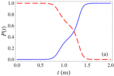
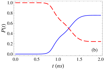
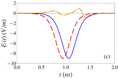
Figure 2: (color online.) (a) Time evolution of the populations $P_{1}^{\textrm{in}}(t)$ (solid blue line) and $P_{-1}^{\textrm{in}}(t)$ (dashed red line) as the instantaneous eigenstates of $H_{0}$, which coincide with the populations $P_{1}(t)$ and $P_{-1}(t)$ as the solution to the Schrödinger equation of $H$. (b) Time evolution of the populations $P_{1}^{0}(t)$ (solid blue line) and $P_{-1}^{0}(t)$ (dashed red line) as the solution to the Schrödinger equation of $H_{0}$, showing that this is not an adiabatic process. (c) The applied electric fields in the $x$ direction ${\mathcal{E}}^{x}_{1}$ (solid blue line) and ${\mathcal{E}}^{x}_{2}$ (dashed red line), and the additional two electric fields in the $y$ direction with the difference ${\mathcal{E}}^{y}_{D}={\mathcal{E}}^{y}_{1}-{\mathcal{E}}^{y}_{2}$ (dot-dashed orange line) drive the population inversion. Other Parameters: $t_{f}=2$ ns, $\hbar\alpha=1.2\times 10^{-6}$ meV $\cdot$ cm, $\hbar\beta=0.3\times 10^{-6}$ meV $\cdot$ cm.

Next, transitionless quantum driving will provide supplementary time-dependent interactions $H_{1}$ that cancel the diabatic couplings of a reference process $H_{0}$, and make the reference process fast and adiabatic-like. The supplementary counter-diabatic term $H_{1}=\sum_{\pm}|\partial_{t}\chi_{\pm}{\rangle}{\langle}\chi_{\pm}|$ is Berry09 ; Chen10b

$$H_{1}=\frac{\hbar}{2}\left(\begin{array}[]{cc}0&X\\ X&0\end{array}\right),$$ (31)

driven by $A^{y}_{1}$ and $A^{y}_{2}$, where $X=\dot{\theta}=(\dot{Y}Z-Y\dot{Z})/(Z^{2}+Y^{2})$. As a result, the solution $\Psi(t)$ to the Schrödinger equation of $H=H_{0}+H_{1}$ becomes exactly the adiabatic approximation of $H_{0}$. The corresponding dynamics of the populations, $P_{1}(t)=|{\langle}1|\Psi(t){\rangle}|^{2}$ and $P_{-1}(t)=|{\langle}-1|\Psi(t){\rangle}|^{2}$. The populations $P_{1}(t)$ and $P_{2}(t)$ coincide with $P_{1}^{\textrm{in}}(t)$ and $P_{2}^{\textrm{in}}(t)$ respectively, as shown in Fig. 2(a). The difference between two additional $y$ components is $A^{y}_{D}=A^{y}_{1}-A^{y}_{2}=\hbar\dot{\theta}/(\sqrt{2}e\alpha)$ and the corresponding time-dependent function of ${\mathcal{E}}^{y}_{D}={\mathcal{E}}^{y}_{1}-{\mathcal{E}}^{y}_{2}$ is plotted in Fig. 2(c). The maximal magnitudes of ${\mathcal{E}}^{y}_{D}$ is $0.94$ V/m. Obviously, they are much less than the increasing values in magnitude of ${\mathcal{E}}^{x}_{j}$ to achieve the adiabatic process, as mentioned above. This implies that the transitionless quantum driving can really speed up the adiabatic process. As a matter of fact, ${\mathcal{E}}^{y}_{D}$, as the function of $\dot{\theta}$, is related to $\dot{Y}$ and $\dot{Z}$. The shorter time is, the larger value of ${\mathcal{E}}^{y}_{D}$ is required. To implement ${\mathcal{E}}^{y}_{D}$ easily in the experiment, we need the smooth function of ${\mathcal{E}}^{y}_{D}$, therefore in general ${\mathcal{E}}^{x}_{1}$ and ${\mathcal{E}}^{x}_{2}$ should not vary very dramatically.

$z$-axis rotation— In reality, the electron spin is subject to the device-dependent noise, which could be the amplitude noise of the electric fields single-dot . It can be quite important, especially when the electric fields are relatively weak. From the above analysis, we find that four controllable parameters, ${\mathcal{E}}^{x}_{j}$ and ${\mathcal{E}}^{y}_{j}$, $x$ and $y$ components of the electric fields for each electron in double QD should be applied. If $y$ component of the electric fields can be reduced, we can decrease decoherent effects resulting from the device-dependent noise. To this end, we can apply the concept of multiple Schrödinger pictures, and make unitary transformation of Hamiltonian $H$ by $z$-axis rotation Multiple-picture . We write down the dynamical Hamiltonian as follows

$$H=\frac{\hbar}{2}\left(\begin{array}[]{cc}Z&iQe^{i(\phi-\pi/2)}\\ -iQe^{-i(\phi-\pi/2)}&-Z\end{array}\right),$$ (34)

where $\tan\phi=Y/X$ and $Q=\sqrt{X^{2}+Y^{2}}$.

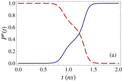
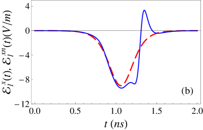
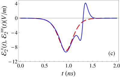
Figure 3: (color online.) (a) The populations $P^{n}_{1}(t)$ and $P^{n}_{-1}(t)$ as the solution to the Schrödinger equation $H^{\prime}$. (b) Comparisons between ${\mathcal{E}}^{xn}_{1}$ (solid blue line) and ${\mathcal{E}}^{x}_{1}$ (dashed red line). (c) Comparisons between ${\mathcal{E}}^{xn}_{2}$ (solid blue line) and ${\mathcal{E}}^{x}_{2}$ (dashed red line). Other parameters are the same as in Fig. 2.

By applying the unitary transformation Berry90

$$U=\frac{\hbar}{2}\left(\begin{array}[]{cc}e^{i(\phi-\pi/2)}&0\\ 0&e^{-i(\phi-\pi/2)}\end{array}\right),$$ (37)

which amounts to a rotation around $z$ axis by the angle $\pi/2-\phi$, we calculate the new Hamiltonian $H^{\prime}=U^{\dagger}(H-K)U$ with $K=i\hbar\dot{U}U^{\dagger}$, and finally obtain

$$H^{\prime}=\frac{\hbar}{2}\left(\begin{array}[]{cc}Z+\dot{\phi}&iQ\\ -iQ&-Z-\dot{\phi}\end{array}\right),$$ (40)

without $\sigma_{x}$ term. We should notice that the dynamics of Hamiltonian $H=H_{0}+H_{1}$ and $H^{\prime}$ is not the same (the populations are the same because of $z$ rotation). However, the Hamiltonian $H^{\prime}$ is equal to the original one $H=H_{0}+H_{1}$ at $t=0$ and $t_{f}$, which guarantees that the initial (final) states of $H$ and $H^{\prime}$ coincide. So the Hamiltonian $H^{\prime}$ can provide an alternative way to implement the shortcuts to adiabaticity. According to the Hamiltonian $H^{\prime}$ Eq. (40), we may acquire two new controllable parameters, $\mathcal{E}^{xn}_{1}$ and $\mathcal{E}^{xn}_{2}$, $x$ component of the electric fields, since $Z+\dot{\phi}$ and $Q$ are the functions of the sum and the difference of $A^{xn}_{1}$ and $A^{xn}_{2}$, respectively. The solution, $\Psi^{n}(t)$, of the Schrödinger equation of $H^{\prime}$ can be solved numerically, and the populations $P^{n}_{1}(t)=|{\langle}1|\Psi^{n}(t){\rangle}|^{2}$ and $P^{n}_{-1}(t)=|{\langle}-1|\Psi^{n}(t){\rangle}|^{2}$, are shown in Fig. 3 (a). At the final time, $P_{1}^{n}(t_{f})=1$ and the population is completely inverted. The new electric fields only in $x$ direction are shown in Fig. 3 (b-c) with some corrections compared with the previous ones ${\mathcal{E}}^{x}_{1}$ and ${\mathcal{E}}^{x}_{2}$.

Conclusion— We propose the shortcuts to manipulate the spin states formed in a two-election double QD by using transitionless quantum driving. The Hamiltonian $H$ is divided into two parts, the reference process $H_{0}$, driven by $A^{x}_{1}$ and $A^{x}_{2}$, and the supplementary time-dependent interaction $H_{1}$, driven by $A^{y}_{1}$ and $A^{y}_{2}$. By applying $x$ and $y$ components of electric fields for each electron, the spin system follows exactly the adiabatic approximation of the reference Hamiltonian $H_{0}$, in the time scale of nanosecond. In order to simplify the setup, and decrease the device-dependent noise effect, we further transform the Hamiltonian by $z$ axis and obtain the new Hamiltonian implemented only by $x$ component of electric fields. This provides an alternative shortcut to realize the fast and adiabatic-like spin control. We hope these results may lead to the applications in spintronics and quantum information processing with the state-of-the-art technique.

Acknowledgement— Y. B. acknowledges financial support from the Basque Government (Grant Nos. BFI-2010-255 and IT472-10), Ministerio de Ciencia e Innovacion (Grant No. FIS2009-12773-C02-01), and the UPV/EHU under program UFI 11/55. Valuable discussions from E. Ya. Sherman and X. Chen are appreciated.

References

(1) F. H. L. Koppens, C. Buizert, K. J. Tielrooij, I. T. Vink, K. C. Nowack, T. Meunier, L. P. Kouwenhoven, and L. M. K. Vandersypen, Nature 442, 766 (2006).
(2) E. I. Rashba, Phys. Rev. B 78, 195302 (2008); E. I. Rashba and Al. L. Efros, Phys. Rev. Lett. 91, 126405 (2003).
(3) K. C. Nowack, F. H. L. Koppens, Yu. V. Nazarov, L. M. K. Vandersypen, Science 318, 1430 (2007).
(4) X. Chen, A. Ruschhaupt, S. Schmidt, A. del Campo, D. Guéry-Odelin, and J. G. Muga, Phys. Rev. Lett. 104, 063002 (2010).
(5) M. V. Berry, J. Phys. A 42, 365303 (2009).
(6) M. Demirplak and S. A. Rice, J. Phys. Chem. A 107, 9937 (2003); J. Phys. Chem. B 109, 6838 (2005); J. Chem. Phys. 129, 154111 (2008).
(7) X. Chen, I. Lizuain, A. Ruschhaupt, D. Guéry-Odelin, and J. G. Muga, Phys. Rev. Lett. 105, 123003 (2010).
(8) X. Chen, E. Torrontegui, and J. G. Muga, Phys. Rev. A 83, 062116 (2011).
(9) Y. Ban, X. Chen, E. Ya. Sherman and J. G. Muga, Phys. Rev. Lett. 109, 206602 (2012).
(10) Y. Ban, X. Chen, E. Ya. Sherman and J. G. Muga, unpublished (2012).
(11) K. Takahashi, arXiv:1209.3153 (2012).
(12) M. G. Bason, M. Viteau, N. Malossi, P. Huillery, E. Arimondo, D. Ciampini, R. Fazio, V. Giovannetti, R. Mannella, and O. Morsch, Nat. Phys. 8, 147 (2012).
(13) J.-F. Zhang, J. H. Shim, I. Niemeyer, T. Taniguchi, T. Teraji, H. Abe, S. Onoda, T. Yamamoto, T. Ohshima, J. Isoya, and D. Suter,
arXiv:1212.0832.
(14) S. Ibañes, X. Chen, E. Torreontegui, J. G. Muga and A. Ruschhaupt, Phys. Rev. Lett. 109, 100403 (2012).
(15)H. R. Lewis and W. B. Riesenfeld, J. Math. Phys. 10, 1458 (1969).