Compute and Forward: End to End Performance over Residue Class Based Signal Constellation

Abstract

In this letter, the problem of implementing compute and forward (CF) is addressed. We present a practical signal model to implement CF which is built on the basis of Gaussian integer lattice partitions. We provide practical decoding functions at both relay and destination nodes thereby providing a framework for complete analysis of CF. Our main result is the analytical derivation and simulations based validation of union bound of probability of error for end to end performance of CF. We show that the performance is not limited by the linear combination decoding at the relay but by the full rank requirement of the coefficient matrix at the destination.

I Introduction

In wireless networks with multiple users, relaying is an important technique adopted to maximize the network throughput. In [1], Nazer and Gastpar proposed a novel strategy of generalized relaying called Compute and Forward (CF) which enables the relays in any Gaussian wireless network to decode linear equations of the transmitted symbols with finite field coefficients, using the noisy linear combinations provided by the channel. The linear equations in finite field are transmitted to the destination and upon receiving sufficient linear equations, the destination can decode desired symbols. Further, information theoretical tools are used in [1] to obtain the achievable rate regions. An algebraic approach to implement CF has been introduced in [2] where the authors propose to implement CF making a connection between CF and isomorphism in module theory.

The main contribution of this correspondence is to demonstrate the implementation of CF using practical signal constellations and study its end to end performance from source to destination. We use signal constellations based on one dimensional Gaussian integer lattices to implement CF. We utilize the natural isomorphism existing between these signal constellations and finite fields ([3, 5]) and apply it to design practical encoding and decoding functions at each node of the system from source to destination. In order to understand the factors affecting the CF behavior, we consider integral channels. Therefore, we bypass the errors introduced due to non-integral nature of the channel thereby avoiding the “self-noise” [1]. We show that at high SNR, the overall performance of CF is determined primarily by the choice of the finite field used and is not limited by the detection of linear combinations at the relay. We also provide a tight union bound estimate of probability of error at the destination of CF.

II Preliminaries : Gaussian Integers

In this section, we will present some useful algebraic preliminaries relevant to this letter. Details can be found in [3, 5].

Let $\mathcal{G}$ be the Gaussian Integers $\mathbb{Z}[i]$ and let $\mathcal{G}_{\pi}$ denote the residue class $\mathcal{G}$ modulo $\pi$ where $\pi\in\mathcal{G}$. Any element of $\mathcal{G}$ can be mapped to the residue class $\mathcal{G}_{\pi}$ using the function $\mu:\mathcal{G}\rightarrow\mathcal{G}_{\pi}$. which is defined as

$$\mu(g)=g-\left[\frac{g.\pi^{*}}{\pi.\pi^{*}}\right].\pi$$ (1)

where $\pi^{*}$ is the conjugate of $\pi$, and $\left[.\right]$ is the rounding operation which is defined on complex numbers as $\left[a+bi\right]=\left[a\right]+\left[b\right]i$. The analogy of $\mathcal{G}$ and $\mathcal{G}_{\pi}$ in integer domain is $\mathbb{Z}$ and $\mathbb{Z}_{p}$ for some modulo residue class $\mathbb{Z}\textrm{ mod }p$.

The Gaussian primes are the primes in Gaussian integers which are given by (i) $\pm 1$ and $\pm i$, (ii) the rational primes $p$ with $p\equiv 3\textrm{ mod }4$ and (iii) the factors $a+ib$ of rational primes $p$ with $p\equiv 1\textrm{ mod }4$. The Gaussian primes of type (iii) exist for every $p\equiv 1\textrm{ mod }4$ because the rational primes of type $p\equiv 1\textrm{ mod }4$ can be written as sum of squares $a^{2}+b^{2}$ by the well known Fermat’s Theorem [5, Pg. 291]. Therefore,

$$p=a^{2}+b^{2}=(a+bi)(a-bi)$$

In this letter, we focus on Gaussian primes of type (iii), although extension of this work to other types is straight forward.

III System Model

Consider the CF system model with $L$ sources, a relay and a destination as shown in figure 1. Let $w_{l}\in\mathbb{F}_{p}$ be the message to be transmitted by the $l$-th source ($l=1,2\ldots L$) chosen from a finite field $\mathbb{F}_{p}$ of order $p$. The vector of all the source messages is given by $\mathbf{w}=[\begin{array}[]{ccc}w_{1}&\ldots&w_{L}\end{array}]$. Each source encodes the message $w_{l}$ into a complex signal constellation point using the encoder $\mathcal{E}:\mathbb{F}_{p}\rightarrow\mathbb{C}$ to obtain

$$x_{l}=\mathcal{E}(w_{l})$$ (2)

The signals are transmitted across the channel to the relay. In this model, for the primary understanding, we have assumed that the channel gains are Gaussian integers and hence there is no “self-noise” due to approximation of channel by an integer [1]. It is also assumed that channel undergoes slow fading and hence remains constant throughout the transmission of each signal. The signal obtained at the relay is given by

$$y=h_{1}x_{1}+h_{2}x_{2}+\ldots+h_{L}x_{L}+z$$ (3)

where $h_{l}\in\mathcal{G}$ is the channel coefficient between transmitter $l$ and the relay node, $z$ is i.i.d Gaussian noise given by $z\sim\mathcal{CN}(0,\sigma^{2})$. The signal to noise ratio (SNR) is defined as

$$SNR=\frac{E[\parallel x_{l}\parallel^{2}]}{\sigma^{2}}$$ (4)

The aim of the relay is to compute a linear combination of source messages in the original message space $v\in\mathbb{F}_{p}$ given by

$$v=a_{1}w_{1}\oplus a_{2}w_{2}\ldots a_{L}w_{L}$$ (5)

where $a_{l}\in\mathbb{F}_{p}$ are the linear coefficients chosen on the basis of $h_{l}$ and $\oplus$ indicates summation over finite field. The estimate of $v$ obtained at the relay using the decoder $\mathcal{D}_{R}:\mathbb{C}\rightarrow\mathbb{F}_{p}$ is given by

$$\hat{v}=\mathcal{D}_{R}(y)$$ (6)

The estimate of the linear combination $\hat{v}$ is transmitted to the destination. Here we assume this transmission between relay to destination is error free and the linear combination is obtained at the destination exactly as estimated at the relay. The destination obtains $L$ such linear combinations. Therefore, the decoder at the destination is given by $\mathcal{D}_{D}:\left\{\mathbb{F}_{p}\right\}^{L}\rightarrow\left\{\mathbb{F}_{p}\right\}^{L}$ such that

$$\mathbf{\hat{w}}=\mathcal{D}_{D}(\mathbf{\hat{v}})$$

where $\mathbf{\hat{w}}$ is the estimate of the $L$ original source signal vector $\mathbf{w}$ and $\mathbf{\hat{v}}$ is the vector of estimates of the $L$ linear combinations.

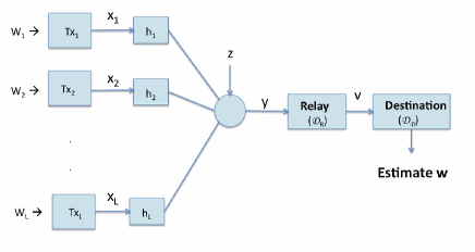
Figure 1: End to End CF System Model

IV Proposed Encoding and Decoding Functions

In this section, we propose the encoding function for the sources and the decoding functions at the relay and the destination in order to implement CF scheme.

IV-A Construction of the Signal Constellation

We define some standard useful functions [3] which we utilize in constructing the signal constellations to implement CF. A signal constellation feasible to implement CF is desired to be isomorphic to a finite field. Therefore, a natural choice is the residue class of Gaussian integers $\mathcal{G}_{\pi}$ because any residue class $\mathcal{G}_{\pi}$ is isomorphic to a finite field $\mathbb{F}_{p}$ if $\pi$ is a prime in $\mathcal{G}$. The size of the field is given by $p=\mid\pi\mid^{2}$. This isomorphism is defined by the bijective function $\varphi:\mathbb{F}_{p}\rightarrow\mathcal{G}_{\pi}$ defined as

$$\varphi(a)=\xi=a-\left[\frac{a.\pi^{*}}{p}\right].\pi$$ (7)

and the inverse $\varphi^{-1}:\mathcal{G}_{\pi}\rightarrow\mathbb{F}_{p}$ given by

$$a=\varphi^{-1}(\xi)=\xi.(v\pi^{*})+\xi^{*}(u\pi^{*})\textrm{ mod }p$$ (8)

where $u.\pi+v\pi^{*}=1$ and the Euclidean algorithm can be applied to calculate $u$ and $v$. With this isomorphism, $\mathcal{G}_{\pi}$ and $\mathbb{F}_{p}$ are mathematically equivalent. In figure 2, some examples of residue class $\mathcal{G}_{\pi}$ along with their finite field mapping are shown. We will now propose the encoding and decoding functions at the sources, relay and destination.

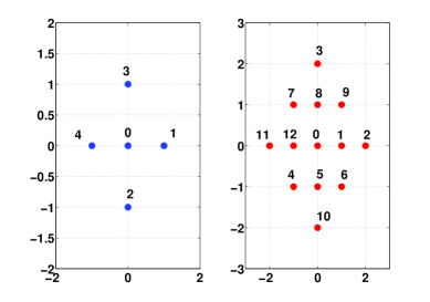
Figure 2: Constellations from residue class $\mathcal{G}_{\pi}$ for $\pi=2+i$ and $\pi=3+2i$ and their respective mapping to finite fields $\mathbb{F}_{5}$ and $\mathbb{F}_{13}$

IV-B Encoding at the source

Let $W$ be the message space which is a finite field comprising of $p$ elements such that $W=\mathbb{F}_{p}$ . The source messages are chosen from the message space $w_{l}\in W$. This message space is required to be isomorphic to some complex signal constellation $S$ in order to implement CF. The encoding at the source is therefore done as follows:

1. Choose a signal space size as $\pi=p^{1/2}$ where $\pi\in\mathcal{G}$. The signal space is hence given by $S=\mathcal{G}_{\pi}$.

2. For each $w_{l}\in W$, obtain the isomorphic element in $\mathcal{G}_{\pi}$ using the bijection function in (7) as $\varphi:W\rightarrow S$ such that

$$x_{l}=\varphi(w_{l})$$

The encoded signals are transmitted to the relay where a noisy linear combination of the signals is obtained given by (3). In the next subsection, we discuss the decoding performed at the relay.

IV-C Decoding at the relay

The relay aims to compute the linear combination $v\in W=\mathbb{F}_{p}$,

$$v=a_{1}w_{1}\oplus a_{2}w_{2}\ldots a_{L}w_{L}$$

where $a_{l}$ is the finite field mapping of the channel gain $h_{l}\in\mathcal{G}$ given by

$$a_{l}=\varphi(\mu(h_{l}))$$ (9)

Particularly, $h_{l}$ is firstly mapped to the residue class $\mathcal{G}_{\pi}$ using the function $\mu$ defined in (1) and then mapped to finite field using $\varphi$ in (7). The decoding process at the relay comprises of the following steps:

1. From the received signal $y$, obtain a maximum likelihood (ML) estimate of $y$

$$\hat{y}_{ML}=\arg\min_{t\in\mathcal{G}}\parallel y-t\parallel^{2}$$ (10)

2. Map the ML estimator output with the corresponding residue class element in $S=\mathcal{G}_{\pi}$ using (1) as

$$\hat{u}=\mu(\hat{y}_{ML})$$ (11)

The output of this operation yields $\hat{u}\in\mathcal{G}_{\pi}$ which is the estimate of linear combination in signal space domain.

3. Map the estimated signal constellation point $\hat{u}$ to message space given by finite field $W=\mathbb{F}_{p}$ using (8) to obtain

$$\hat{v}=\varphi^{-1}(\hat{u})$$ (12)

The output of this operation yields an estimate of the linear combination of the original source signals in finite field $W$.

An error occurs at the relay if the linear combination is incorrectly estimated. More precisely, the probability of error at the relay is

$$P_{R}=\Pr(\hat{v}\neq v)$$ (13)

The relay transmits the estimate of the linear combination to the destination where the original source signals are decoded.

IV-D Decoding at the destination

The destination collects $L$ linear combinations from the relay which can be written as

$$\underbrace{\left[\begin{array}[]{c}\hat{v}^{1}\\ \vdots\\ \hat{v}^{L}\end{array}\right]}_{\hat{\mathbf{v}}}=\underbrace{\left[\begin{array}[]{ccc}a_{1}^{1}&\ldots&a_{L}^{1}\\ \vdots&&\vdots\\ a_{1}^{L}&\ldots&a_{L}^{L}\end{array}\right]}_{\mathbf{A}}\underbrace{\left[\begin{array}[]{c}w_{1}\\ \vdots\\ w_{L}\end{array}\right]}_{\mathbf{w}}$$ (14)

where $\hat{v}^{t}$ denotes the $t-$th linear combination ($t=1\ldots L$) and $a_{l}^{t}$ denotes the $l-$th coefficient in $t-$th linear combination between the $l$th source and relay given by (9). The decoder at the destination inverts the matrix $\mathbf{A}$ and obtains an estimate of $\mathbf{w}$. Therefore,

$$\mathbf{\hat{w}}=\mathbf{A^{-1}}\hat{\mathbf{v}}$$

Note that here the inverse of $\mathbf{A}$ is taken in $\mathbb{F}_{p}$ and $\mathbf{A}$ is required to be full rank in $\mathbb{F}_{p}$ for successful decoding.

The probability of error at the destination is given by

$$P_{D}=\Pr(\mathbf{\hat{w}}\neq\mathbf{w})$$ (15)

Therefore, an error occurs at the destination if the original signals are incorrectly estimated.

V Probability of Error

In this section, we derive an analytical expression for probability of error at the destination. Since the probability of error at the destination is also dependent on the probability of error at the relay, therefore, the later is consequently derived.

Recall from equation (15) that the probability of error at the destination is the probability of decoding incorrect original source signals such that $P_{D}=\Pr(\hat{\mathbf{w}}\neq\mathbf{w})$. Therefore, there is an error in detection of $\mathbf{w}$, if there is an error at the relay in computing any of the $L$ linear combinations of original signals or if all the L linear combinations are not independent (and consequently, $\mathbf{A}$ in (14) is not full rank). In the next theorem , we present a theoretical expression for the union bound on the probability of error at the destination.

Theorem 1.

The union bound estimate of probability of error at the destination in CF with L sources using finite field of size p and Gaussian integer residue class based signal constellation is given by

$$P_{D}\leq P_{1}+(LP_{R})$$

where

$$P_{1}=1-\prod_{t=1}^{L}\left(1-\frac{1}{p^{t}}\right)$$

and

$$P_{R}=1-\left(erf\left(\frac{1}{2\sqrt{2}\sigma}\right)\right)$$

such that $\sigma^{2}$ is the variance of additive noise at the relay.

Proof:

An error occurs at the destination if there is an error in detection of any linear combination at the relay node and/or the linear combinations at the destination are not independent (and consequently, $\mathbf{A}$ is not full rank). Therefore, the union bound estimate of probability of error is given by

$$P_{D}\leq P_{1}+\sum_{L}P_{R}$$

where $P_{1}$ is the probability of $\mathbf{A}$ to have a rank failure (in $\mathbb{F}_{p}$) and $P_{R}$ is the probability of error at the relay. It has been proved in [4] that the probability of an $L\times L$ matrix $\mathbf{A}$ over a finite field of size $p$, not being full rank is given by

$$P_{1}=\Pr(\mid\mathbf{A}\mid=0)=1-\prod_{t=1}^{L}\left(1-\frac{1}{p^{t}}\right)$$ (16)

To evaluate the probability of error at the relay, we use the classic notion of estimation of error probability. Recall from equation (13) that the probability of error at the relay is the probability of decoding an incorrect linear combination such that $P_{R}=\Pr(\hat{v}\neq v)$.We rewrite $\hat{v}$ using (10)-(12) as $\hat{v}=\varphi^{-1}(\mu(\hat{y}_{ML})))$. Since the maps $\mu$ and $\varphi$ are discrete, the equation (13) can be written as

$$P_{R}=\Pr(\hat{y}_{ML}\neq(h_{1}x_{1}+h_{2}x_{2}+\ldots h_{L}x_{L}))$$

Since $h_{l}$, $x_{l}$ $\in\mathcal{G}$, therefore, the above expression is reduced to the probability that the added noise exceeds the voronoi region of $\mathcal{G}$. The noise is assumed to have a Gaussian distribution with mean 0 and variance $\sigma^{2}$. Hence,

$$P_{R}=erfc\left(\frac{1}{2\sqrt{2}\sigma}\right)$$ (17)

where $erfc(x)=\frac{2}{\sqrt{\pi}}\intop_{x}^{\infty}e^{-t^{2}}dt$.

Further, the probability of error in decoding $L$ linear combinations at the relay is given by $\sum_{L}P_{R}=LP_{R}$ because all the transmissions are considered independent. Inserting $P_{1}$ and $P_{R}$ in union bound estimate, the result is proved. ∎

It is clear from (16) that the probability of rank failure is dependent on the number of users $L$ and the finite field size $p$ whereas probability of error at the relay (17) is dependent only on the additive noise.

VI Performance Analysis

In this section, we present the simulations to illustrate the performance of the proposed encoding and decoding functions in terms of (i) the probability of error at the relay, which measures error in detecting linear combinations, (ii) the probability of error at the destination, which measures the probability of incorrect detection of original signals. We consider $L=2$ users sending out signals to the destination via relay. We study the performance of our scheme using different residue classes $\mathcal{G}_{\pi}$ and their corresponding finite fields $\mathbb{F}_{p}$. These classes have been listed in Table I giving the residue class, corresponding fields and the $u$ and $v$ values to design the isomorphism $\varphi$ in (7)-(8). Further, we consider uniformly distributed channel gains between all the nodes. For each residue class, we make $L\times 10^{4}$ transmissions from source to destination and the decoding of original signals is done after every $L$ transmissions.

Figure 3 shows the comparison of probability of error with varying SNR. It can be seen that a higher order finite field (or a higher order $\mathcal{G}_{\pi}$) gives a higher probability of error at the relay for the same SNR. This happens because the source of error at the relay is only the additive noise. The impact of this additive noise is determined by packing and a higher order field will have a denser packing as compared to lower order field for same SNR.

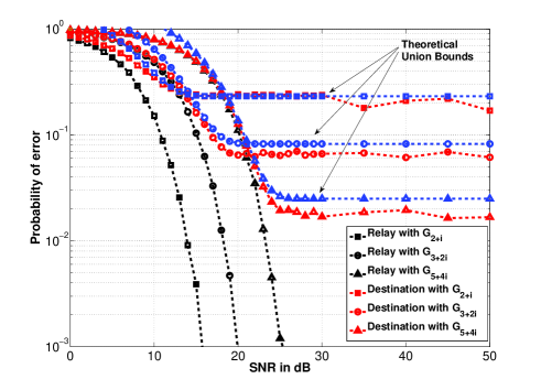
Figure 3: Probability of error at the relay and at the destination. In all cases, $L=2$ users are considered. Three different partitions are plotted.

However, at the destination, the probability of error decreases with increasing SNR up to a certain point and then it attains a constant value. This is because the overall error is contributed not only by the additive noise at the relay but also due to the probability of rank failure at the destination. The probability of rank failure is independent of SNR (16) and is fixed for any given field size and number of users. The probability of error at the destination decreases with increasing SNR only up to the point when it becomes comparable to the probability of rank failure for a given field size. After this point, the error at the relay becomes negligible as compared to error due to rank failure and therefore, error probability at the destination becomes a constant equal to rank failure probability. A higher order partition gives a lower probability of error at the destination at high SNR due to lower probability of rank failure as compared to lower order partition like $\mathcal{G}_{2+i}$. Also, note that the theoretical union bound estimate given in Theorem 1 is reasonably tight.

VII Conclusions

In this letter, we have introduced a concrete scheme to implement Compute and Forward relaying protocol using finite size signal constellations. We have designed encoding and decoding functions using residue class of Gaussian integers and used their natural properties of isomorphism with finite fields to obtain mapping between signal space and message space. We have obtained an analytical union bound estimate of probability of error and validated it via simulations. We proved that at high SNR, full rank requirement of the coefficient matrix plays the key role in determining the end to end performance of CF.

$p$	$\pi$	$u$	$v$
$5$	$2+i$	$-1$	$1+i$
$13$	$3+2i$	$-2$	$1+2i$
$41$	$5+4i$	$-4$	$1+4i$

TABLE I: Finite fields $p$ (where $p\equiv 1\textrm{ mod }$ $4$), $\pi$ (where $p=\pi\pi^{*}$) and the values of $u,v$ (where $u\pi+v\pi^{*}=1$)

References

- [1] B. Nazer & M. Gastpar , “Compute and Forward: Harnessing Interference through Structured Codes”, IEEE Trans. on Info. Theory, vol. 57, no. 10, pp. 6463-6484, Oct 2011.
- [2] C. Feng, D. Silva & F. R. Kschischang, “An Algebraic Approach to Physical Layer Network Coding”, submitted to IEEE Trans. on Info. Theory, 2011.
- [3] K. Huber, “Codes over Gaussian Integers”, IEEE Trans. on Info. Theory, vol. 40, no.1, pp 207-216, Jan.1994
- [4] William. C. Waterhouse, “How often do determinants over finite fields vanish?”, Discrete Mathematics, Volume 65, Issue 1, May 1987, Pages 103-104.
- [5] G. H. Hardy and E. M. Wright, “An Introduction to the theory of Numbers”, Oxford 1979, 5th ed.