Light-Cone Distribution Amplitudes of the Ground State Bottom Baryons in HQET

Abstract

We provide the definition of the complete set of light-cone distribution amplitudes (LCDAs) for the ground state heavy bottom baryons with the spin-parities $J^{P}=1/2^{+}$ and $J^{P}=3/2^{+}$ in the heavy quark limit. We present the renormalization effects on the twist-2 light-cone distribution amplitudes and use the QCD sum rules to compute the moments of twist-2, twist-3, and twist-4 LCDAs. Simple models for the heavy baryon distribution amplitudes are analyzed with account of their scale dependence.

1 Introduction

Precision tests of the unitarity of the quark mixing matrix remain high on the agenda of flavor physics. They allow to pin down the Standard Model (SM) description of CP-violation and may reveal physics beyond the SM (BSM). On the experimental side, the two $B$-meson factories at SLAC and KEK, after approximately a decade of their operation, have made a great impact on the origin of CP-violation in the quark sector of the SM. Especially in $b$ physics, the $B$-factory experiments BABAR and BELLE have concentrated on the production and decays of the $b\bar{b}$ resonances, $\Upsilon(4S)$ and $\Upsilon(5S)$, yielding precise measurements of their decay products, the $B$- and the $\bar{B}$-mesons. Theoretically, inclusive decays of the $B$-mesons, such as the radiative and semileptonic decays, are under quantitative control, thanks to the use of the Heavy Quark Effective Theory (HQET), allowing an expansion in the inverse $b$-quark mass, with perturbative QCD allowing to calculate corrections in $\alpha_{s}(m_{b})$ to each order in $1/m_{b}$. Exclusive semileptonic and radiative decays require, on the other hand, a precise knowledge of the non-perturbative quantities - the decay form factors - to be analyzed precisely. However, also in such cases, the large energy released in the $B\to hX$ decays, where $h$ is a light meson and $X=\gamma,\ell^{+}\ell^{-},\ell^{\pm}\nu_{\ell}$, allows to relate several of these form factors. The resulting large energy effective theory (LEET), which has been replaced by a more systematic effective theory, the Soft Collinear Effective Theory (SCET), has been put to good use in these decays, resulting in a number of theoretical predictions on different observables in various channels, which are found in global agreement with the experimental measurements (see Ref. Buchalla:2008jp for a review).

The attention in flavor physics has so far mostly been focused on the meson sector. Specific processes involving bottom baryons, such as rare decays involving flavor-changing neutral current (FCNC) transitions, are also potential sources of BSM physics. Experiments at the LHC, in particular the LHC$b$, are already analyzing the copiously produced $b$-baryons. As more luminosity is collected, the $b$-baryon sector will become a wider and quantitative field. Theoretically, these decays are more involved, in particular the non-leptonic $b$-baryon decays, but the semileptonic and radiative $b$-baryon decays are tractable. As the starting point for the calculations of the transition form factors, a precise knowledge of the quark distributions inside the baryons is needed. The LCDAs provide this input in the case of light quarks having high virtuality, which then become a crucial input to the calculations of the baryonic transitions in the light cone sum rule approach. Baryonic transitions involving a heavy quark have been studied since the beginning of the 90s. However, the theoretical precision achieved so far is not comparable to the one attained for the corresponding mesonic transitions. So far, most of the heavy baryon distribution amplitudes discussed in the literature Loinaz:1995wz ; Hussain:1990uu are the ones which are motivated by various quark models, which are not manifestly consistent with the QCD constraints. Hence, it is desirable to make theoretical inroads in this sector, guided by QCD. This effort will pay off, as the baryons have the advantage over the $B$-mesons of providing access to spin correlations in various baryon-to-baryon transitions. A full angular analysis of the semileptonic decays of some $b$-baryons, such as the decays of the $\Lambda_{b}$ and the $\Omega_{b}$, will provide a much more detailed view of the underlying dynamics. Of special interest are the semileptonic heavy baryon decays, governed by heavy-to-light form factors. In this retrospect, apart from the theoretical analysis based on the heavy quark effective theory Isgur:1990pm ; Mannel:1990vg ; hep-ph/9701399 , the simplification of baryonic form factors in the large recoil limit is exploited in Refs. Feldmann:2011xf ; Mannel:2011xg (see Ref. Hiller:2001zj ; hep-ph/0702191 ; Wei:2009np for an earlier discussion). In the framework of the soft-collinear effective theory, it is demonstrated that the leading-power heavy-to-light baryonic form factors at large recoil obey the heavy quark and large energy symmetries Wang:2011uv , and in particular the universal function (soft form factor) in $\Lambda_{b}\to\Lambda$ is also calculated within the light-cone QCD sum rules in conjunction with the effective field theory Feldmann:2011xf .

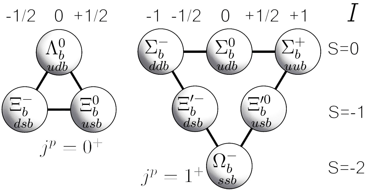
Figure 1: The $SU(3)_{\rm F}$ flavor multiplets of the ground-state bottom baryons. The flavor $SU(3)_{\rm F}$ triplet with the spin-parity $J^{P}=1/2^{+}$ and the scalar light-quark current ($j^{p}=0^{+}$) is shown to the left, and the sextet with the spin-parity $J^{P}=1/2^{+}$ and the vector light-quark current ($j^{p}=1^{+}$) is shown to the right (the similar sextet with $J^{P}=3/2^{+}$ is not presented explicitly). The isospin $I$ and the strangeness $S$ of each baryon state are explicitly specified.

In a pioneering paper Ball:2008fw , the complete classification of three-quark light-cone distribution amplitudes (LCDAs) of the $\Lambda_{b}$-baryon in QCD in the heavy quark limit was given and the scale dependence of the leading-twist LCDA was discussed. In addition, simple models of the LCDAs were suggested and their parameters were fixed based on estimates of the first few moments by the QCD sum rules method. This analysis can be extended to all the ground-state $b$-baryons with both the spin parities $J^{P}=1/2^{+}$ and $J^{P}=3/2^{+}$. The basic steps and some of the results of such an analysis were presented in a conference proceedings Ali:2012zza . In this paper, we provide the details of the calculations, in particular, concerning the $J^{P}=3/2^{+}$ $b$-baryons. Our generalization of the work Ball:2008fw to the full ground state $b$-baryon multiplets provides new input for the eventual calculation of the transition form factors in their decays. In addition, the calculated $SU(3)_{F}$ breaking effects presented here are of interest for studying the strange-quark properties in hadronic background in general. Especially the $\Xi_{b}$-resonances include three different mass quarks, the bottom, the strange and one light $u$- or $d$-quark. They provide interesting insights on the nature of the strange-quark propagating in the QCD background and give some hints on the validity of the quark condensate models. Comparison with the $K$-mesons and the $B_{s}$-meson will show to what extent the condensates are universal quantities.

This paper is organized as follows: We start by discussing the general properties of the single-heavy baryons in the heavy quark limit in Sec. 2, introduce the local interpolating operators of heavy baryons in HQET in Sec. 3, and discuss the non-local light-cone operators of these baryons in Sec. 4. Section 5 is about the renormalization and the scale-dependence of the various matrix elements introduced earlier. The calculations of the correlation functions, which are defined as matrix elements of the non-local and local operators are performed subsequently in Sec. 6 followed by the discussion of our non-perturbative model in Sec.7. Sec. 8 contains our results and numerical analysis, and we conclude with a summary in Sec. 9.

2 Baryon properties in the HQ limit

Baryons with one heavy quark $Q=c,b$ in HQET are classified according to the angular momentum $\ell$ and parity $p$ of the light quark pair, called diquark. The heavy quarks are non-relativistic particles which decouple from the diquark in the leading order of the $1/m_{Q}$ expansion. The ground-state baryons ($\ell=0$) with spin-parity $J^{P}$ are characterized by the spin-parity $j^{p}$ of the diquark. The spins of the light quarks produce two states with $j^{p}=0^{+}$ and $j^{p}=1^{+}$. The spin wave-function is antisymmetric for the state with $j^{p}=0^{+}$, while Fermi statistics of the baryon state and antisymmetry in color space require an antisymmetric flavor wave-function. This results in a baryonic state with isospin $I=0$ constructed from the light $u$- and $d$-quarks and the heavy quark $Q$ which is called the $\Lambda_{Q}$-baryon (the spin-parity is $J^{P}=1/2^{+}$). When the spin-parity of the diquark is $j^{p}=1^{+}$, the spin part of the baryon wave-function is symmetric which requires symmetry of the wave-function in the flavor space. In the case of light $u$- and $d$-quarks beside the heavy quark $Q$, this gives rise to two degenerate states with the isospin $I=1$, which are called $\Sigma_{Q}$- and $\Sigma_{Q}^{*}$-baryons having the spin-parities $J^{P}=1/2^{+}$ and $J^{P}=3/2^{+}$, respectively. Inclusion of the $s$-quark increases the number of heavy baryons in the multiplet which (in addition to the isospin) is characterized by the strangeness $S$. If $S=-1$, there are two baryonic states $\Xi_{Q}$ and $\Xi_{Q}^{\prime}$ with $J^{P}=1/2^{+}$ and $\Xi_{Q}^{*}$-baryon with $J^{P}=3/2^{+}$. For $S=-2$, the baryons with $J^{P}=1/2^{+}$ and $J^{P}=3/2^{+}$ are called $\Omega_{Q}$ and $\Omega_{Q}^{*}$.

The $SU(3)_{\rm F}$ multiplets of the ground-state bottom baryons are shown in Fig. 1. We denote baryons from the triplet and sextet by $H_{b}^{j=0}$ and $H_{b}^{j=1}$, respectively. The corresponding masses of such baryons are presented in Tab. 1 and shown in Fig. 2. The important $\Lambda_{b}\pi$, $\Xi_{b}\pi$ and $\Lambda_{b}K$ thresholds are also specified in the figure. The spectrum of bottom baryons have been enlarged experimentally, substantially thanks to the effort done by the CDF and D0 collaborations at the Tevatron collider during the last several years. In Tab. 1, experimental measurements are taken from Ref. Beringer:1900zz , and we also compare with theoretical predictions (based on HQET Liu:2007fg and Lattice QCD Lewis:2008fu ) for the masses of the ground-state bottom baryons (in units of MeV). Here, $\bar{\Lambda}=m_{H_{b}^{j}}-m_{b}$ and the continuum thresholds $s_{0}$ in HQET for $m_{b}=4.8$ GeV are also given (in units of GeV). The baryons lying below the corresponding strong decay thresholds $\Lambda_{b}\pi$, $\Xi_{b}\pi$ and $\Lambda_{b}K$ are of major importance, since the rare weak decays can be measured without the immense hadronic background.

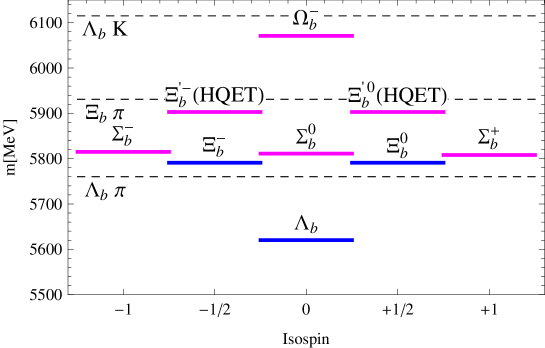
Figure 2: (Color online) Masses and thresholds of the $b$- baryons: $SU_{F}(3)$ triplet consists of $\Lambda_{b}$, $\Xi^{-}_{b}$, and $\Xi^{0}_{b}$ (in blue) and the others belong to the $SU_{F}(3)$ sextet (in magenta). The important hadronic thresholds $\Lambda_{b}\pi$, $\Xi_{b}\pi$ and $\Lambda_{b}K$ are indicated by horizontal dashed lines. The masses are listed in Tab. 1. HQET calculations have been used in the case of lacking experimental input.

The spinor of the baryon from the $j^{p}=0^{+}$ triplet coincides with the spinor $u_{\gamma}$ of the heavy quark. In the case of the baryons from the $j^{p}=1^{+}$ sextets the situation is more complicated. Both the Rarita-Schwinger vector-spinor $R^{\mu}_{\enspace\gamma}(v)$ describing the $J^{P}=3/2^{+}$ baryonic sextet and the spinor of the baryon from the $J^{P}=1/2^{+}$ sextet are specific products of the heavy-quark spinor $u_{\gamma}(v)$ and the polarization vector $\varepsilon^{\mu}(v)$ of the light diquark, in which $v^{\mu}$ is the four-velocity of the heavy baryon. This is the effect of spin decoupling of light and heavy degrees of freedom in the heavy quark limit. The properties of $u_{\gamma}(v)$ and $\varepsilon^{\mu}(v)$ are shortly reviewed below, while detailed information can be found in Falk:1991nq . Subsequently, the baryonic currents are constructed.

The spin and polarization sums are given by

$$\sum\limits_{i=1}^{2}u^{i}(v)\bar{u}^{i}(v) =P_{+}\enspace\enspace\enspace\textnormal{and}\enspace\enspace\enspace\sum\limits_{i=1}^{3}\varepsilon^{*i}_{\mu}(v)\varepsilon^{i}_{\nu}(v)=-g_{\mu\nu}+v_{\mu}v_{\nu},$$ (1)

in which $P_{+}=(1+\not{v})/2$ and the normalization is given by

$$-g^{\mu\nu}\sum\textnormal{Tr}\left[u(v)\varepsilon^{*}_{\mu}(v)\varepsilon_{\nu}(v)\bar{u}(v)\right] =6.$$ (2)

This corresponds to the number of degrees of freedom (3 from the light quark polarization vector, since it has to fulfill the transversality condition $v_{\mu}\varepsilon^{\mu}(v)=0$ leaving 3 degrees of freedom, times 2 from the heavy quark spinor). The polarization vector is normalized as $\varepsilon^{\mu}(v)\varepsilon_{\mu}^{*}(v)=1$.

Table 1: Experimental measurements Beringer:1900zz and theoretical predictions (based on HQET Liu:2007fg and Lattice QCD Lewis:2008fu ) for the masses of the ground-state bottom baryons (in units of MeV). Here, $\bar{\Lambda}=m_{H_{b}^{j}}-m_{b}$ and the continuum thresholds $s_{0}$ in HQET for $m_{b}=4.8$ GeV are also given (in units of GeV).

Baryon	$J^{P}$	Experiment Beringer:1900zz	HQET Liu:2007fg	Lattice QCD Lewis:2008fu	$\bar{\Lambda}$	$s_{0}$
$\Lambda_{b}$	$1/2^{+}$	$5619.4\pm 0.7$	$5637^{+68}_{-56}$	$5641\pm 21^{+15}_{-33}$	0.8	1.2
$\Sigma_{b}^{+}$	$1/2^{+}$	$5811.3\pm 1.9$	$5809^{+82}_{-76}$	$5795\pm 16^{+17}_{-26}$	1.0	1.3
$\Sigma_{b}^{-}$	$1/2^{+}$	$5815.5\pm 1.8$	$5809^{+82}_{-76}$	$5795\pm 16^{+17}_{-26}$	1.0	1.3
$\Sigma_{b}^{*+}$	$3/2^{+}$	$5832.1\pm 1.9$	$5835^{+82}_{-77}$	$5842\pm 26^{+20}_{-18}$	1.0	1.3
$\Sigma_{b}^{*-}$	$3/2^{+}$	$5835.1\pm 1.9$	$5835^{+82}_{-77}$	$5842\pm 26^{+20}_{-18}$	1.0	1.3
$\Xi_{b}^{-}$	$1/2^{+}$	$5791.1\pm 2.2$	$5780^{+73}_{-68}$	$5781\pm 17^{+17}_{-16}$	1.0	1.3
$\Xi_{b}^{0}$	$1/2^{+}$	$5787.8\pm 5.1$	$5780^{+73}_{-68}$	$5781\pm 17^{+17}_{-16}$	1.0	1.3
$\Xi_{b}^{\prime}$	$1/2^{+}$		$5903^{+81}_{-79}$	$5903\pm 12^{+18}_{-19}$	1.1	1.4
$\Xi_{b}^{\prime*}$	$3/2^{+}$		$5903^{+81}_{-79}$	$5950\pm 21^{+19}_{-21}$	1.1	1.4
$\Omega_{b}^{-}$	$1/2^{+}$	$6071\pm 40$	$6036^{+81}_{-81}$	$6006\pm 10^{+20}_{-19}$	1.3	1.5
$\Omega_{b}^{*}$	$3/2^{+}$		$6063^{+83}_{-82}$	$6044\pm 18^{+20}_{-21}$	1.3	1.5

The heavy quark spin has no fixed direction in the heavy quark limit and can be rotated at will. The heavy baryon vector-spinor $\varepsilon^{\mu}(v)u_{\gamma}(v)$ is therefore neither transforming as a spin $3/2$ nor as a spin $1/2$ quantity, since Lorentz invariance is explicitly broken. One has to restore the proper Lorentz-invariant behavior by fixing the heavy quark spinor with respect to the direction of the polarization vector $\varepsilon^{\mu}(v)$. This can be done by using the transformation properties of a spin $3/2$ Rarita-Schwinger vector-spinor $R^{3/2\mu}_{\enspace\enspace\enspace\gamma}(v)$ Falk:1991nq and Grozin:2004yc :

$$(\not{v}R^{3/2\mu}(v))_{\gamma} =R^{3/2\mu}_{\enspace\enspace\enspace\gamma}(v),\enspace\enspace\enspace v_{\mu}R^{3/2\mu}_{\enspace\enspace\enspace\gamma}(v)=0,\enspace\enspace\enspace(\gamma_{\mu}R^{3/2\mu}(v))_{\gamma}=0.$$ (3)

Following Falk:1991nq we define

$$(P_{3/2})_{\enspace\nu\gamma}^{\mu\enspace\enspace\gamma^{\prime}} =\left[\delta_{\nu}^{\mu}-\frac{1}{3}(\gamma^{\mu}+v^{\mu})\gamma_{\nu}\right]_{\gamma}^{\enspace\gamma^{\prime}},$$

$$(P_{1/2})_{\enspace\nu\gamma}^{\mu\enspace\enspace\gamma^{\prime}} =\left[\frac{1}{3}(\gamma^{\mu}+v^{\mu})\gamma_{\nu}\right]_{\gamma}^{\enspace\gamma^{\prime}},$$ (4)

which fulfill the projection operator conditions $P^{2}=P$ and $P_{3/2}+P_{1/2}=\mathds{1}$. Now the product of the spinor $u_{\gamma}(v)$ and the polarization vector $\varepsilon^{\mu}(v)$ can be split in proper spin representations

$$\varepsilon^{\mu}(v)u_{\gamma}(v)=R^{3/2\mu}_{\enspace\enspace\enspace\gamma}(v)+R^{1/2\mu}_{\enspace\enspace\enspace\gamma}(v),$$ (5)

with

$$R^{3/2\mu}_{\enspace\enspace\enspace\gamma}(v) =\left(\left[\varepsilon^{\mu}(v)-\frac{1}{3}(\gamma^{\mu}+v^{\mu})\not{\varepsilon}(v)\right]u(v)\right)_{\gamma},$$

$$R^{1/2\mu}_{\enspace\enspace\enspace\gamma}(v) =\left(\left[\frac{1}{3}(\gamma^{\mu}+v^{\mu})\not{\varepsilon}(v)\right]u(v)\right)_{\gamma}.$$ (6)

A further definition often used is

$$R^{1/2\mu}(v)\equiv\frac{1}{\sqrt{3}}(\gamma^{\mu}+v^{\mu})\gamma_{5}\tilde{R}(v)$$ (7)

with

$$\tilde{R}(v)=\frac{1}{\sqrt{3}}\gamma_{5}\gamma_{\mu}R^{1/2\mu}(v).$$ (8)

One can check that $R^{3/2\mu}_{\enspace\enspace\enspace\gamma}(v)$ fulfills (3), and $R^{1/2\mu}_{\enspace\enspace\enspace\gamma}(v)$ is a spin $1/2$ spinor, with normalization

$$-g_{\mu\nu}\textnormal{Tr}\left[\bar{R}^{3/2\mu}(v)R^{3/2\nu}(v)\right]=4\enspace\enspace\textnormal{and}\enspace\enspace-g_{\mu\nu}\textnormal{Tr}\left[\bar{R}^{1/2\mu}(v)R^{1/2\nu}(v)\right]=-\textnormal{Tr}\left[\bar{\tilde{R}}(v)\tilde{R}(v)\right]=2,$$ (9)

corresponding to (2), where the $3/2$ vector-spinor gets 4 degrees of freedom and the $1/2$ spinor gets 2. One should keep in mind, that this is a global rotation only to get the proper transformation properties. The rotation of the heavy quark spin will not affect the following calculations, which are performed in the heavy quark limit.

3 Local interpolating operators of heavy baryons in HQET

The most general three-quark current of the heavy baryon with one heavy quark in the heavy quark limit is given by the direct product of the diquark, constructed from two light quarks, and the heavy quark field $Q$ due to spin decoupling of the heavy degrees of freedom, discussed in the last section. In this limit, the decay constants $f^{(1)}_{H_{b}^{j=0}}$ and $f^{(2)}_{H_{b}^{j=0}}$ for the $j^{p}=0^{+}$ triplet of bottom baryons are defined by the matrix elements of the local currents Grozin:1992td ; Groote:1997yr :

$$\epsilon^{abc}\langle 0|\left[q_{1}^{aT}(0){\cal C}\gamma_{5}q_{2}^{b}(0)\right]Q_{\gamma}^{c}(0)|H_{b}^{j=0}(v)\rangle=f_{H_{b}^{j=0}}^{(1)}u_{\gamma}(v),$$ (10)

$$\epsilon^{abc}\langle 0|\left[q_{1}^{aT}(0){\cal C}\gamma_{5}v\!\!\!/q_{2}^{b}(0)\right]Q_{\gamma}^{c}(0)|H_{b}^{j=0}(v)\rangle=f_{H_{b}^{j=0}}^{(2)}u_{\gamma}(v).$$ (11)

The decay constants $f^{(1)}_{H_{b}^{j=1}}$ and $f^{(2)}_{H_{b}^{j=1}}$ for the $j^{p}=1^{+}$ bottom baryons are defined as

$$\epsilon^{abc}\langle 0|\left[q_{1}^{aT}(0){\cal C}\gamma_{t}^{\nu}q_{2}^{b}(0)\right]Q_{\gamma}^{c}(0)|H_{b}^{j=1}(v)\rangle=\frac{1}{\sqrt{3}}\,f_{H_{b}^{j=1}}^{(1)}\varepsilon^{\nu}(v)u_{\gamma}(v),$$ (12)

$$\epsilon^{abc}\langle 0|\left[q_{1}^{aT}(0){\cal C}\gamma_{t}^{\nu}v\!\!\!/q_{2}^{b}(0)\right]Q_{\gamma}^{c}(0)|H_{b}^{j=1}(v)\rangle=\frac{1}{\sqrt{3}}\,f_{H_{b}^{j=1}}^{(2)}\varepsilon^{\nu}(v)u_{\gamma}(v),$$ (13)

where $a,\ b,\ c=1,2,3$ are the color indices, $\not{v}=v.\gamma$, $\gamma_{t}^{\mu}=\gamma^{\mu}-\not{v}\,v^{\mu}$, $Q$ is the effective static field of the heavy quark satisfying $\not{v}Q=Q$, the index $T$ indicates a transposition, and ${\cal C}$ is the charge-conjugation matrix with the properties ${\cal C}\gamma_{\mu}^{T}{\cal C}^{-1}=-\gamma_{\mu}$ and ${\cal C}\gamma_{5}{\cal C}^{-1}=\gamma_{5}$. In Eqs. (12) and (13), a factor $1/\sqrt{3}$ is introduced so that the decay constants defined here agree with the ones in Grozin:1992td ; Groote:1997yr . Note that the currents which are commonly used in the literature and define the decay constants, for example the two interpolating currents for the $\Sigma^{*}_{b}$-baryon Groote:1996em

$$J^{\Sigma_{b}^{*}}_{1\mu}(x) =\varepsilon^{abc}\left[q_{1}^{aT}(x){\cal C}\gamma_{t}^{\nu}q_{2}^{b}(x)\right]\left(g_{\mu\nu}-\frac{1}{3}\,\gamma_{t\mu}\gamma_{t\nu}\right)Q^{c}(x),$$ (14)

$$J^{\Sigma_{b}^{*}}_{2\mu}(x) =\varepsilon^{abc}\left[q_{1}^{aT}(x){\cal C}\not{v}\gamma_{t}^{\nu}q_{2}^{b}(x)\right]\left(g_{\mu\nu}-\frac{1}{3}\,\gamma_{t\mu}\gamma_{t\nu}\right)Q^{c}(x),$$ (15)

can be easily derived from the currents defining the matrix elements in (12) and (13) by applying the projectors in (2).

In QCD sum rule calculations of the LCDAs, the time-ordered product of the non-local and local currents (more precisely, the Dirac-conjugated local current) is involved. The most general structure of the Dirac-conjugated $j^{p}=1^{+}$ local interpolating current (for the $j^{p}=0^{+}$ current, see Ball:2008fw ) is now given by the following linear combination:

$$\bar{J}_{\Gamma^{\prime}\gamma}(x)=\varepsilon_{abc}\left[\bar{q}_{1}^{a}(x)\Gamma^{\prime}{\cal C}^{-1}\bar{q}_{2}^{bT}(x)\right]\bar{Q}_{\gamma}^{c}(x),$$ (16)

where $\Gamma^{\prime}=\left(A\mathds{1}+B\not{v}\right)\gamma_{t}^{\mu}$, $B=1-A$, and $A\in[0,1]$. Following Ball:2008fw , the arbitrariness in the choice of the local current, i. e., the variation in $A$, will later be adopted as an error estimate, and we give the results for $A=1/2$, which corresponds to the constituent quark model current that has maximal overlap with the ground-state baryons in the constituent quark model picture, in which all quarks are assumed to be on the mass shell Groote:1997yr .

4 Non-local light-cone operators of heavy baryons in HQET

The currents used in the determination of the LCDAs are by definition non-local objects, aligned along a light-like direction $n^{\mu}$, with coordinates $t_{i}n^{\mu}$ for the $i$-th quark. For simplicity the baryon is defined in the frame of the $b$-quark $Q_{\gamma}=Q_{\gamma}(0)$, and the Wilson lines, which are needed to ensure gauge invariance of the current, are omitted. Their influence will be discussed whenever necessary. Including the light-cone coordinate dependencies one finds for the non-local light-cone operators that they can be written in the heavy quark limit as

$$\left\langle\phantom{H_{b}^{j=1}}\!\!\!\!\!\!\!\!\!\!\!\!\!0\;\right|\left[q_{1}(t_{1}){\cal C}\Gamma^{\mu}q_{2}(t_{2})\right]Q_{\gamma}(0)\left|H_{b}^{j=1}(v)\right\rangle=\frac{1}{\sqrt{3}}f_{H_{b}^{j=1}}\psi^{\Gamma}(t_{1},t_{2})\;\varepsilon^{\mu}(v)u_{\gamma}(v),$$ (17)

where the color indicies are suppressed to simplify the equation as well as the transposition superscript on $q_{1}(t_{1})$. In (17), $\Gamma^{\mu}$ symbolizes all possible spinor structures allowed by the Lorentz symmetry and $\psi^{\Gamma}(t_{1},t_{2})$ are the light-cone distribution amplitudes corresponding to the current defined by $\Gamma^{\mu}$. In total there are at maximum eight linear independent structures, $n^{\mu}\mathds{1}$, $\gamma^{\mu}$, $n^{\mu}\not{v}$, $n^{\mu}\not{n}$, $-i\sigma^{\mu\nu}v_{\nu}$, $-i\sigma^{\mu\nu}n_{\nu}$, $-in^{\mu}\sigma^{\nu\rho}n_{\nu}v_{\rho}$ and $\epsilon^{\mu\nu\rho\tau}v_{\nu}n_{\rho}\gamma_{\tau}\gamma_{5}$ with $\epsilon^{0123}=1$.

Since the quarks are aligned along the light-like direction $n^{\mu}$, it is convenient for the description of the quark dynamics to work in the light-cone basis, where an arbitrary vector $a^{\mu}$ is decomposed as

$$a^{\mu} =\frac{1}{2}\left(a_{-}n^{\mu}+a_{+}\bar{n}^{\mu}\right)+a_{\perp}^{\mu},$$ (18)

in which $n^{\mu}=(1,0,0,-1)$ and $\bar{n}^{\mu}=(1,0,0,1)$ are light-cone vectors with $n^{2}=\bar{n}^{2}=0$, $n_{\mu}\bar{n}^{\mu}=2$, and $a_{\perp}^{\mu}$ refers to the remaining two space-like dimensions, which are perpendicular to both $n^{\mu}$ and $\bar{n}^{\mu}$. The scalar product of two vectors $a^{\mu}$ and $b^{\mu}$ is given by

$$a_{\mu}b^{\mu} =\frac{1}{2}\left(a_{+}b_{-}+a_{-}b_{+}\right)+a_{\perp\mu}b_{\perp}^{\mu}.$$ (19)

The coefficients of the decomposed kinematical vectors

$$v^{\mu} =\frac{1}{2}\left(\frac{n^{\mu}}{v_{+}}+v_{+}\bar{n}^{\mu}\right),$$ (20)

$$\varepsilon^{\mu}(v) =\frac{e}{2}\left(\frac{n^{\mu}}{v_{+}}-v_{+}\bar{n}^{\mu}\right)+\varepsilon_{\perp}^{\mu}(v),$$ (21)

have been chosen in a way to fulfill the conditions $v^{2}=1$, $\varepsilon^{\mu}(v)\varepsilon_{\mu}(v)=-1$ and the transversality condition $v_{\mu}\varepsilon^{\mu}(v)=0$. The light-like vertors are chosen in a way that $v^{\mu}$ has no perpendicular components. Accordingly, $\varepsilon_{\perp}^{\mu}(v)$ and $\varepsilon_{\parallel}^{\mu}(v)\equiv\varepsilon^{\mu}(v)-\varepsilon_{\perp}^{\mu}(v)$ are called transverse and parallel polarizations, respectively. They fulfill the conditions $\varepsilon_{\parallel\mu}(v)\varepsilon_{\perp}^{\mu}(v)=0$, $\varepsilon_{\parallel\mu}(v)\varepsilon_{\parallel}^{\mu}(v)=-e^{2}$, $\varepsilon_{\perp\mu}(v)\varepsilon_{\perp}^{\mu}(v)=e^{2}-1$ and $n_{\mu}\varepsilon^{\mu}(v)=-ev_{+}$ (in the following, the reference of the polarization vector and its components to the four-velocity $v$ will be understood implicitly). The scalar variable $e$ is the measure for the amount of the diquark parallel polarization. Note that the index $\perp$ refers to being perpendicular to both vectors $n^{\mu}$ and $\bar{n}^{\mu}$ (and also the four-velocity $v^{\mu}$), while the index $t$ refers to being perpendicular to $v^{\mu}$ only. The vector

$$\bar{v}^{\mu}=\frac{1}{2}\left(\frac{n^{\mu}}{v_{+}}-v_{+}\bar{n}^{\mu}\right)$$ (22)

is the only possible normalized combination ($\bar{v}^{2}=-1$) of $n^{\mu}$ and $\bar{n}^{\mu}$ which fulfills the transversality condition $v_{\mu}\bar{v}^{\mu}=0$. In this notation, the parallel polarization vector is simply given by $\varepsilon_{\parallel}^{\mu}=e\,\bar{v}^{\mu}$.

For comparison, let us recall the set of the non-local currents for the spin-parity $j^{p}=0^{+}$ diquark and the corresponding LCDAs given in Ball:2008fw with $\{\psi^{n},\,\psi^{n\bar{n}},\,\psi^{\mathds{1}},\,\psi^{\bar{n}}\}$ corresponding to $\{\Psi_{2},\,\Psi_{3}^{\sigma},\,\Psi_{3}^{s},\,\Psi_{4}\}$ and a change of the labeling of the decay constants, which are labeled here by the superscript $(1)$ for vector and $(2)$ for tensor currents:

$$\frac{1}{v_{+}}\left\langle\phantom{H_{b}^{j=1}}\!\!\!\!\!\!\!\!\!\!\!\!\!0\;\right|\left[q_{1}(t_{1}){\cal C}\gamma_{5}\not{n}q_{2}(t_{2})\right]Q_{\gamma}\left|H_{b}^{j=0}\right\rangle =\psi^{n}(t_{1},t_{2})\,f^{(1)}_{H_{b}^{j=0}}u_{\gamma},$$

$$\frac{i}{2}\left\langle\phantom{H_{b}^{j=1}}\!\!\!\!\!\!\!\!\!\!\!\!\!0\;\right|\left[q_{1}(t_{1}){\cal C}\gamma_{5}\sigma_{\bar{n}n}q_{2}(t_{2})\right]Q_{\gamma}\left|H_{b}^{j=0}\right\rangle =\psi^{n\bar{n}}(t_{1},t_{2})\,f^{(2)}_{H_{b}^{j=0}}u_{\gamma},$$

$$\left\langle\phantom{H_{b}^{j=1}}\!\!\!\!\!\!\!\!\!\!\!\!\!0\;\right|\left[q_{1}(t_{1}){\cal C}\gamma_{5}q_{2}(t_{2})\right]Q_{\gamma}\left|H_{b}^{j=0}\right\rangle =\psi^{\mathds{1}}(t_{1},t_{2})\,f^{(2)}_{H_{b}^{j=0}}u_{\gamma},$$

$$v_{+}\left\langle\phantom{H_{b}^{j=1}}\!\!\!\!\!\!\!\!\!\!\!\!\!0\;\right|\left[q_{1}(t_{1}){\cal C}\gamma_{5}\not{\bar{n}}q_{2}(t_{2})\right]Q_{\gamma}\left|H_{b}^{j=0}\right\rangle =\psi^{\bar{n}}(t_{1},t_{2})\,f^{(1)}_{H_{b}^{j=0}}u_{\gamma},$$ (23)

where $\sigma_{\bar{n}n}=\sigma_{\mu\nu}\bar{n}^{\mu}n^{\nu}$. In a similar way, we introduce the set of the parallel currents and their LCDAs as follows:

$$\frac{\bar{v}^{\mu}}{v_{+}}\left\langle\phantom{H_{b}^{j=1}}\!\!\!\!\!\!\!\!\!\!\!\!\!0\;\right|\left[q_{1}(t_{1}){\cal C}\not{n}q_{2}(t_{2})\right]Q_{\gamma}\left|H_{b}^{j=1}\right\rangle =\frac{1}{\sqrt{3}}\psi_{\|}^{n}(t_{1},t_{2})\,f^{(1)}_{H_{b}^{j=1}}\,\varepsilon_{\parallel}^{\mu}u_{\gamma},$$

$$\frac{i\bar{v}^{\mu}}{2}\left\langle\phantom{H_{b}^{j=1}}\!\!\!\!\!\!\!\!\!\!\!\!\!0\;\right|\left[q_{1}(t_{1}){\cal C}\sigma_{\bar{n}n}q_{2}(t_{2})\right]Q_{\gamma}\left|H_{b}^{j=1}\right\rangle =\frac{1}{\sqrt{3}}\psi_{\|}^{n\bar{n}}(t_{1},t_{2})\,f^{(2)}_{H_{b}^{j=1}}\,\varepsilon_{\parallel}^{\mu}u_{\gamma},$$

$$\bar{v}^{\mu}\left\langle\phantom{H_{b}^{j=1}}\!\!\!\!\!\!\!\!\!\!\!\!\!0\;\right|\left[q_{1}(t_{1}){\cal C}q_{2}(t_{2})\right]Q_{\gamma}\left|H_{b}^{j=1}\right\rangle =\frac{1}{\sqrt{3}}\psi_{\|}^{\mathds{1}}(t_{1},t_{2})\,f^{(2)}_{H_{b}^{j=1}}\,\varepsilon_{\parallel}^{\mu}u_{\gamma},$$

$$-v_{+}\bar{v}^{\mu}\left\langle\phantom{H_{b}^{j=1}}\!\!\!\!\!\!\!\!\!\!\!\!\!0\;\right|\left[q_{1}(t_{1}){\cal C}\not{\bar{n}}q_{2}(t_{2})\right]Q_{\gamma}\left|H_{b}^{j=1}\right\rangle =\frac{1}{\sqrt{3}}\psi_{\|}^{\bar{n}}(t_{1},t_{2})\,f^{(1)}_{H_{b}^{j=1}}\,\varepsilon_{\parallel}^{\mu}u_{\gamma},$$ (24)

and the set of the transverse currents and LCDAs:

$$\frac{1}{v_{+}}\left\langle\phantom{H_{b}^{j=1}}\!\!\!\!\!\!\!\!\!\!\!\!\!0\;\right|\left[q_{1}(t_{1}){\cal C}\not{n}\gamma_{\perp}^{\mu}q_{2}(t_{2})\right]Q_{\gamma}\left|H_{b}^{j=1}\right\rangle =\frac{1}{\sqrt{3}}\psi_{\perp}^{n}(t_{1},t_{2})\,f^{(2)}_{H_{b}^{j=1}}\,\varepsilon_{\perp}^{\mu}u_{\gamma},$$

$$\left\langle\phantom{H_{b}^{j=1}}\!\!\!\!\!\!\!\!\!\!\!\!\!0\;\right|\left[q_{1}(t_{1}){\cal C}\gamma_{\perp}^{\mu}q_{2}(t_{2})\right]Q_{\gamma}\left|H_{b}^{j=1}\right\rangle =\frac{1}{\sqrt{3}}\psi_{\perp}^{\mathds{1}}(t_{1},t_{2})\,f^{(1)}_{H_{b}^{j=1}}\,\varepsilon_{\perp}^{\mu}u_{\gamma},$$

$$\frac{i}{2}\left\langle\phantom{H_{b}^{j=1}}\!\!\!\!\!\!\!\!\!\!\!\!\!0\;\right|\left[q_{1}(t_{1}){\cal C}\sigma_{\bar{n}n}\gamma_{\perp}^{\mu}q_{2}(t_{2})\right]Q_{\gamma}\left|H_{b}^{j=1}\right\rangle =\frac{1}{\sqrt{3}}\psi_{\perp}^{n\bar{n}}(t_{1},t_{2})\,f^{(1)}_{H_{b}^{j=1}}\,\varepsilon_{\perp}^{\mu}u_{\gamma},$$

$$v_{+}\left\langle\phantom{H_{b}^{j=1}}\!\!\!\!\!\!\!\!\!\!\!\!\!0\;\right|\left[q_{1}(t_{1}){\cal C}\bar{\not{n}}\gamma_{\perp}^{\mu}q_{2}(t_{2})\right]Q_{\gamma}\left|H_{b}^{j=1}\right\rangle =\frac{1}{\sqrt{3}}\psi_{\perp}^{\bar{n}}(t_{1},t_{2})\,f^{(2)}_{H_{b}^{j=1}}\,\varepsilon_{\perp}^{\mu}u_{\gamma}.$$ (25)

The notations $\gamma_{\perp}^{\mu}=\gamma^{\mu}-\frac{1}{2}\left(\not{n}\bar{n}^{\mu}+\not{\bar{n}}n^{\mu}\right)$, $\{\gamma_{\perp}^{\mu},\not{n}\}=\{\gamma_{\perp}^{\mu},\not{\bar{n}}\}=0$ have been used. All currents inherit the transversality property from the polarization vector. Note, that there is no interpolating current involving $\gamma_{\parallel}^{\mu}$, since $\gamma_{\parallel}^{\mu}=-\not{\bar{v}}\bar{v}^{\mu}$. As a result, such currents are linear combinations of the parallel currents defined in (24). In a more compact form, the operators can be written as follows:

$$\left\langle\phantom{H_{b}^{j=1}}\!\!\!\!\!\!\!\!\!\!\!\!\!0\;\right|q_{1}(t_{1}n){\cal C}\Gamma q_{2}(t_{2}n)Q_{\gamma}\left|H_{b}^{j=1}\right\rangle$$

$$=\frac{1}{4\sqrt{3}}{\rm Tr}\bigg{[}\Gamma.\bigg{(}f^{(2)}_{H_{b}^{j=1}}\frac{i}{2}\left(v_{+}\sigma_{\bar{n}\varepsilon_{\perp}}\psi^{n}_{\perp}(t_{1},t_{2})+e\sigma_{n\bar{n}}\psi^{n\bar{n}}_{\parallel}(t_{1},t_{2})+\frac{1}{v_{+}}\sigma_{n\varepsilon_{\perp}}\psi^{\bar{n}}_{\perp}(t_{1},t_{2})\right)$$

$$\quad+ef^{(2)}_{H_{b}^{j=1}}\psi^{\mathds{1}}_{\parallel}(t_{1},t_{2})+\frac{i}{2}f^{(1)}_{H_{b}^{j=1}}\gamma_{5}\gamma_{\alpha}\epsilon^{\alpha\varepsilon_{\perp}n\bar{n}}\psi^{n\bar{n}}_{\perp}(t_{1},t_{2})$$

$$\quad+f^{(1)}_{H_{b}^{j=1}}\left(\frac{e\;v_{+}}{2}\not{\bar{n}}\psi^{n}_{\parallel}(t_{1},t_{2})+\not{\varepsilon}_{\perp}\psi^{\mathds{1}}_{\perp}(t_{1},t_{2})-\frac{e}{2v_{+}}\not{n}\psi^{\bar{n}}_{\parallel}(t_{1},t_{2})\right)\bigg{)}\bigg{]}u_{\gamma},$$ (26)

in which $\Gamma$ represents a Dirac matrix and the decay constants $f^{(1)}_{H_{b}^{j=1}}$ and $f^{(2)}_{H_{b}^{j=1}}$ correspond to the vector and tensor currents, respectively. Using (26), it is straightforward to calculate the relations of the wave functions in any given operator basis. The operators in (2) for the restoration of Lorentz invariance can be applied to the currents in (23) — (25) to yield the proper interpolating currents used in, e. g., light-cone sum rule calculations of form factors.

The twist is given by an expansion in $v_{+}$ (see for comparison Grozin:1996pq ). The leading, subleading and subsubleading twists are proportional to $1/v_{+}$, 1 and $v_{+}$, respectively. Similar to the case of light vector mesons (see, for example, Ball:1998sk ) one obtains the twist in the baryon case, listed in Tab. 2.

Table 2: Twist of the baryon LCDAs, defined in Eqs. (23) to (25).

twist:	2	3	4
scalar	$\psi^{n}$	$\psi^{\mathds{1}},\psi^{n\bar{n}}$	$\psi^{\bar{n}}$
parallel	$\psi_{\|}^{n}$	$\psi_{\|}^{\mathds{1}},\psi_{\|}^{n\bar{n}}$	$\psi_{\|}^{\bar{n}}$
transverse	$\psi_{\perp}^{n}$	$\psi_{\perp}^{\mathds{1}},\psi_{\perp}^{n\bar{n}}$	$\psi_{\perp}^{\bar{n}}$

The argument for the twist ordering is the following. Based on the choice of basis for $v^{\mu}$, the orientation of the currents with respect to $v^{\mu}$ induces a kinematical difference. The light-cone vectors $\bar{n}^{\mu}$ and $n^{\mu}$ differ only in their direction in the spacial coordinates along the $z$-direction. Hence, the characteristic feature is, with which three-velocity the baryon moves along the $z$-axis in the spacial direction of $n$ or $\bar{n}$. In conclusion, the importance (or twist) can be characterized by $v_{+}$. However, this is not necessarily the conventional definition of “twist$=$dimension$-$spin”.

The symmetric LCDAs $\psi_{\|,\perp}^{n}(t_{1},t_{2})$, $\psi_{\|,\perp}^{\mathds{1}}(t_{1},t_{2})$ and $\psi_{\|,\perp}^{\bar{n}}(t_{1},t_{2})$ defined in (24) and (25) (similar for (23)) are normalized to give the corresponding decay constants $f^{(1)}_{H_{b}^{j=1}}$ and $f^{(2)}_{H_{b}^{j=1}}$ in the local limit, in which they are satisfying $\psi_{\|,\perp}^{n,\mathds{1},\bar{n}}(0,0)\equiv 1$. Performing a Fourier transform ($t_{i}\rightarrow\omega_{i}$ and $\omega_{1}=u\omega$, $\omega_{2}=\bar{u}\omega$ with $\bar{u}=1-u$) leads to the following normalizations:

$$\int\limits_{0}^{\infty}d\omega_{1}\int\limits_{0}^{\infty}d\omega_{2}\,\psi^{n,\mathds{1},\bar{n}}_{\parallel,\perp}(\omega_{1},\omega_{2})=\int\limits_{0}^{\infty}\omega d\omega\int\limits_{0}^{1}du\,\psi^{n,\mathds{1},\bar{n}}_{\parallel,\perp}(\omega,u)=1.$$ (27)

The antisymmetric LCDAs $\psi_{\|,\perp}^{n\bar{n}}(t_{1},t_{2})$ are correspondingly normalized by their first Gegenbauer moments:

$$\int\limits_{0}^{\infty}\omega d\omega\int\limits_{0}^{1}du\,(2u-1)\psi^{n\bar{n}}_{\parallel,\perp}(\omega,u)=1,$$ (28)

see Sec. 7 for details of the model functions. Here, $\omega_{i}$ are the light-like momenta of the light quarks $q_{i}$, $\omega=\omega_{1}+\omega_{2}$ is the total light-like momentum of the light diquark system and $u$ and $\bar{u}$ are the momentum fractions of the light quarks. Eqs. (27) and (28) indicate that the LCDAs are constructed in a way, such that the energy scale is given by the constants $f^{(1)}_{H_{b}^{j=1}}$ and $f^{(2)}_{H_{b}^{j=1}}$, while the coordinate dependencies are kept in the functions $\psi$. Hence, the two decay constants are determined by the interpolating operators (24) and (25) in the local limit, i. e., by the ones given in Eqs. (12) and (13). Splitting the energy dependence from the coordinate dependencies leads to the advantage that the decay constants can be calculated at higher orders than the more complicated distribution amplitudes.

5 Renormalization and Scale-Dependence of the Matrix Elements

A non-relativistic constituent quark picture of the $H_{b}^{j}$-baryon suggests that $f^{(2)}_{H_{b}^{j}}\simeq f^{(1)}_{H_{b}^{j}}$ at low scales of order 1 GeV, and this expectation is supported by numerous QCD sum rule calculations Grozin:1992td ; Groote:1997yr ; Groote:1996em ; Bagan:1993ii . In fact, the difference between the two couplings is only obtained at the level of NLO perturbative corrections to the sum rules Groote:1997yr ; Groote:1996em and is numerically small.

The scale dependence of the couplings is given by

$$f^{(i)}_{H_{b}^{j}}(\mu)=f^{(i)}_{H_{b}^{j}}(\mu_{0})\left(\frac{\alpha_{s}(\mu)}{\alpha_{s}(\mu_{0})}\right)^{\gamma^{(i)}_{1}/\beta_{0}}\left[1-\frac{\alpha_{s}(\mu_{0})-\alpha_{s}(\mu)}{4\pi}\,\frac{\gamma^{(i)}_{1}}{\beta_{0}}\left(\frac{\gamma^{(i)}_{2}}{\gamma^{(i)}_{1}}-\frac{\beta_{1}}{\beta_{0}}\right)\right],$$ (29)

where the anomalous dimensions of the local interpolating operators

$$\frac{d\ln f_{H_{b}^{j}}^{(i)}(\mu)}{d\ln\mu}\equiv-\gamma^{(i)}=-\sum_{k}\gamma^{(i)}_{k}\,a^{k}(\mu),\qquad a(\mu)\equiv\frac{\alpha_{s}^{\overline{\rm MS}}(\mu)}{4\pi},$$ (30)

are known to NLO Groote:1996em , and the $\beta$-function expansion

$$\frac{da(\mu)}{d\ln\mu}=-\beta_{0}\,a^{2}(\mu)-\beta_{1}\,a^{3}(\mu)+\cdots,$$ (31)

was used to NLO with the coefficients $\beta_{0}=2\left(11-2n_{f}/3\right)$ and $\beta_{1}=4\left(51-19n_{f}/3\right)$.

The decay constants $f_{\Lambda_{b}}\approx 0.03\;\textnormal{GeV}^{3}$ and $f_{\Sigma_{b}}\approx 0.038\;\textnormal{GeV}^{3}$ are known at NLO in the $SU(3)_{\rm F}$ limit Groote:1997yr , while the $SU(3)_{\rm F}$ breaking effects are only known at LO. The decay constants $f^{(1)}_{H_{b}^{j=1}}$ and $f^{(2)}_{H_{b}^{j=1}}$ coincide approximately at the renormalization scale $\mu\approx 1$ GeV Ball:2008fw . Note that these couplings cannot coincide at all scales since the corresponding operators have different anomalous dimensions.

The LCDAs are defined via the relations (23) to (25). Thus they are not directly measurable quantities and obey renormalization group equations. They can be viewed as non-local three-quark vertices, just as the local interpolating currents can be viewed as local vertices. The gauge links, also called the Wilson lines, take account for the non-locality. Up to a first order expansion of the Wilson lines in $g_{s}$, the non-local vertices are given by:

$$= \begin{array}[]{l}-\epsilon_{ijk}\Gamma^{\alpha\beta}\mathds{1}_{\gamma}^{\enspace\gamma^{\prime}}\delta(\omega_{1}-k_{1+})\delta(\omega_{2}-k_{2+}),\end{array}$$ (33)

$$= \begin{array}[]{l}-g_{s}\epsilon_{ljk}t^{cl}_{\enspace\enspace i}n^{\mu}\Gamma^{\alpha\beta}\mathds{1}_{\gamma}^{\enspace\gamma^{\prime}}\frac{1}{k_{4+}}\\ \\ \delta(\omega_{2}-k_{2+})\left[\delta(\omega_{1}-k_{1+})-\delta(\omega_{1}-k_{4+}-k_{1+})\right],\end{array}$$ (37)

in which color ($i,j,\ldots$) and spinor ($\alpha,\beta,\ldots$) indices are explicitly shown together with the light cone momenta $\omega_{i},k_{i+}$ and the heavy quark momentum $k$. The vertex for the case, in which the gluon line is attached to the lower Wilson line is obtained by replacing $1\to 2$. The expansion of the Green’s functions in $g_{s}$ corresponds to an expansion of the Wilson lines in $g_{s}$. In the $n$-th order expansion term, there are in general $n$ gluon fields attached to the vertex, but one-loop calculations are sufficient for the computations in this work, and additional vertices to the ones in Eq. (37) are not necessary. The evolution kernel at one-loop order is determined by the ultraviolet poles of the matrix elements of the bare operators. The types of diagrams which contribute to the kernel of the renormalization group equation up to one-loop order are given in Fig. 3.

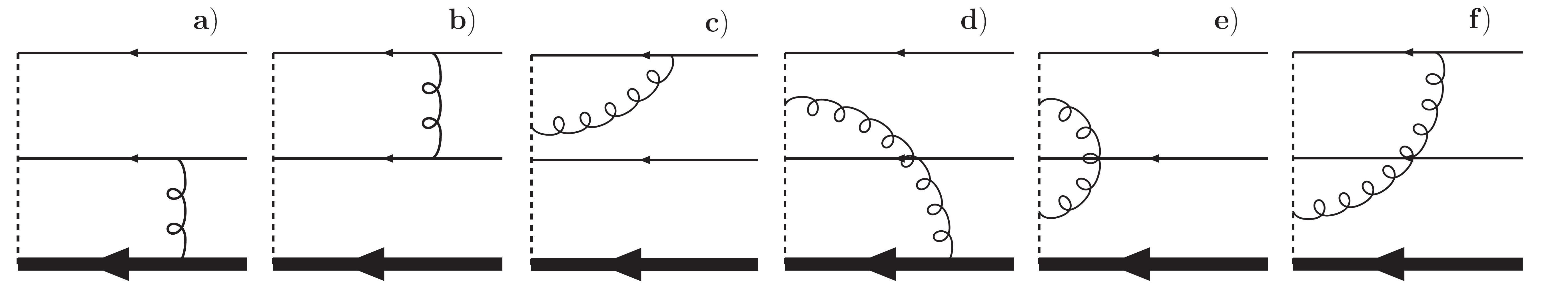
Figure 3: Types of diagrams for the non-local vertex renormalization. Each of the diagrams a), c), d) and f) appears twice (one for each light quark). The thick and thin solid lines correspond to the heavy and light quarks, respectively, and the dashed line represents the gauge link (Wilson line).

For the leading twist (neglecting masses) the diagrams give the same contribution for the $SU(3)_{\rm F}$ triplet and sextet (Fig. 1), where only for the transverse distribution amplitude diagram b) vanishes. The $SU(3)_{\rm F}$ triplet evolution equation has already been derived in Ball:2008fw .

At one-loop order the diagrams shown in Fig. 3 involve at the maximum two quarks in the loop. Hence, the derivation of the evolution kernels is almost identical to the meson case. The heavy-light contributions, involving the $b$-quark and one light quark, are similar to the heavy-light mesons Lange:2003ff and the light-light contributions are similar to the light-light mesons Ball:2003sc . The diagram a) is UV finite as it is found in Lange:2003ff . The diagram e) vanishes since the corresponding vertex is proportional to $n^{\mu}n^{\nu}$ and the gluon propagator is proportional to $g_{\mu\nu}$. The evolution equation for the leading twist reads Ball:2008fw :

$$\mu\,\frac{d}{d\mu}\,\psi^{n}(\omega_{1},\omega_{2};\mu)=-\frac{\alpha_{s}(\mu)}{2\pi}\left(1+\frac{1}{N_{c}}\right)\left[\int\limits_{0}^{\infty}dk_{1+}\,\gamma^{\rm LN}(\omega_{1},k_{1+};\mu)\,\psi^{n}(k_{1+},\omega_{2};\mu)\right.$$

$$\hskip 28.45274pt\left.+\int\limits_{0}^{\infty}dk_{2+}\,\gamma^{\rm LN}(\omega_{2},k_{2+};\mu)\,\psi^{n}(\omega_{1},k_{2+};\mu)-\int\limits_{0}^{1}dv\,V(u,v)\,\psi^{n}(v\omega,\bar{v}\omega;\mu)+\frac{3}{2}\,\psi^{n}(\omega_{1},\omega_{2};\mu)\right],$$ (38)

in which

$$\gamma^{\rm LN}(\omega,k_{+};\mu) = \ln\frac{\mu}{\omega}-\frac{5}{4}-\left[\frac{\omega}{k_{+}}\,\frac{\Theta(k_{+}-\omega)}{k_{+}-\omega}+\frac{\Theta(\omega-k_{+})}{\omega-k_{+}}\right]_{\oplus}$$ (39)

is taken from Lange:2003ff and $V(u,v)$ is the well-known Efremov-Radyushkin-Brodsky-Lepage kernel Efremov:1978rn ; Lepage:1979zb :

$$V(u,v) = \left[\frac{1-u}{1-v}\left(1+\frac{1}{u-v}\right)\Theta(u-v)+\frac{u}{v}\left(1+\frac{1}{v-u}\right)\Theta(v-u)\right]_{+},$$ (40)

For transverse leading-twist LCDA $\psi_{\perp}^{n}$ diagram b) vanishes and one needs to replace

$$V(u,v) \to V(u,v)-\left[\frac{1-u}{1-v}\,\Theta(u-v)+\frac{u}{v}\,\Theta(v-u)\right]_{+},$$ (41)

while the rest stays unchanged. This effect on the evolution is negligible. The “$\oplus$” and “$+$” subtractions are defined as follows:

$$\int\limits_{0}^{\infty}dk_{+}\left[\gamma(\omega,k_{+})\right]_{\oplus}f(k_{+})=\int\limits_{0}^{\infty}dk_{+}\gamma(\omega,k_{+})\left[f(k_{+})-f(\omega)\right],$$ (42)

$$\left[V(u,v)\right]_{+}=V(u,v)-\delta(u-v)\int\limits_{0}^{1}dt\,V(t,v).$$ (43)

For small evolution steps, $\ln(\mu/\mu_{0})\lesssim 1$, the differentiation with respect to $\mu$ in Eq. (38) is given by the linear approximation:

$$\mu\,\frac{d}{d\mu}\,\psi^{n}(\omega_{1},\omega_{2};\mu)\approx\frac{\psi^{n}(\omega_{1},\omega_{2};\mu)-\psi^{n}(\omega_{1},\omega_{2};\mu_{0})}{\ln(\mu/\mu_{0})},$$ (44)

and the evolution of the distribution amplitudes can be calculated easily by substituting the initial condition $\psi^{n}(\omega_{1},\omega_{2};\mu_{0})$ in the integrand in (38). In the following we give the parallel LCDAs as example. As will be shown, the effect of the renormalization is within the errors obtained from the variation of $A$ characterizing two different structures in the local interpolating currents.

6 QCD Sum Rules

Following the standard procedure of QCD sum rules Shifman:1978bx ; Shifman:1978by , we calculate the matrix elements defined in (24) and (25) by approximating the baryonic state $\left|H_{b}^{j=1}\right\rangle$ by the local current defined in (16), i. e., $\left|H_{b}^{j=1}(x)\right\rangle\approx J(x)\,\left|0\right\rangle$. The corresponding correlation function is defined by the matrix element $\Pi_{\Gamma\Gamma^{\prime}\gamma\gamma^{\prime}}(t_{1},t_{2},x)=i\left\langle 0\right|{\rm T}\left\{O_{\Gamma\gamma}(t_{1},t_{2})\overline{J}_{\Gamma^{\prime}\gamma^{\prime}}(x)\right\}\left|0\right\rangle$, in which $O_{\Gamma\gamma}(t_{1},t_{2})$ can be any non-local operator defined in Eqs. (24) and (25). The coefficient functions describe the propagation of the quarks inside the baryon from point $x$ to the light-cone started from the point $0$, which is parametrized by the light quark positions $t_{i}$, presented in Fig. 4. The procedure of constructing the QCD sum rules is well-known and results in the following general form:

$$\frac{1}{3}f_{k}\left(Af^{(1)}_{H_{b}^{j=1}}+Bf^{(2)}_{H_{b}^{j=1}}\right)\widetilde{\psi}^{\rm SR}_{k}(t_{1},t_{2})\,{\rm e}^{-\bar{\Lambda}/\tau}={\cal B}[\Pi_{k}](t_{1},t_{2};\tau,s_{0}),$$ (45)

where $f_{k}=f^{(1)}_{H_{b}^{j=1}}$ for the even twists and $f_{k}=f^{(2)}_{H_{b}^{j=1}}$ for the twist-3 parallel distribution amplitudes (and swapped according to (25) for the transverse twist). The effective baryon mass is introduced as the difference $\bar{\Lambda}=m_{H_{b}^{j=1}}-m_{b}$, $\tau$ is the Borel parameter, and $s_{0}$ is the continuum threshold. The r.h.s. in Eq. (45) is the Borel-transformed continuum-subtracted invariant function determined through the correlation function $\Pi_{k}(t_{1},t_{2};\tau,s_{0})$.

The Fourier transform of the correlation function is then given by

$$\Pi_{\Gamma\Gamma^{\prime}\gamma\gamma^{\prime}}(\omega_{1},\omega_{2};E)=\int\limits_{-\infty}^{\infty}\frac{dt_{1}}{2\pi}\,e^{i\omega_{1}t_{1}}\int\limits_{-\infty}^{\infty}\frac{dt_{2}}{2\pi}\,e^{i\omega_{2}t_{2}}\int d^{4}x\,e^{-iEv.x}\left\langle 0\right|O_{\Gamma\gamma}(t_{1},t_{2})\overline{J}_{\Gamma^{\prime}\gamma^{\prime}}(x)\left|0\right\rangle.$$ (46)

Inserting and contracting the quark fields and performing the Fourier transformations yields

$$\Pi_{\Gamma\Gamma^{\prime}}(\omega,u;E)_{\gamma\gamma^{\prime}}=-6i\int d^{4}x\,e^{-iEv.x}\,\left[\tilde{S}_{m=\infty}\right]_{\gamma\gamma^{\prime}}(x)\textnormal{Tr}\left[{\Gamma\tilde{S}_{q_{2}}(\bar{u}\omega,t)\Gamma^{\prime}\tilde{S}_{q_{1}}^{T}(u\omega,t)}\right].$$ (47)

The propagators $\tilde{S}_{q}$, discussed later, are not free but describe the dynamical evolution of the valence quarks within the low-energetic QCD background of the baryon by including condensate contributions.

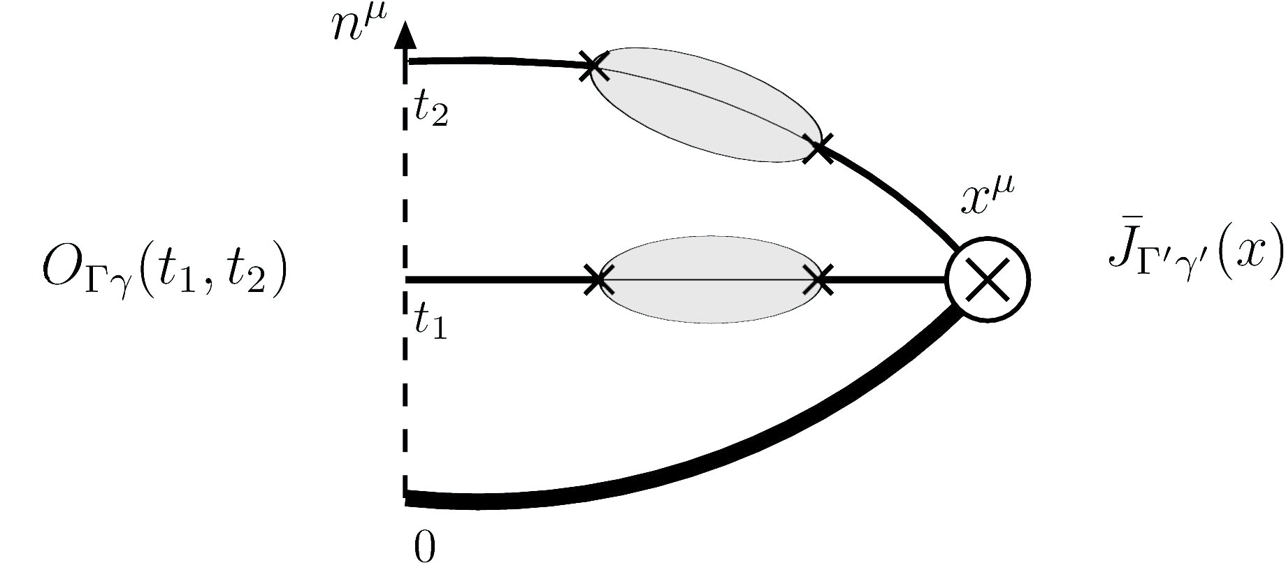
Figure 4: The correlation function in the QCD background. The light quarks move from the point $x$ in the QCD background (shaded regions) to the light-like direction $n^{\mu}$ (dashed line). The $b$-quark is indicated by the thick black line.

The heavy quark spin structure can be seen directly and is given by $P_{+}$, see Eq. (1). The light quark polarizations are given implicitly inside the trace by the $\Gamma$ and $\Gamma^{\prime}$ structures. The correlation functions must be proportional to the Lorentz structure given by the spin sum (1). The currents are then automatically projected on the proper polarization, such that

$$\Pi_{\Gamma_{\perp\mu}\Gamma^{\prime}_{\perp\nu}\gamma\gamma^{\prime}}(\omega,u;E) =\Pi_{\perp}(\omega,u;E)\left(-g_{\mu\nu}+v_{\mu}v_{\nu}+\varepsilon_{\parallel\mu}\varepsilon_{\parallel\nu}/\varepsilon_{\parallel}^{2}\right)\left[P_{+}\right]_{\gamma\gamma^{\prime}},$$

$$\Pi_{\Gamma_{\parallel\mu}\Gamma^{\prime}_{\parallel\nu}\gamma\gamma^{\prime}}(\omega,u;E) =-\Pi_{\parallel}(\omega,u;E)\left(\varepsilon_{\parallel\mu}\varepsilon_{\parallel\nu}/\varepsilon_{\parallel}^{2}\right)\left[P_{+}\right]_{\gamma\gamma^{\prime}},$$ (48)

which defines the scalar functions $\Pi_{\perp}(\omega,u;E)$ and $\Pi_{\parallel}(\omega,u;E)$. They are identical for the parallel and transverse polarizations up to different contributions of the local interpolating currents, which gives

$$\Pi_{\perp}(\omega,u;E)_{A,B}=\Pi_{\parallel}(\omega,u;E)_{B,A}.$$ (49)

Since the LCDAs are given for the central value $A=B=1/2$, the distribution functions $\psi(\omega,u:\mu)$ are the same for the transverse and parallel polarizations. The dependence of the correlation functions on $A$ and $B$ is due to our choice of the set of linear independent operators for the non-local currents in (24) and (25). Rewriting the parallel currents by introducing a different basis, for example $\gamma_{\parallel}^{\mu}$, would change the above described symmetry in $A$ and $B$.

The correlation functions are evaluated in the following by using configuration space techniques, instead of working in the more common momentum space. The reason is that the leading order sunrise-diagrams become very simple in the coordinate space. Sunrise diagrams are certain types of $1\to 1$ multi-loop self energy diagrams. (For a review about the evaluation of diagrams of the sunrise type in coordinate space see Groote:2005ay ). The non-local diagrams, which are necessary for the calculation of the LCDAs, differ in principle from the sunrise type because they do not involve two local interpolating currents, instead they are ripped open along a light-like line at the left side of the diagram pictured in Fig. 4. Hence, a more appropriate term would be lacerated sunrise diagram. But despite the difference, configuration space techniques work also well for this kind of diagrams (as shown below).

In the following we shortly introduce the different propagators of light and heavy quarks in the configuration space which are needed for the calculation of the correlation functions. In the heavy quark limit the Fourier transform of the heavy quark propagator has the very simple form of a classical point-like particle with a non-relativistic on-shell Dirac structure:

$$\tilde{S}_{m=\infty}(x) =\frac{1+\not{v}}{2}\int dt\,\delta^{4}(x-vt).$$ (50)

To take the effects of the QCD background for the propagators of the light quark fields into account, the method of non-local condensates Mikhailov:1986be ; Mikhailov:1991pt is used. The propagator is then given by a sum of the free propagator $S_{q}(x)$ and the universal non-perturbative part $\mathcal{C}_{q}(x)$:

$$\begin{array}[]{lllll}\raisebox{-1.0pt}[-20.0pt][-20.0pt]{$\scriptstyle{\tilde{S}_{q}(x)}$}&&\raisebox{-1.0pt}[-20.0pt][-20.0pt]{$\scriptstyle{S_{q}(x)}$}&&\raisebox{-1.0pt}[-20.0pt][-20.0pt]{$\scriptstyle{\mathcal{C}_{q}(x)}$}\\ \raisebox{-5.0pt}{\includegraphics[width=94.09265pt]{propcon0.pdf}}&=&\raisebox{0.0pt}{\includegraphics[width=94.09265pt]{propcon1.pdf}}&+&\raisebox{-5.0pt}{\includegraphics[width=94.09265pt]{propcon2.pdf}}\end{array}$$ (51)

with

$$S_{q}(x)=\frac{i}{2\pi^{2}}\,\frac{\not{x}}{x^{4}}-\frac{m_{q}}{4\pi^{2}x^{2}},\enspace\enspace\enspace\enspace\enspace\enspace\mathcal{C}_{q}(x)=\frac{1}{12}<\bar{q}(x)q(0)>,$$ (52)

in which color and spin indices are omitted since the color structure is simply given by the Kronecker delta. For the non-local condensate we adopt the model proposed in Braun:1994jq ; Braun:2003wx :

$$<\bar{q}(x)q(0)>=<\bar{q}q>\int\limits_{0}^{\infty}d\nu e^{\nu x^{2}/4}f(\nu),$$ (53)

$$f(\nu)=\frac{\lambda^{a-2}}{\Gamma(a-2)}\,\nu^{1-a}\,e^{-\lambda/\nu},\qquad a-3=\frac{4\lambda}{m_{0}^{2}},$$

in which $<\bar{q}q>$ is the local condensate, $m_{0}^{2}$ is the ratio of the mixed quark-gluon and quark condensate, and $\lambda$ is the correlation length. For completeness we also give the Fourier transformed operators ($t_{i}\to\omega_{i}$, $\omega_{1}=u\omega$, $\omega_{2}=\bar{u}\omega$), which are used in Eq. (47):

$$S_{q}(u\omega,t) =-ie^{i\,\frac{u\omega t}{2v_{+}}}\,\frac{2m_{q}tv_{+}+u\omega tv_{+}\not{\bar{n}}+2i\not{n}}{8\pi t^{2}v_{+}^{2}},$$

$$\mathcal{C}_{q}(u\omega,t) =\frac{\pi<\bar{q}q>}{3tv_{+}}\,e^{i\,\frac{tu\omega}{2v_{+}}}\,f\left(\frac{2u\omega i}{tv_{+}}\right).$$ (54)

The non-local condensate can be interpreted as the contribution of the quark, which descends to the non-perturbative sea of particles populating the QCD background, at one point and reemerges at a different point. It is still a question to what extent this sea is universal to the collective of all hadrons. Moreover, little is known about the shape of these functions, and different models, such as Bakulev:2002hk , have been proposed in the literature to describe this non-perturbative behavior.

Inserting the propagators in the QCD background, Eq. (47) reads diagrammatically

$$\Pi(\omega,u;E)=\raisebox{-14.0pt}{\includegraphics[width=47.04991pt]{SRschem1.pdf}}+\raisebox{-14.0pt}{\includegraphics[width=47.04991pt]{SRschem2.pdf}}+\raisebox{-14.0pt}{\includegraphics[width=47.04991pt]{SRschem3.pdf}}+\raisebox{-14.0pt}{\includegraphics[width=47.04991pt]{SRschem4.pdf}},$$ (55)

in which the thin lines correspond to the light quarks and the thick line corresponds to the $b$-quark. There is no $b$-quark condensate term, since it is suppressed by $1/m_{b}$, and hence it vanishes in the heavy quark limit.

The Borel transform can easily be applied together with the Fourier transform, since for a function $f(t)$

$$\mathds{B}\left[\int e^{iEt}\,f(t)\,dt\right]_{E\to\tau}=i\,f\left(\frac{i}{\tau}\right)$$ (56)

holds. As known, the Borel transform handles the UV divergences automatically, making renormalization rather easy. As a short reminder, the renormalization condition is applied by adding a certain polynomial in $E$ to remove the UV divergent terms, which vanishes due to the derivative of arbitrary order in $E$ in the Borel transform.

The momentum cutoff is applied by cutting off the upper spectrum of the Laplace transform $L^{-1}$ (mapping to the spectral density) of the perturbative contributions, i. e.,

$$f(\tau)\stackrel{{\scriptstyle L^{-1}}}{{\longrightarrow}}\int\limits_{s_{\rm min}}^{\infty}\,e^{-s/\tau}\,\tilde{f}(s)\,ds\stackrel{{\scriptstyle\textnormal{cutoff}}}{{\longrightarrow}}\int\limits_{s_{\rm min}}^{s_{0}}\,e^{-s/\tau}\,\tilde{f}(s)\,ds,$$ (57)

using

$$e^{-\Omega/\tau}\,\tau^{a}=\frac{1}{\Gamma(a)}\int\limits_{\Omega}^{\infty}ds\,e^{-s/\tau}\,(s-\Omega)^{a-1}.$$ (58)

One has to be careful, however, what one calls perturbative since there might be mixed perturbative and condensate contributions. Mixed contributions originate from diagrams in which one light quark is described by the low-energy condensate and the other light quark is described by the high-energy perturbative propagator. We adopted the procedure of Ball:2008fw and call the distribution perturbative when at least one perturbative term is present. This procedure leads to incomplete $\Gamma$-functions. For book keeping, we introduce the function

$$E_{a}(x)\equiv\frac{1}{\Gamma(a+1)}\int_{0}^{x}dt\,t^{a}{\rm e}^{-t}=1-\frac{\Gamma(a+1,x)}{\Gamma(a+1)},$$ (59)

in which $\Gamma(a+1,x)=\int_{x}^{\infty}dt\,t^{a}{\rm e}^{-t}$ is the incomplete $\Gamma$-function. The application of the quark-hadron duality thus results in $e^{-\Omega/\tau}\,\tau^{a}\to e^{-\Omega/\tau}\,\tau^{a}\,E_{a-1}(s_{0}-\Omega)$. For $a=N\in\mathds{N}$, this function is reduced to the well-known form

$$E_{N}(x)=1-{\rm e}^{-x}\sum_{n=0}^{N}\frac{x^{n}}{n!}.$$ (60)

In numerical estimates, it is also helpful to use the relation

$$E_{a}(x)=E_{a+1}(x)+\frac{x^{a+1}\,{\rm e}^{-x}}{\Gamma(a+2)},$$ (61)

obtained from (59) after integration by parts, connecting the negative value of the parameter $a$ in $E_{a}(x)$ with a corresponding positive one.

Inserting the propagators (52) and (54) in Eq. (47) and performing the Borel and Fourier transforms, the sum rules defined in (45) are obtained in a straightforward way. We summarize our sum rule results where the leading-twist transverse formula is given as

$$\frac{1}{3}f^{(2)}_{H_{b}^{j=1}}\left(Af^{(1)}_{H_{b}^{j=1}}+Bf^{(2)}_{H_{b}^{j=1}}\right)\tilde{\psi}_{\perp}^{n}(\omega,u)\,{\rm e}^{-\bar{\Lambda}/\tau}=$$ (62)

$$\quad\hphantom{=}\frac{3\tau^{4}}{2\pi^{4}}\,\left[B\hat{\omega}^{2}\,u\bar{u}+A\,\hat{\omega}\left(\hat{m}_{2}u+\hat{m}_{1}\bar{u}\right)\right]E_{1}(2\hat{s}_{\omega}){\rm e}^{-\hat{\omega}}$$

$$\quad-\frac{\langle\bar{q}_{1}q_{1}\rangle\tau^{3}}{\pi^{2}}\,\left[A\hat{\omega}\bar{u}+B\hat{m}_{2}\right]f(2\tau\omega u)\,E_{2-a}(2\hat{s}_{\kappa})\,{\rm e}^{-\hat{\omega}}$$

$$\quad-\frac{\langle\bar{q}_{2}q_{2}\rangle\tau^{3}}{\pi^{2}}\,\left[A\hat{\omega}u+B\hat{m}_{1}\right]f(2\tau\omega\bar{u})\,E_{2-a}(2\hat{s}_{\bar{\kappa}})\,{\rm e}^{-\hat{\omega}}$$

$$\quad+\frac{2B}{3}\,\langle\bar{q}_{1}q_{1}\rangle\,\langle\bar{q}_{2}q_{2}\rangle\,\tau^{2}\,f(2\tau\omega u)\,f(2\tau\omega\bar{u})\,E_{3-2a}(2\hat{s}_{\kappa\bar{\kappa}})\,{\rm e}^{-\hat{\omega}},$$

in which $s_{\omega}=s_{0}-\omega/2$, $\hat{m}=m/(2\tau)$, $\hat{\omega}=\omega/(2\tau)$, $\hat{s}_{\omega}=s_{\omega}/(2\tau)$, $\hat{s}_{\kappa}=\hat{s}_{\omega}-\kappa/2$, $\hat{s}_{\bar{\kappa}}=\hat{s}_{\omega}-\bar{\kappa}/2$, $\hat{s}_{\kappa\bar{\kappa}}=\hat{s}_{\omega}-\kappa/2-\bar{\kappa}/2$, and the short-hand notations

$$\kappa=\frac{\lambda}{2u\omega\tau},\qquad\bar{\kappa}=\frac{\lambda}{2\bar{u}\omega\tau}$$ (63)

are used. For the twist-3 and twist-4 LCDAs, the results can be derived analogously:

$$\frac{1}{3}f^{(1)}_{H_{b}^{j=1}}\left(Af^{(1)}_{H_{b}^{j=1}}+Bf^{(2)}_{H_{b}^{j=1}}\right)\tilde{\psi}_{\perp}^{\mathds{1}}(\omega,u)\,{\rm e}^{-\bar{\Lambda}/\tau}$$ (64)

$$\quad=\frac{3\tau^{4}}{4\pi^{4}}\left\{\left[A\hat{\omega}+B\,(\hat{m}_{1}+\hat{m}_{2})\right]E_{2}(2\hat{s}_{\omega})+B\hat{\omega}\,(\hat{m}_{2}u+\hat{m}_{1}\bar{u})\,E_{1}(2\hat{s}_{\omega})\right\}{\rm e}^{-\hat{\omega}}$$

$$\quad-\frac{\langle\bar{q}_{1}q_{1}\rangle\tau^{3}}{2\pi^{2}}\left[B\,E_{3-a}(2\hat{s}_{\kappa})+\left(B\hat{\omega}\bar{u}+2A\hat{m}_{2}\right)E_{2-a}(2\hat{s}_{\kappa})\right]f(2\tau\omega u)\,{\rm e}^{-\hat{\omega}}$$

$$\quad-\frac{\langle\bar{q}_{2}q_{2}\rangle\tau^{3}}{2\pi^{2}}\left[B\,E_{3-a}(2\hat{s}_{\bar{\kappa}})+\left(B\hat{\omega}u+2A\hat{m}_{1}\right)E_{2-a}(2\hat{s}_{\bar{\kappa}})\right]f(2\tau\omega\bar{u})\,{\rm e}^{-\hat{\omega}}$$

$$\quad+\frac{2A}{3}\,\langle\bar{q}_{1}q_{1}\rangle\,\langle\bar{q}_{2}q_{2}\rangle\,\tau^{2}\,f(2\tau\omega u)\,f(2\tau\omega\bar{u})\,E_{3-2a}(2\hat{s}_{\kappa\bar{\kappa}})\,{\rm e}^{-\hat{\omega}},$$

$$\frac{1}{3}f^{(1)}_{H_{b}^{j=1}}\left(Af^{(1)}_{H_{b}^{j=1}}+Bf^{(2)}_{H_{b}^{j=1}}\right)\tilde{\psi}_{\perp}^{n\bar{n}}(\omega,u)\,{\rm e}^{-\bar{\Lambda}/\tau}$$ (65)

$$\quad=\frac{3\tau^{4}}{4\pi^{4}}\left\{\left[A\hat{\omega}\,(u-\bar{u})+B\,(\hat{m}_{1}-\hat{m}_{2})\right]E_{2}(2\hat{s}_{\omega})+B\hat{\omega}\,(\hat{m}_{2}u-\hat{m}_{1}\bar{u})E_{1}(2\hat{s}_{\omega})\right\}{\rm e}^{-\hat{\omega}}$$

$$\quad-\frac{B\langle\bar{q}_{1}q_{1}\rangle\tau^{3}}{2\pi^{2}}\,\left[E_{3-a}(2\hat{s}_{\kappa})-\hat{\omega}\bar{u}\,E_{2-a}(2\hat{s}_{\kappa})\right]f(2\tau\omega u)\,{\rm e}^{-\hat{\omega}}$$

$$\quad+\frac{B\langle\bar{q}_{2}q_{2}\rangle\tau^{3}}{2\pi^{2}}\,\left[E_{3-a}(2\hat{s}_{\bar{\kappa}})-\hat{\omega}u\,E_{2-a}(2\hat{s}_{\bar{\kappa}})\right]f(2\tau\omega\bar{u})\,{\rm e}^{-\hat{\omega}},$$

$$\frac{1}{3}f^{(2)}_{H_{b}^{j=1}}\left(Af^{(1)}_{H_{b}^{j=1}}+Bf^{(2)}_{H_{b}^{j=1}}\right)\tilde{\psi}_{\perp}^{\bar{n}}(\omega,u)\,{\rm e}^{-\bar{\Lambda}/\tau}$$ (66)

$$\quad=\frac{3\tau^{4}}{2\pi^{4}}\left[B\,E_{3}(2\hat{s}_{\omega})+A\left(\hat{m}_{1}+\hat{m}_{2}\right)E_{2}(2\hat{s}_{\omega})\right]{\rm e}^{-\hat{\omega}}$$

$$\quad-\frac{\langle\bar{q}_{1}q_{1}\rangle\tau^{3}}{\pi^{2}}\,\left[A\,E_{3-a}(2\hat{s}_{\kappa})+B\hat{m}_{2}\,E_{2-a}(2\hat{s}_{\kappa})\right]f(2\tau\omega u)\,{\rm e}^{-\hat{\omega}}$$

$$\quad-\frac{\langle\bar{q}_{2}q_{2}\rangle\tau^{3}}{\pi^{2}}\,\left[A\,E_{3-a}(2\hat{s}_{\bar{\kappa}})+B\hat{m}_{1}\,E_{2-a}(2\hat{s}_{\bar{\kappa}})\right]f(2\tau\omega\bar{u})\,{\rm e}^{-\hat{\omega}}$$

$$\quad+\frac{2B}{3}\,\langle\bar{q}_{1}q_{1}\rangle\,\langle\bar{q}_{2}q_{2}\rangle\,\tau^{2}\,f(2\tau\omega u)\,f(2\tau\omega\bar{u})\,E_{3-2a}(2\hat{s}_{\kappa\bar{\kappa}})\,{\rm e}^{-\hat{\omega}}.$$

The result for the parallel counterpart can be obtained by the replacement $A\leftrightarrow B$.

The QCD sum rules given in (62) can not be used in calculations directly. The main reason for this is that the sum rules are built from a patchwork of different contributions, the perturbative and condensate parts. They show neither smooth behavior, nor necessarily the correct asymptotic behavior, i. e., the asymptotic behavior of the perturbative contribution. As a consequence, one has to propose model functions which are then constrained by the sum rules. The LCDA models are discussed below in Sec. 7.

7 LCDA Models

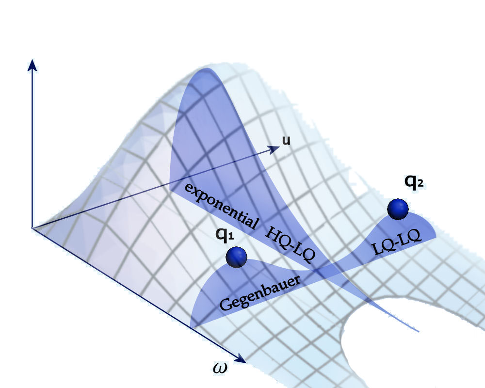
Figure 5: Model functions for the $b$-baryon LCDAs, composed of the exponential part for the heavy-light interaction and the Gegenbauer polynomials for the light-light interaction.

Table 3: Moments for the LCDA model functions in terms of their parameters.

twist	$\langle 1\rangle$	$\langle\omega^{-1}\rangle$	$\langle C^{3/2}_{1}\rangle$	$\langle\omega^{-1}C^{3/2}_{1}\rangle$	$\langle C^{3/2}_{2}\rangle$	$\langle\omega^{-1}C^{3/2}_{2}\rangle$
$2$	$a_{0}$	$a_{0}/3\varepsilon_{0}$	$3a_{1}/5$	$a_{1}/5\varepsilon_{1}$	$3a_{2}/7$	$a_{2}/7\varepsilon_{2}$
twist	$\langle 1\rangle$	$\langle\omega^{-1}\rangle$	$\langle C^{1/2}_{1}\rangle$	$\langle\omega^{-1}C^{1/2}_{1}\rangle$	$\langle C^{1/2}_{2}\rangle$	$\langle\omega^{-1}C^{1/2}_{2}\rangle$
$3$	$a_{0}$	$a_{0}/2\varepsilon_{0}$	$a_{1}$	$a_{1}/2\varepsilon_{1}$	$a_{2}$	$a_{2}/2\varepsilon_{2}$
$4$	$a_{0}$	$a_{0}/\varepsilon_{0}$	$a_{1}$	$a_{1}/\varepsilon_{1}$	$a_{2}$	$a_{2}/\varepsilon_{2}$

In the parametrization, in which the baryon is described by the total energy of the light quark system $\omega$ and the momentum fractions $u$ and $\bar{u}$, the following arguments become manifest. The dynamics of the heavy-light baryon part, i. e., the dynamics of the heavy quark and the light diquark, is described with the same formalism which has worked well for the heavy-light meson dynamics. The dynamics of the light quarks in the diquark is then described in the same way as the light-light mesons. This ansatz is consistent with the equations of motion for the light quarks Ball:1998sk . In conclusion we choose the multiplicative ansatz from Ball:2008fw . In this approach the Gegenbauer polynomials $C^{\lambda}_{n}(x)$ Bateman-vII take the light quarks into account and an exponential factor characterizes the dynamics of the heavy-light system, as shown in Fig. 5. It is more convenient to choose $C^{3/2}_{n}(x)$ Gegenbauer polynomials for twist-2 but $C^{1/2}_{n}(x)$ for the other twist functions similar to the expansion of the vector mesons Ball:1998sk . The first three polynomials are sufficient to account for the precision in this work. They are defined as follows:

$$C^{\lambda}_{0}(x)=1,\enspace\enspace\enspace C^{\lambda}_{1}(x)=2\lambda x,\enspace\enspace\enspace C^{\lambda}_{2}(x)=2\lambda\left(1+\lambda\right)x^{2}-\lambda.$$ (67)

To obtain the model fit, we calculate the momentum fraction integrals (the moments) which are defined for an arbitrary function $f(\omega,u)$ as:

$$\langle f(\omega,u)\rangle^{H_{b}^{j}}_{k}\equiv\int_{0}^{2s_{0}}\omega d\omega\int_{0}^{1}du\,f(\omega,u)\,\tilde{\psi}^{\rm SR}_{k}(\omega,u).$$ (68)

The model functions for the LCDAs of different twists are:

$$\tilde{\psi}_{2}(\omega,u) = \omega^{2}u(1-u)\,\sum_{n=0}^{2}\frac{a_{n}}{{\epsilon_{n}}^{4}}\,\frac{C^{3/2}_{n}(2u-1)}{|C^{3/2}_{n}|^{2}}\,{\rm e}^{-\omega/\epsilon_{n}},$$ (69)

$$\tilde{\psi}_{3}(\omega,u) = \frac{\omega}{2}\,\sum_{n=0}^{2}\frac{a_{n}}{{\epsilon_{n}}^{3}}\,\frac{C^{1/2}_{n}(2u-1)}{|C^{1/2}_{n}|^{2}}\,{\rm e}^{-\omega/\epsilon_{n}},$$ (70)

$$\tilde{\psi}_{4}(\omega,u) = \sum_{n=0}^{2}\frac{a_{n}}{{\epsilon_{n}}^{2}}\,\frac{C^{1/2}_{n}(2u-1)}{|C^{1/2}_{n}|^{2}}\,{\rm e}^{-\omega/\epsilon_{n}},$$ (71)

in which the twist is indicated by the subscript numbers and

$$\left|C^{\lambda}_{n}\right|^{2}=\int_{0}^{1}du\left[C^{\lambda}_{n}(2u-1)\right]^{2},$$ (72)

with $\big{|}C^{1/2}_{0}\big{|}^{2}=\big{|}C^{3/2}_{0}\big{|}^{2}=1$, $\big{|}C^{1/2}_{1}\big{|}^{2}=1/3$, $\big{|}C^{3/2}_{1}\big{|}^{2}=3$, $\big{|}C^{1/2}_{2}\big{|}^{2}=1/5$, and $\big{|}C^{3/2}_{2}\big{|}^{2}=6$. The prefactors in front of the sums in Eq. (69) — (71) ($\omega^{2}u(1-u)$, etc.) are determined by the corresponding perturbative part in order to give the correct asymptotic behavior (compare the $B$ term in the first line in Eq. (62)). The parameters $\epsilon_{i}$ are strictly positive to satisfy the asymptotic behavior. The moments of the functions (69) — (71) which are calculated with the use of (68) are listed in Tab. 3.

In the construction of the models for the LCDAs, we have truncated the Gegenbauer expansion at the second non-asymptotic term and have taken the limit $s_{0}\to\infty$ in the integral over $\omega$ which has negligible effect.

8 Results and Numerical Analysis

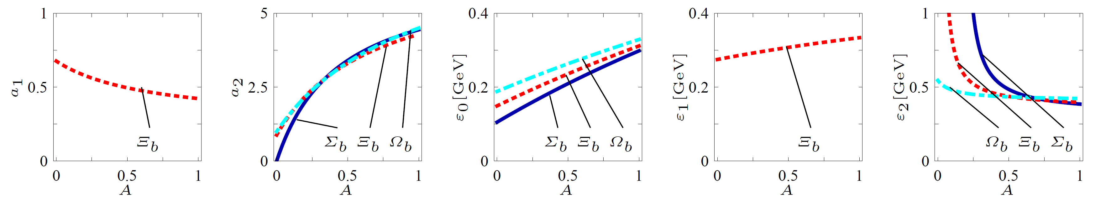
Figure 6: The dependence of the transverse twist-2 model parameters listed in Tab. 5 on the variation of the coefficient $A$ of the local interpolating currents (the parallel ones are obtained by the replacement $A\to 1-A$).

Table 4: Input values from Refs. Ball:2008fw ; Shifman:1978by ; Chetyrkin:2007vm ; Chernyak:1983ej . For $\bar{\Lambda}$ and $s_{0}$, see Tab. 1.

$m_{u,d}$	0			$\langle\bar{q}q\rangle$	$-242$ MeV3
$m_{s}$	$128$ MeV			$\langle\bar{s}s\rangle/\langle\bar{q}q\rangle$	$0.8$
$\lambda$	$0.16$ GeV2			$m_{0}^{2}=\langle\bar{q}D^{2}q\rangle/\langle\bar{q}q\rangle$	$0.8$ GeV2
$\tau$	$0.6$ GeV			$m_{s0}^{2}=\langle\bar{s}D^{2}s\rangle/\langle\bar{s}s\rangle$	$1.36$ GeV2

The moments of the functions defined in Eqs. (69) — (71) can be calculated using (68). To perform a numerical analysis, we discuss and specify the required input parameters which are summarized in Tab. 4. The values of the effective baryon masses $\bar{\Lambda}=m_{H_{b}^{j}}-m_{b}$ in the HQET for $m_{b}=4.8$ GeV are presented in Tab. 1 where experimental measurements Beringer:1900zz and theoretical predictions (based on the HQET Liu:2007fg and Lattice QCD Lewis:2008fu ) for the masses (in units of MeV) of the ground-state bottom baryons are also shown. A comparative analysis of predictions for the heavy-baryon masses can be found in Refs. Liu:2007fg ; Zhang:2008pm . The continuum threshold values $s_{0}$ (the last column in Tab. 1) used by us are in agreement with the ones from Liu:2007fg derived for the baryon-mass evaluated to order $1/m_{b}$ within the HQET. For the discussion of these parameters see Chetyrkin:2007vm and references therein. Note that the shape function $f(\nu)$ in the non-local quark condensate (53) is assumed to be flavor independent for all light quarks.

Table 5: Parameters for the model functions in Eqs. (69) — (71) for the transverse LCDAs (the parallel ones are obtained by the replacement $A\to 1-A$ and the $\Lambda_{b}$ and $\Xi_{b}$ currents correspond to the parallel $\Sigma_{b}$ and $\Xi^{\prime}_{b}$ ones, respectively). For twist-2 LCDAs, the parameter dependence on $A$ is plotted in Fig. 6. The twist notations 3a and 3s correspond to the LCDAs $\psi^{n\bar{n}}$ and $\psi^{\mathds{1}}$, respectively.

$\Sigma_{b}$	twist	$a_{0}$	$a_{1}$	$a_{2}$	$\varepsilon_{0}$[GeV]	$\varepsilon_{1}$[GeV]	$\varepsilon_{2}$[GeV]
	$2$	$1$	$-$	$\frac{6.4A}{A+0.44}$	$\frac{1.4A+0.6}{A+5.7}$	$-$	$\frac{0.32A}{A-0.17}$
	$3s$	$1$	$-$	$\frac{0.12A-0.08}{A-1.4}$	$\frac{0.56A-0.77}{A-2.6}$	$-$	$\frac{0.25A-0.16}{A+0.41}$
	$3a$	$-$	$1$	$-$	$-$	$\frac{0.35A-0.43}{A-1.2}$	$-$
	$4$	$1$	$-$	$\frac{-0.07A-0.05}{A+0.34}$	$\frac{0.65A+0.22}{A+1}$	$-$	$\frac{5.5A+3.8}{A+29}$
$\Xi_{b}^{\prime}$	twist	$a_{0}$	$a_{1}$	$a_{2}$	$\varepsilon_{0}$	$\varepsilon_{1}$	$\varepsilon_{2}$
	$2$	$1$	$\frac{0.25A+0.46}{A+0.68}$	$\frac{6.6A+0.6}{A+0.68}$	$\frac{1.4A+1}{A+6.7}$	$\frac{0.57A+1.1}{A+4}$	$\frac{0.36A+0.03}{A-0.02}$
	$3s$	$1$	$\frac{0.04A-0.14}{A-1.6}$	$\frac{0.12A-0.09}{A-1.6}$	$\frac{0.56A-0.91}{A-2.9}$	$\frac{-27A+92}{160}$	$\frac{0.3A-0.24}{A+0.54}$
	$3a$	$\frac{-0.16A+0.16}{A-1.3}$	$1$	$\frac{0.17A-0.17}{A-1.3}$	$\frac{0.11A-0.11}{A-1}$	$\frac{0.39A-0.49}{A-1.3}$	$\frac{0.33A-0.33}{A-1}$
	$4$	$1$	$\frac{0.03A+0.11}{A+0.16}$	$\frac{-0.1A-0.03}{A+0.61}$	$\frac{0.63A+0.38}{A+1.3}$	$\frac{-0.82A-3.1}{A-3.9}$	$\frac{1.2A+0.34}{A+4.1}$
$\Omega_{b}$	twist	$a_{0}$	$a_{1}$	$a_{2}$	$\varepsilon_{0}$	$\varepsilon_{1}$	$\varepsilon_{2}$
	$2$	$1$	$-$	$\frac{8A+1}{A+1}$	$\frac{1.3A+1.3}{A+6.9}$	$-$	$\frac{0.41A+0.06}{A+0.11}$
	$3s$	$1$	$-$	$\frac{0.17A-0.16}{A-2}$	$\frac{0.56A-1.1}{A-3.22}$	$-$	$\frac{0.44A-0.43}{A+0.27}$
	$3a$	$-$	$1$	$-$	$-$	$\frac{0.45A-0.63}{A-1.4}$	$-$
	$4$	$1$	$-$	$\frac{-0.10A-0.01}{A+1}$	$\frac{0.62A+0.62}{A+1.62}$	$-$	$\frac{0.87A+0.07}{A+2.53}$

The calculation is performed in the $b$-baryon rest frame with $v_{+}=1$ at an energy scale of $\mu=1$ GeV. The method of the non-local condensates which involves the parameters $\lambda$ and $m_{0}^{2}$ is not yet completely understood. Especially, since there is only one model parameter known, namely the ratio

$$m_{0}^{2} =\frac{\langle\bar{q}D^{2}q\rangle}{\langle\bar{q}q\rangle}$$ (73)

of the 5-dimensional and 3-dimensional local condensates. This parameter determines the center of the quark virtuality distribution in the QCD background, but is not sufficient to determine the shape of the quark distribution. To determine the form, also yet unknown dimension-7 local condensates are needed. We took the shape parameter $\lambda$ as the universal parameter which is not influenced by either the baryon or the mass of the propagating quark. For the strange quark, where

$$m_{s0}^{2}=\frac{\langle\bar{s}D^{2}s\rangle}{\langle\bar{s}s\rangle},$$ (74)

the situation is more difficult since even dimension-5 condensates are not yet clearly understood. The value $R$, which is defined by

$$R=\frac{\langle\bar{s}D^{2}s\rangle}{\langle\bar{q}D^{2}q\rangle},$$ (75)

varies from $R\approx 0.8$ Chernyak:1983ej ; Lee:1997ix which gives $m_{0}^{2}\approx m_{s0}^{2}$ to values around $R\approx 1.3$ Beneke:1992ba ; Dosch:2000ej ; Dosch:1988vv which gives

$$m_{s0}^{2}\approx 1.7\,m_{0}^{2},$$ (76)

which we took for our calculation since in this case the $SU(3)_{\rm F}$-breaking effects appear already in the lower $\omega$-spectrum. The influence of the choice of $R$ on our results is within the already large uncertainties due to the other parameters.

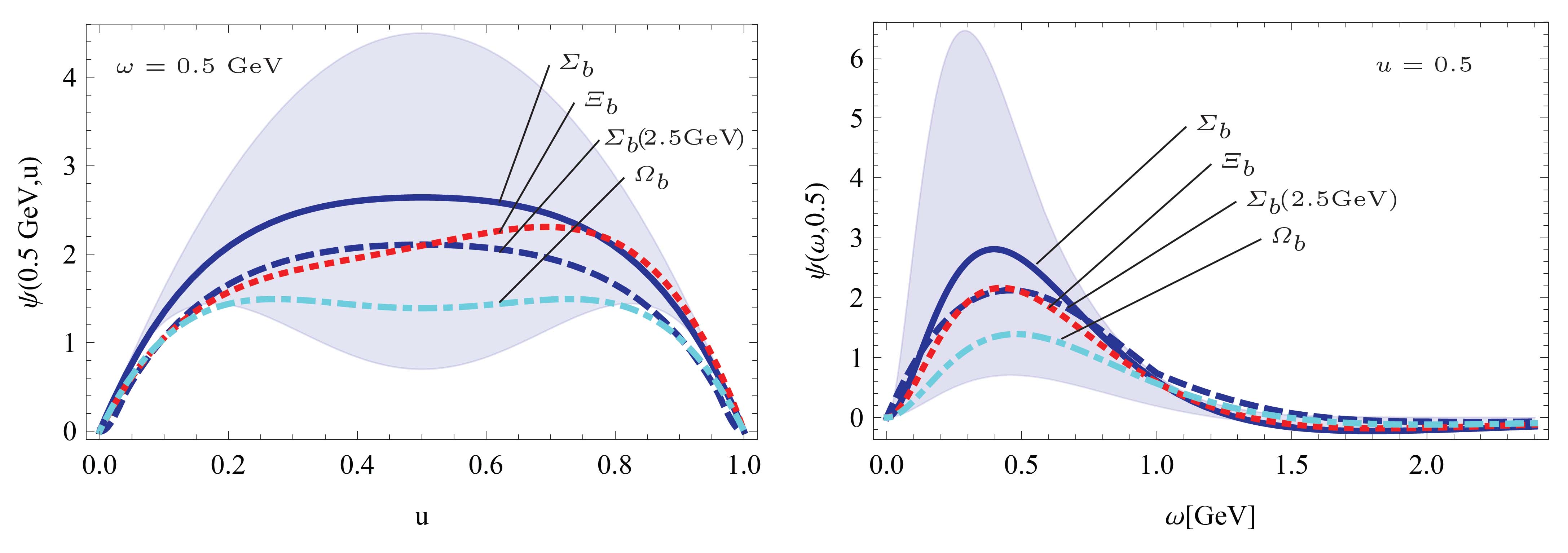
Figure 7: (Color online) The Twist 2 functions of $\Sigma_{b}$ (blue, solid), $\Xi_{b}$ (red, dashed) and $\Omega_{b}$ (cyan, dot-dashed) at the energy scale $\mu=1\;\textnormal{GeV}$ (blue, solid line) and the energy scale $\mu=2.5\;\textnormal{GeV}$ (blue, dashed line) including the most conservative error $A\in[0,1]$ for $\Sigma_{b}$ (blue, shaded region).

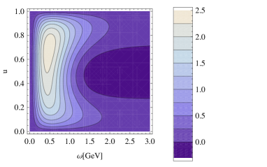
Figure 8: Model function $\psi(\omega,u)$ of the $b$-baryon $\Xi_{b}$. Shown are the twist 2 (upper left hand), symmetric twist 3 (upper right hand), antisymmetric twist 3 (lower left hand) and twist 4 (lower right hand) LCDAs. All entires are evaluated at the energy scale $\mu=1\;\textnormal{GeV}$.

With Tab. 3 the model parameters are extracted from the moments and collected in Tab. 5 in which the first moment is $1$ by definition according to (27), and the $\epsilon_{i}$ are required to be non-negative. The twist 2 model parameter dependence on $A$ is given in Fig. 6 as example. To give an overview over the tables of model parameters, we show the plots of the LCDAs in Fig 7 in the $\omega$ and $u$ distributions. The corresponding LCDAs for $\Xi_{b}$ ($\Xi^{\prime}_{b}$) in the ($\omega$, $u$) plane are shown in Fig. 8 as example.

9 Conclusions

As shown in Fig. 1 we are able to obtain the LCDAs for the entire ground-state multiplets of the bottom baryons with one heavy quark, thereby generalizing the work by Ball, Braun and Gardi Ball:2008fw . We accounted for the mass-breaking effects due to the strange-quark mass and calculated the evolution of the LCDAs with the use of the renormalization group equations, obtained from the one-loop renormalization of the non-local light-cone operators given in Eqs. (24) and (25). The resulting LCDAs are plotted in Figs. 7 and 8 in which the evolution from $\mu=1$ GeV to $\mu=2.5$ GeV and our error estimates are also shown. We find that the $SU(3)_{\rm F}$-breaking effects are of order 10 percent. The sources for the $SU(3)_{\rm F}$ breaking are the strange-quark mass, the Borel parameter $\tau$, the momentum cutoff $s_{0}$ and the non-local condensates. The latter ones are not well determined in the case of the strange quark. However, the mass-breaking effects appear in the lower part of the $\omega$-spectrum in the region of the constituent $s$-quark mass, as expected. Even though the $SU(3)_{\rm F}$-breaking effects appear to be quite large at some momenta, they are within the conservative errors for the massless case, as is the evolution to the energy scale $\mu=2.5$ GeV. The errors are obtained by varying the parameter $A$ in the full possible range $[0,1]$, which defines the linear superposition of the two local interpolating currents, given in Eq. (16). Reducing the variation of $A$ to the less conservative range $[0.3,0.7]$ results in a variation of the distribution amplitudes of roughly the same size as the evolution to $\mu=2.5$ GeV.

References

- (1) M. Artuso et al., Eur. Phys. J. C 57, 309 (2008) [arXiv:0801.1833 [hep-ph]].
- (2) W. Loinaz and R. Akhoury, Phys. Rev. D 53, 1416 (1996) [arXiv:hep-ph/9505378].
- (3) F. Hussain, J. G. Korner, M. Kramer and G. Thompson, Z. Phys. C 51, 321 (1991).
- (4) N. Isgur and M. B. Wise, Nucl. Phys. B 348 (1991) 276.
- (5) T. Mannel, W. Roberts and Z. Ryzak, Nucl. Phys. B 355, 38 (1991).
- (6) T. Mannel and S. Recksiegel, J. Phys. G24, 979 (1998) [J. Phys. G 24, 979 (1998)] [arXiv:hep-ph/9701399].
- (7) T. Feldmann and M. W. Y. Yip, Phys. Rev. D 85, 014035 (2012) [Erratum-ibid. D 86, 079901 (2012)] [arXiv:1111.1844 [hep-ph]].
- (8) T. Mannel and Y. M. Wang, JHEP 1112, 067 (2011) [arXiv:1111.1849 [hep-ph]].
- (9) G. Hiller and A. Kagan, Phys. Rev. D 65, 074038 (2002) [arXiv:hep-ph/0108074].
- (10) G. Hiller, M. Knecht, F. Legger and T. Schietinger, Phys. Lett. B 649, 152 (2007) [arXiv:hep-ph/0702191].
- (11) Z. T. Wei, H. W. Ke and X. Q. Li, Phys. Rev. D 80, 094016 (2009) [arXiv:0909.0100 [hep-ph]].
- (12) W. Wang, Phys. Lett. B 708, 119 (2012) [arXiv:1112.0237 [hep-ph]].
- (13) P. Ball, V. M. Braun and E. Gardi, Phys. Lett. B 665, 197 (2008) [arXiv:0804.2424 [hep-ph]].
- (14) A. Ali, C. Hambrock and A. Y. .Parkhomenko, Theor. Math. Phys. 170, 2 (2012) [Teor. Mat. Fiz. 170, 5 (2012)].
- (15) J. Beringer et al. [Particle Data Group], Phys. Rev. D 86, 010001 (2012).
- (16) X. Liu, H. X. Chen, Y. R. Liu, A. Hosaka and S. L. Zhu, Phys. Rev. D 77, 014031 (2008) [arXiv:0710.0123 [hep-ph]].
- (17) R. Lewis and R. M. Woloshyn, Phys. Rev. D 79, 014502 (2009) [arXiv:0806.4783 [hep-lat]].
- (18) A. F. Falk, Nucl. Phys. B 378, 79 (1992).
- (19) A. G. Grozin, Springer Tracts Mod. Phys. 201, 1 (2004).
- (20) A. G. Grozin and O. I. Yakovlev, Phys. Lett. B 285, 254 (1992) [arXiv:hep-ph/9908364].
- (21) S. Groote, J. G. Korner and O. I. Yakovlev, Phys. Rev. D 56, 3943 (1997) [arXiv:hep-ph/9705447].
- (22) S. Groote, J. G. Korner and O. I. Yakovlev, Phys. Rev. D 55, 3016 (1997) [arXiv:hep-ph/9609469].
- (23) A. G. Grozin and M. Neubert, Phys. Rev. D 55, 272 (1997) [arXiv:hep-ph/9607366].
- (24) P. Ball, V. M. Braun, Y. Koike and K. Tanaka, Nucl. Phys. B 529, 323 (1998) [arXiv:hep-ph/9802299].
- (25) E. Bagan, M. Chabab, H. G. Dosch and S. Narison, Phys. Lett. B 301, 243 (1993).
- (26) B. O. Lange and M. Neubert, Phys. Rev. Lett. 91, 102001 (2003) [arXiv:hep-ph/0303082].
- (27) P. Ball and M. Boglione, Phys. Rev. D 68, 094006 (2003) [arXiv:hep-ph/0307337].
- (28) A. V. Efremov and A. V. Radyushkin, Theor. Math. Phys. 42, 97 (1980) [Teor. Mat. Fiz. 42, 147 (1980)]; Phys. Lett. B 94, 245 (1980).
- (29) G. P. Lepage and S. J. Brodsky, Phys. Lett. B 87, 359 (1979); Phys. Rev. D 22, 2157 (1980).
- (30) M. A. Shifman, A. I. Vainshtein and V. I. Zakharov, Nucl. Phys. B 147, 385 (1979).
- (31) M. A. Shifman, A. I. Vainshtein and V. I. Zakharov, Nucl. Phys. B 147, 448 (1979).
- (32) S. Groote, J. G. Korner and A. A. Pivovarov, Annals Phys. 322, 2374 (2007) [arXiv:hep-ph/0506286].
- (33) S. V. Mikhailov and A. V. Radyushkin, JETP Lett. 43, 712 (1986) [Pisma Zh. Eksp. Teor. Fiz. 43, 551 (1986)].
- (34) S. V. Mikhailov and A. V. Radyushkin, Phys. Rev. D 45, 1754 (1992).
- (35) V. Braun, P. Gornicki and L. Mankiewicz, Phys. Rev. D 51, 6036 (1995) [arXiv:hep-ph/9410318].
- (36) V. M. Braun, D. Y. Ivanov and G. P. Korchemsky, Phys. Rev. D 69, 034014 (2004) [arXiv:hep-ph/0309330].
- (37) A. P. Bakulev and S. V. Mikhailov, Phys. Rev. D 65, 114511 (2002) [arXiv:hep-ph/0203046].
- (38) A. Erdélyi, W. Magnus, F. Oberhettinger, and F. G. Tricomi, Higher Transcendental Functions. Vol. II. Based on notes left by Harry Bateman. McGraw-Hill, New-York, 1954.
- (39) K. G. Chetyrkin, A. Khodjamirian and A. A. Pivovarov, Phys. Lett. B 661, 250 (2008) [arXiv:0712.2999 [hep-ph]].
- (40) V. L. Chernyak and A. R. Zhitnitsky, Phys. Rept. 112, 173 (1984).
- (41) J. R. Zhang and M. Q. Huang, Phys. Rev. D 78, 094015 (2008) [arXiv:0811.3266 [hep-ph]].
- (42) F. X. Lee, Phys. Rev. C 57, 322 (1998) [arXiv:hep-ph/9707332].
- (43) M. Beneke and H. G. Dosch, Phys. Lett. B 284, 116 (1992).
- (44) H. G. Dosch, M. Eidemuller, M. Jamin and E. Meggiolaro, JHEP 0007, 023 (2000) [arXiv:hep-ph/0004040].
- (45) H. G. Dosch, M. Jamin and S. Narison, Phys. Lett. B 220, 251 (1989).