We analyze the impact of effective axial-vector coupling of the gluon on spin polarization observables in $t\bar{t}$ pair production at the LHC. Working at leading order in QCD, we compute the $t\bar{t}$ spin-correlation and left-right spin asymmetry coefficients in the helicity basis in the laboratory frame as functions of the new physics scale $\Lambda$ associated with this coupling. We found that the $t\bar{t}$ invariant mass dependent asymmetries are more sensitive to the scale $\Lambda$ than the corresponding inclusive ones, in particular when suitable cuts selecting high $t\bar{t}$ invariant mass regions are imposed. In the context of this scenario, we show that the LHC has potential either to confirm or to rule out the Tevatron FB top asymmetry anomaly by analyzing the $t\bar{t}$ spin-correlation and left-right polarization asymmetries. On the other hand, stringent lower bound on the new physics scale $\Lambda$ can be set in this scenario if no significant deviations from the SM predictions for those observables will be measured.

1 Introduction

Top-quark physics is undoubtedly the best framework where to study polarized processes at the level of fundamental interactions [1]. Discovered at Tevatron in 1995 [2], [3] and copiously produced both at the Tevatron and the Large Hadron Collider (LHC) [4], the top-quark is the heaviest elementary fermion with the measured mass of $m_{t}=172.9\pm 0.6\pm 0.9$ GeV and decay width of $\Gamma_{t}=2.0^{+0.7}_{-0.6}$ GeV [5]. Since the top life-time is shorter than the characteristic hadronization time-scale $\sim 1/\Lambda_{\rm QCD}$, with $\Lambda_{\rm QCD}$ the characteristic QCD energy scale, this guarantees that it will always decay before hadronizing. Indeed, the top decay, which is dominated by the weak decay channel $t\to Wb$, is expected to occur before its spin is flipped by strong interactions. This ensures that top spin-polarization at production level will be fully transferred to its decay products. Then, the spin of the top-quark can be accessed by measuring the angular distributions of the final state decay products. The QCD corrections to the $t\bar{t}$ pair production at hadron colliders can be safely computed at high orders in perturbation theory [6, 7, 8, 9, 10, 11, 12, 13, 14, 15, 16, 17, 18, 19, 20], which allow us to determine the top-quark polarization with high accuracy.

An interesting observable that can be measured with high precision at hadron colliders is the spin-correlation in the $t\bar{t}$ pair production. This observable was analyzed in [21, 22, 23, 24, 25, 26, 27, 28, 29, 30, 31, 32] at the leading order (LO), and is now known at the next to leading order (NLO) [33, 34] in the strong coupling in QCD, while more recently the NLO weak corrections [35] have been included. The standard model (SM) predicts that spins of the top- and antitop-quarks are strongly correlated, which is just a consequence of the partonic $t\bar{t}$ production mechanisms at hadron colliders. The tree-level partonic processes, contributing to the $t\bar{t}$ production at the LO in QCD, are the quark-antiquark and gluon-gluon annihilation processes, namely $q\bar{q}\to t\bar{t}$ and $gg\to t\bar{t}$ respectively [1]. While at Tevatron the first mechanism dominates, the second one is the leading $t\bar{t}$ production mechanism at the LHC, contributing to almost 90% of the $pp\to t\bar{t}X$ total cross section. Therefore, at low $t\bar{t}$ invariant mass, the top- and antitop-quarks are mainly produced at the LHC experiments in the left-left and right-right helicity configurations, due to the spin-1 nature of gluons [36]. The different production mechanisms and collision energies in the Tevatron and the LHC make the measurements of $t\bar{t}$ spin correlations in those experiments complementary to each other. This observable is also a very sensitive probe of new physics scenarios that contribute to the partonic $t\bar{t}$ production mechanisms, whilst keeping the $t\bar{t}$ production cross section at hadron colliders within experimental and theoretical bounds [23, 37, 38, 39, 40, 41].

Both CDF [42] and D0 [43, 44, 45] Collaborations at Tevatron have performed measurements of the $t\bar{t}$ spin-correlation which, within experimental errors, are in agreement with the NLO SM predictions. In particular, D0 Collaboration has reported an evidence for the spin-correlation in $t\bar{t}$ with a significance of 3.1$\sigma$ [45]. From the LHC, the ATLAS [46] and CMS [47] Collaborations have recently analyzed the $t\bar{t}$ spin correlation by analyzing $\sqrt{s}=7$ TeV data corresponding to an integrated luminosity of about 2.1 ${\rm fb}^{-1}$ and 5 ${\rm fb}^{-1}$, respectively. ATLAS has excluded the hypothesis of zero spin-correlation with a significance of 5.1 $\sigma$ [46], while the CMS has only reported a 2.9 $\sigma$ evidence [47]. Within experimental errors both measurements are consistent with the NLO SM predictions [35].

However, despite the good agreement between the SM and data in the top-quark sector, the 3$\sigma$ excess in the $t\bar{t}$ charge or forward-backward (FB) asymmetry with respect to the SM predictions [48, 49, 50], observed at Tevatron by the CDF [51] and D0 [52] Collaborations, still needs to be clarified. The intriguing property of this anomalous measurement is that the charge asymmetry increases with the $t\bar{t}$ invariant mass. At the same time the measured $t\bar{t}$ production cross section is consistent, within experimental errors, with the SM prediction [6, 7, 8, 9, 10, 11, 12, 13, 14, 15, 18, 20], both at Tevatron [53, 54] and at the LHC [55, 56].

Numerous new physics models have been proposed to explain this excess of events. Most of them predict the existence of new particles that have parity violating interactions with quarks. In particular, models with flavor dependent axigluons [57, 58, 59, 60, 61, 62, 63, 64, 65, 66, 67], flavor-changing $Z^{\prime}$ interactions [68, 69, 70, 71, 72, 73, 74, 75] or $W^{\prime}$ [76, 77, 78, 79, 80, 81, 82, 83] have been suggested. However, in order to reduce the tension with the SM prediction, these new particles should be relatively light. In particular, the new particle masses span from a few hundred GeV in the case of weakly interacting particles up to 1-2 TeV for the strongly interacting ones, such as the axigluons. Some of these models are now strongly constrained by negative searches of new heavy particles, like flavor-changing couplings to top quark [84], and contact terms interactions [85, 86] at the LHC.

In Ref.[87] it was shown that the Tevatron anomaly could be explained by introducing a universal effective axial-vector coupling of the gluon with quarks. This effective coupling arises also in the SM, being induced at one-loop by weak radiative corrections [88]. However, it is too small to account for the Tevatron anomaly. Although such an anomalous coupling could have different new physics (NP) origins, its main feature is that it naturally predicts the correct sign for the asymmetry and does not necessarily require new light resonances. As shown in [87], the characteristic new physics scale $\Lambda$ associated to this coupling should lie in a narrow range $\Lambda\simeq 1-1.3$ TeV. This range has been found to correctly reproduce the Tevatron anomaly on top-quark charge asymmetry, while the lower bound on $\Lambda>1$ TeV comes mainly from requiring conservative constraints on the total cross section of top-quark pair production at Tevatron.

More recently, in [89], the implications of this scenario has been analyzed for various top-quark charge asymmetries at the LHC [90, 91]. In particular, it was shown that the LHC with 7-8 TeV center of mass energy has the potential either to rule out or strongly constrain this scenario [89]. This would require to analyze the cut-dependent charge asymmetries at different invariant masses of the $t\bar{t}$ system, as a function of $t\bar{t}$ invariant mass $m_{tt}$. Large deviations from the SM prediction are indeed expected to appear in regions of $m_{tt}$ close to the $\Lambda$ scale. On the other hand, when inclusive observables in the kinematic range of $m_{tt}$ are considered, the new physics contribution for a scale $\Lambda>1$ TeV turns out to be smaller than the SM contribution. This picture is consistent with present LHC measurements of top-antitop charge asymmetries [92, 93, 94], which are inclusive in $m_{tt}$ and consistent with the SM prediction [90].

The aim of the present work is to extend the analysis of [87, 89], by computing the effect of this scenario on the $t\bar{t}$ spin observables that can be measured at the LHC. In particular, we will analyze the spin-correlation and the left-right (LR) polarization asymmetry [95, 96, 97, 98, 99, 100] in the laboratory frame, as a function of the new physics scale $\Lambda$. Will show that these observable, when computed on the $t\bar{t}$ high invariant mass ($m_{tt}$) regions, are very sensitive to a scale $\Lambda$ in the TeV range.

Regarding the recent ATLAS [46] and CMS [47] measurements of $t\bar{t}$ spin-correlations, a direct comparison with these results is not possible in the approach of [87, 89], where a low energy parametrization of the effective gluon axial-vector vertex has been adopted. Indeed, the measurements in [46], [47] are inclusive in the $m_{tt}$ invariant mass, while the low energy approximation, used in [87, 89] to parametrize this effective vertex, breaks down for values of $m_{tt}>\Lambda$, due to the breaking of perturbative unitarity. However, this is an artefact of the low energy approximation, since the effective gluon axial-vector coupling, being related to an operator of dimension 4, has a momentum dependence which is valid at any energy scale $m_{tt}>2m_{t}$. Indeed, this is the case, for instance, of the SM where the gluon axial-vector coupling is generated at one-loop by the electroweak corrections [88].

In order to circumvent this problem, and extend the predictions to the kinematic regions $m_{tt}>\Lambda$, we will assume a particular shape of the form factor that would respect unitarity and perturbation theory. In particular, we will assume that this effective coupling tends to a cut-off in the asymptotic limit $m_{tt}\gg\Lambda$, while it satisfies the low energy limit required by QCD Ward identities. In this way, a direct comparison with the results in [46], [47] would be possible, although at the price of introducing a new free parameter and a particular shape of the form factor. The purpose of this test is to check that the $m_{tt}$ inclusive top spin correlation observables are mainly dominated by the kinematic regions $m_{tt}<\Lambda\sim 1$ TeV, and therefore they are not very sensitive to cut-off values of order ${\cal O}(1)$ and to the shape of the form factor. In particular, we will show that in the context of this scenario, values of $\Lambda>1$ TeV are still consistent, within two standard deviations, with the recent ATLAS and CMS recent measurements. These results suggest that a dedicated experimental analysis at the LHC is needed that studies the $t\bar{t}$ spin correlation dependence on the $t\bar{t}$ invariant mass $m_{tt}$ in order to either confirm or strongly constrain this scenario.

The paper is organized as follows. In Sec. II we review the theoretical framework and provide the analytical expressions for contribution of the effective gluon axial-vector coupling to the polarized $q\bar{q}\to t\bar{t}$ and $gg\to t\bar{t}$ total cross sections. In Sec. III we study the effects of this scenario on the $t\bar{t}$ spin-correlation and left-right top-quark asymmetry at the LHC. Finally, in Sec. IV we give our conclusions. In Appendix we report the analytical expressions for the corresponding amplitudes in the helicity basis, and their square moduli given for all possible final spin configurations, for the $q\bar{q}\to t\bar{t}$ and $gg\to t\bar{t}$ processes.

2 Polarized processes

2.1 Theoretical framework

The most general effective vertex $\Gamma^{a\,\mu}(q^{2},M)$ for a quark-gluon interaction, in momentum space, containing the contribution of lowest dimensional operators, and compatible with gauge-, CP-, and Lorentz-invariance, is [87]

$$\Gamma^{a\,\mu}(q^{2},M) = -ig_{s}T^{a}\Big{\{}\gamma^{\mu}\left(1+g_{V}(q^{2},M)+\gamma_{5}g_{A}(q^{2},M)\right)$$ (1)

$$+ g_{P}(q^{2},M)q^{\mu}\gamma_{5}+g_{M}(q^{2},M)\sigma^{\mu\nu}q^{\nu}\Big{\}},$$

where $g_{S}$ is the strong coupling constant, and $T^{a}$ are the color matrices. In general, the $g_{V,A,P,M}$ form factors depend by a characteristic energy scale $M$, typically the largest mass scale running in the loops, and by $q^{2}$ which is the invariant momentum-squared carried by the gluon. The $g_{V,A,P,M}$ form factors can also depend by the quark flavor. In the following, we will introduce the dependence on the flavor in the form factors when required.

All the effective couplings appearing in Eq.(1) arise also in the SM at the one-loop level due to the weak corrections [88]. The corresponding scale $M$ in that case is connected to the electroweak (EW) scale, being induced by the exchange of W and Z weak bosons in the loop.

The SM contribution to the parity-violating $g_{A},g_{P}$ couplings, which is a typical EW correction to the gluon-quark vertex, is expected to be small and cannot explain the Tevatron anomaly [87]. Recently, the NLO weak corrections to the forward-backward and charge asymmetry at Tevatron and LHC has been computed [101] and their effect account for a few percent.

Finally, the last term in Eq.(1) is the contribution of the chromomagnetic dipole operator (with $g_{M}$ the corresponding form factor), that may affect the total cross section [102, 103] but does not significantly contribute to the top-quark FB asymmetry [104].

The QCD gauge invariance requires that

$$q_{\mu}\bar{U}_{f}(p_{1})\,\Gamma^{a\,\mu}(q^{2},M)\,U_{f}(p_{2}) = 0\,,$$ (2)

where in the above equation $q=p_{1}-p_{2}$ and the external bi-spinors $U_{f}(p_{1,2})$ associated to the quark flavor $f$ in momentum space are understood to be on-shell. Model independently, this condition implies the following Ward identity

$$2m_{Q}g_{A}(q^{2},M)=q^{2}g_{P}(q^{2},M),$$ (3)

thus

$$\lim_{q^{2}\to 0}g_{A,V}(q^{2},M)=0\,,$$ (4)

since no $1/q^{2}$ singularities are present in $g_{P}$. Notice that the Ward identity in Eq.(4) is exact and free from any anomaly contribution, since the vector-axial coupling is an effective vertex and the fundamental theory (QCD) is anomaly free. For a more detailed discussion regarding the origin of the form factors $g_{A,P}(q^{2},M)$ associated to the quark of flavor $f$, see Refs.[87],[89].

In Ref.[87] we found that the magnitude of $g_{A}$, necessary to explain the Tevatron $A_{FB}^{t}$ anomaly, is not compatible with the condition $g_{A}\sim g_{V}$, since $g_{V}$ is strongly constrained by the measurements on the $p\bar{p}\to t\bar{t}$ cross section, which are in good agreement with the SM prediction. Then, following the same approach as in [87], from now on, we will neglect the contribution of the vectorial form factor $g_{V}(q^{2},M)$ in Eq. (1), and consider only NP scenarios that generate $g_{A}$ with the hierarchy $g_{V}\ll g_{A}$. In the limit of $q^{2}\ll M^{2}$, it is useful to parametrize the axial-vector form factor as

$$g_{A}(q^{2},M)=\frac{q^{2}}{\Lambda^{2}}F(q^{2},\Lambda)\,,$$ (5)

where we absorb the NP coupling $\alpha_{NP}$ and loop factor into the NP scale, $\Lambda^{2}=M^{2}/(4\pi\alpha_{NP}).$ Because of the breaking of conformal invariance, induced by renormalization, we expect [105] $F(q^{2},\Lambda)$ to contain also logarithm terms $\log(q^{2}/\Lambda^{2}).$ This could give a large log enhancement in the case of $|q^{2}|\ll\Lambda^{2}$. In general, the form factor $F(q^{2},\Lambda)$ could also develop an imaginary part for $q^{2}>0$. In perturbation theory, this is related to the absorptive part of the loop diagram generating $g_{A}$, when $|q^{2}|$ is above the threshold of some specific particles pair production.

Below, we will analyze the contribution of the axial-vector $g_{A}$ anomalous coupling, as defined in Eq. (1), to the polarized partonic cross sections for $t\bar{t}$ pair production at the LHC, related to the processes $q\bar{q}\to t\bar{t}$ and $gg\to t\bar{t}$. In order to give more general results, we will introduce in the following the dependence of the quark flavor $f=q,t$ in the effective gluon axial-vector coupling $g^{f}_{A}$, where symbols $q$ and $t$ stand for a generic light quark and top-quark respectively.

2.2 Polarized $q\bar{q}\to t\bar{t}$ process

Let us consider the tree-level scattering

$$q(p_{1})\bar{q}(p_{2})\to t(p_{3})\bar{t}(p_{4})\,,$$ (6)

where $p_{1-4}$ are the corresponding particles momenta and $q$ stands for a light quark. The Feynman diagrams (a)-(d) relative to $q\bar{q}\to t\bar{t}$, including the axial-vector coupling, are shown in Fig. 1.

Figure 1: Feynman diagrams (a)-(d) for the $q\bar{q}\to t\bar{t}$ process, with the contribution of the gluon effective axial-vector coupling to light quarks ($g^{q}_{A}$) and top-quark ($g^{t}_{A}$).

According to Eq. (1), supplemented by the Ward identity in Eq. (4), the Feynman rule $\Gamma_{A}^{a~{}\mu}$, corresponding to the effective axial-vector gluon couplings to quarks $q$ is

$$\Gamma_{A}^{a~{}\mu}=ig^{q}_{A}\,T^{a}\left(\gamma_{\mu}\gamma_{5}-2q_{\mu}\frac{m_{q}}{q^{2}}\gamma_{5}\right)\,,$$ (7)

where $q_{\mu}$ is the gluon momentum entering the vertex, $m_{q}$ is the quark mass, and $T^{a}$ the color matrix. From now on, to lighten the notation, we will omit the $q^{2}$ and any other mass scale dependence in the $g^{q}_{A}$ form factors, unless specified.

Below we will give the analytical expressions for the polarized total cross sections for the process $q\bar{q}\to t\bar{t}$, in the helicity basis and in the $q\bar{q}$ center of mass frame or zero momentum frame (ZMF). In Appendix we will provide the analytical expressions for the corresponding amplitudes in the helicity basis in the ZMF, and their square moduli given for all possible final spin configurations.

The results for the polarized total cross sections are the following

$$\sigma^{q\bar{q}}_{LL}(\hat{s}) = \frac{2\pi\alpha_{S}^{2}}{27\hat{s}}\beta\rho\left(1+|g_{A}^{q}|^{2}\right),$$

$$\sigma^{q\bar{q}}_{LR}(\hat{s}) = \frac{4\pi\alpha_{S}^{2}}{27\hat{s}}\left(1+|g_{A}^{q}|^{2}\right)\left(2{\rm Re}[g_{A}^{t}](1-\rho)+\beta\left(1+|g_{A}^{t}|^{2}(1-\rho)\right)\right),$$

$$\sigma^{q\bar{q}}_{RR}(\hat{s}) = \sigma^{q\bar{q}}_{LL}(\hat{s}),$$

$$\sigma^{q\bar{q}}_{RL}(\hat{s}) = \sigma^{q\bar{q}}_{LR}(\hat{s})\Big{\{}{\rm Re}[g_{A}^{t}]\to-{\rm Re}[g_{A}^{t}]\Big{\}},$$ (8)

where we neglect the mass of the initial light quarks, $\beta=\sqrt{1-\rho}$, with $\rho=4m_{t}^{2}/\hat{s}$, and $\hat{s}=(p_{1}+p_{2})^{2}$. The total sum over polarization is in agreement with the unpolarized corresponding result in [87, 89].

As we can see from the results in Eq.(8), the left-right (LR) symmetry, obtained by the simultaneous exchange of left-handed with right-handed top-quark polarizations, is broken at the tree-level by the presence of the axial-vector coupling of the gluon. On the other hand, in pure QCD the top-quark LR symmetry remains exact at any order in perturbation theory due to the parity conservation of strong interactions, while it is broken at one-loop by the effect of weak radiative corrections [95, 96, 97, 98, 99, 100]. On the other hand, the vector-axial coupling of gluon can induce the LR symmetry-breaking on top-quark polarizations at the tree-level. This suggests that any observable based on the LR asymmetry of top-quark polarizations turns out to be a very sensitive probe of this scenario.

2.3 Polarized $gg\to t\bar{t}$ process

The main contribution at the LHC to the top antitop-quark production, is given by the gluon-gluon fusion process

$$g(p_{1})g(p_{2})\to t(p_{3})\bar{t}(p_{4})\,.$$ (9)

The Feynman diagrams (a)-(d) relative to $gg\to t\bar{t}$, including the gluon axial-vector coupling, are shown in Fig. 2

Figure 2: Feynman diagrams (a)-(d) for the $gg\to t\bar{t}$ process, with the contribution of the gluon effective axial-vector coupling to the top-quark $g^{t}_{A}$.

The polarized total cross sections in the helicity basis and in the ZMF are given by

$$\sigma^{gg}_{LL}(\hat{s}) = \frac{\pi\alpha_{S}^{2}}{192\,\hat{s}\beta}\left\{2\left(16-14\rho+31\rho^{2}\right)-\frac{\rho}{\beta}\left(2+\rho\left(29+2\rho\right)\right)\log{\frac{1+\beta}{1-\beta}}\right\},$$

$$\sigma^{gg}_{LR}(\hat{s}) = \frac{\pi\alpha_{S}^{2}}{192\,\hat{s}\beta}\left\{2\left(11\left(\rho-4\right)+6|g_{A}^{t}|^{2}\left(1-\rho\right)^{2}\right)+\frac{1}{\beta}\left(32+(2-\rho)\rho\right)\log{\frac{1+\beta}{1-\beta}}\right\},$$

$$\sigma^{gg}_{RR}(\hat{s}) = \sigma^{gg}_{LL}(\hat{s}),$$

$$\sigma^{gg}_{RL}(\hat{s}) = \sigma^{gg}_{LR}(\hat{s}),$$ (10)

where the symbols $\beta$ and $\rho$ are the same as defined above. We have explicitly checked that the results in Eqs.(8) and (10) are separately gauge invariant for each $t\bar{t}$ polarizations, including the contribution from the gluon axial-vector coupling. The sum over the $t\bar{t}$ polarizations reproduces the results for the unpolarized total cross section [89]. In appendix we report the corresponding expressions for the amplitude of $gg\to t\bar{t}$ process in the helicity basis in the ZMF, and their square moduli given for all possible final spin configurations.

As we can see from Eq.(10), the $gg\to t\bar{t}$ process turns out to be symmetric under the LR symmetry, even including the effect of the axial-vector coupling. This because of the C-parity of the initial gluon-gluon state. Therefore, the gluon axial-vector contribution to the LR asymmetry purely originates from the quark -antiquark fusion process. Then, the LR polarization asymmetry is very sensitive to the $q\bar{q}$ production mechanism, as in the case of the FB asymmetry. However, in the SM the FB or charge asymmetry gets the leading contribution from a quantum interference effect in QCD [49, 48, 50, 90], while the LR polarization asymmetry mainly comes from the interference of the tree-level QCD amplitude with the weakly corrected one. Therefore, at the LHC energies, the SM LR polarization asymmetry turns out to be at the level of few permille, while the FB asymmetry can be larger and at the level of few percent. Then, due to the suppressed SM contribution, the LR polarization asymmetry turns out to be a more sensitive probe of the NP scale $\Lambda$ associated to the gluon axial-vector form factor, with respect to the charge or FB asymmetry.

Finally, the corresponding hadronic cross sections $pp\to t\bar{t}X$ at LHC for the polarized processes are obtained by convoluting the polarized partonic cross sections $\sigma_{qq}^{AB}$, $\sigma_{gg}^{AB}$, in Eqs. (8),(10) respectively (where $A,B$ generically indicate the L,R polarization states of $t\bar{t}$ ), with the corresponding parton distribution functions (PDF) for quarks and gluons, namely

$$\sigma^{AB}_{pp\to t\bar{t}X}={\int\left(\sum_{q}d\rho_{q}\sigma^{AB}_{qq}(\hat{s})+d\rho_{g}\sigma^{AB}_{gg}(\hat{s})\right)},$$ (11)

where $d\rho_{q}$ and $d\rho_{g}$ indicate the differential integrations in $dx_{1}dx_{2}$ convoluted with the quarks and gluon PDF, respectively. In the numerical integration of Eq. (11) we have used the CTEQ6L1 parton distribution function (PDF) [106], where we set the PDF scale $\mu$ and the strong coupling constant $\alpha_{S}(\mu)$ at the same scale $\mu=m_{t}$, with top-quark mass $m_{t}=172$ GeV.

3 Numerical results

3.1 Spin-correlation

Recently ATLAS [46] and CMS [47] collaborations have reported the measurements of the spin correlations in $t\bar{t}$ production at the LHC. The degree of correlation $A$ of $t\bar{t}$ system is defined as the fractional difference between the number of events where the top and antitop quark spin orientations are aligned and those where the top quark spins have opposite alignments, namely

$$A=\frac{N(\uparrow\uparrow)+N(\downarrow\downarrow)-N(\uparrow\downarrow)-N(\downarrow\uparrow)}{N(\uparrow\uparrow)+N(\downarrow\downarrow)+N(\uparrow\downarrow)+N(\downarrow\uparrow)},$$ (12)

where the arrows denote the spins of the top and antitop with respect to a chosen quantization axis. In the following we will indicate with $A_{h}$ the spin correlation $A$ evaluated in the helicity basis and in the ZMF of the $t\bar{t}$ pair.

The ATLAS collaboration has reported the following measurement for $A$ in the helicity basis ($A_{h}$) [46]

$$A^{\rm ATLAS}_{h}=0.40^{+0.09}_{-0.08}\,,$$ (13)

corresponding to an integrated luminosity of 2.1${\rm fb}^{-1}$. Candidate events were selected in the dilepton topology with large missing transverse energy and at least two jets. The hypothesis of zero spin correlation is then excluded at 5.1 standard deviations.

On the other hand, the CMS collaboration, by using 5${\rm fb}^{-1}$ of integrated luminosity, has reported the following value for $A_{h}$ [47]

$$A^{\rm CMS}_{h}=0.24\pm 0.02(\rm stat)\pm 0.08(\rm syst)\,,$$ (14)

where systematic and statistical errors are indicated in parenthesis. The above results in Eqs.(13),(14) are inclusive in the available phase space of $m_{tt}$ invariant mass system.

The corresponding SM prediction for LHC energies $\sqrt{S}=8$ TeV, at the next-to-leading (NLO) order in QCD is [35]

$$A^{\rm SM}_{h}=0.31\,.$$ (15)

The theoretical uncertainties, after including the NLO QCD corrections, due to the variation of factorization and renormalization scale, including the uncertainties on parton distribution functions (PDF), are small and of the order of 1% [35]. Although, the experimental central values in Eqs.(13) and (14) are quite different, the two measurements are compatible with each other and with the SM prediction within 2 standard deviations.

At this point, one may wonder if the above ATLAS and CMS results can provide enough information to constrain the present scenario in the critical range of $\Lambda\sim 1-1.3$ TeV, required for explaining the Tevatron top-quark anomaly [87]. Unfortunately, a direct comparison with these results is not possible in the framework of the low energy approximation adopted in Eq.(5) with $F(q^{2},\Lambda)$ constant, since the ATLAS and CMS measurements in (13) and (14) are inclusive in the $m_{tt}$ invariant mass. Indeed, unitarity and perturbation theory restrict the validity of this approach to the kinematic regions $m_{tt}<\Lambda$. In order to extend our predictions to the higher $m_{tt}$ invariant masses $m_{tt}>\Lambda$ we need to provide a shape for the form factor $g_{A}(q^{2})$ as a function of $q^{2}$. The price to pay would be in this case the introduction of new free parameters. A simple choice is to assume a particular shape for the $g_{A}(q^{2})$ function that tends to some fixed cut-off in the regions $|q^{2}|=m^{2}_{tt}\gg\Lambda^{2}$, while reproducing the low energy limit of QCD Ward identities in Eq.(4). The purpose of this analysis is to determine the sensitivity of the inclusive top-spin correlation observables to this cut-off, at fixed values of the scale $\Lambda$. We will present a detailed discussion on this issue in the last subsection. Now, we will focus on the numerical analysis of the spin-correlation and LR asymmetries, in the low enery limit, that is when we restrict our analysis to the regions $m_{tt}<\Lambda$.

Following the low-energy approach of Refs.[87],[89], in order to simplify the analysis we will assume a real and universal gluon axial-vector coupling, and reabsorb all the NP effects in the scale $\Lambda$ defined as follows

$$g^{(q,t)}_{A}(q^{2}) = \frac{q^{2}}{\Lambda^{2}}\,.$$ (16)

where we neglected any potential logarithm contribution proportional to $q^{2}\log(q^{2}/\Lambda^{2})$ and higher powers of $q^{2}/\Lambda^{2}$ terms. This has the advantage of performing a phenomenological model independent analysis, by introducing only one relevant free parameter. The quark universality of the gluon axial-vector coupling is not only a reduction of the free parameters of the model, but it is actually supported by the explanation of the Tevatron top-quark asymmetry anomaly in terms of this scenario [87]. Therefore, from now on, we will omit from our notations the quark flavor $q$ dependence in the gluon axial-vector coupling.

In Figs.3 we present our numerical results for the spin-correlation observable $A_{h}$ in Eq.(12) (left plot) and its corresponding statistical significance $S[A_{h}]$ (right plot), evaluated for LHC energies of $\sqrt{S}=8$ TeV, in the helicity basis, and in the laboratory frame.

Figure 3: Top-antitop spin correlation $A_{h}$ (left plot) and corresponding significance $S[A_{h}]$ (right plot) in $t\bar{t}$ events, in the helicity basis and laboratory frame, for the LHC center of mass energy of 8 TeV and integrated luminosity L=10 fb^-1, as a function of the scale $\Lambda$ and for some ranges of $m_{tt}$. Dashed lines in the left plot correspond to the SM predictions at leading order in QCD.

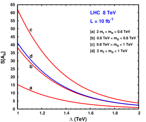
We show our results for some kinematic ranges of $m_{tt}$ and $\Lambda$ in the range $1\,{\rm TeV}<\Lambda<2\,{\rm TeV}$. The kinematic ranges of $m_{tt}$ considered in our analysis are the following

$$[{\rm a}] = 2\,m_{t}<m_{tt}<0.6\,{\rm TeV},$$ (17)

$$[{\rm b}] = 0.6\,{\rm TeV}<m_{tt}<0.8\,{\rm TeV},$$

$$[{\rm c}] = 0.8\,{\rm TeV}<m_{tt}<1\,{\rm TeV},$$

$$[{\rm d}] = 2\,m_{t}<m_{tt}<1\,{\rm TeV}\,.$$

The dashed lines correspond to the SM prediction at the LO in QCD. As we can see from the left plot in 3, the spin-correlation is positive for the [a] and [d] ranges, while it changes sign for the [b] and [c] range. Although we choose the convention Re$[g_{A}]>0$, the spin-correlation $A_{h}$ and cross sections do not depend on the sign[$g_{A}$].

As we can see from the results in Fig.3, the common trend of this scenario is a decrease of $A_{h}$ with respect to the SM prediction, while the corresponding SM deviations increase by selecting kinematic regions of $m_{tt}$ masses close to the scale $\Lambda$. This last property is due to the fact that the axial-vector form factor $g_{A}$ grows quadratically with $m_{tt}$. On the other hand, the common decrease from the SM prediction can be easily understood by looking at the definition of $A$ in Eq.(12) and at the polarized cross sections in Eqs.(8), (10). The gluon-gluon fusion mechanism dominates at the LHC energies with respect to the quark-antiquark annihilation process. In this case, $|g_{A}|$ enters only through the combination $\sigma^{gg}_{LR}+\sigma^{gg}_{RL}$ combination, since $\sigma^{gg}_{LL}$ and $\sigma^{gg}_{RR}$ do not depend on $g_{A}$. This results in a positive contribution to the total cross section (cfr. Eqs.(8) and (10)), but a negative one in the numerator of $A_{h}$, see Eq.(12), giving rise to a destructive contribution with respect to the SM one.

For the [a] and [d] ranges in the left plot of Fig.4, the maximum deviation from the SM value is obtained for $\Lambda=1$ TeV, corresponding to a 10% deviation from the SM prediction, while for the [b] and [c] ranges the effect is larger reaching almost a 25% and 100% deviations for the [c] and [d] ranges respectively. For values of $\Lambda=2$ TeV the overall NP effect is strongly reduced and $A_{h}$ results are much closer to the corresponding SM ones. The numerical values of $A_{h}$ in Fig.3 for $\Lambda=1$ TeV and $\Lambda=2$ TeV are $A_{h}=(30,-10,-40,22)$% and $A_{h}=(32,-2.1,-21,26)$% respectively. The four series of numbers reported in parenthesis will indicate from now on, if not differently specified, the results corresponding to the $m_{tt}$ integration ranges of [a],[b],[c],[d] respectively.

On the right plot of Fig.3, we show the corresponding statistical significance for $A_{h}$, that, following the definition of spin-correlation $A$ in (12), is

$$S[A_{h}] = \Delta A_{h}\sqrt{\sigma^{\rm SM+NP}L}\,,$$ (18)

where $\Delta A_{h}=|A_{h}^{\rm SM+NP}-A_{h}^{\rm SM}|$, $\sigma^{\rm SM+NP}$ is the total unpolarized cross section, and $L$ stands for the integrated luminosity, while the $\scriptstyle{\rm SM+NP}$ suffix stands for the full SM and NP contribution. In $\sigma^{\rm SM+NP}$ we have used the LO QCD cross sections. Notice that the significance in Eq.(18) is a simple theoretical estimation of the true one, since it does not take into account detector efficiencies, acceptance, resolution and systematics. From the results in the right plots of Fig.3, we can see that the corresponding significances for $L=10\,{\rm fb}^{-1}$ are quite large. In particular, for $\Lambda=1$ TeV and $\Lambda=2$ TeV we get $S[A_{h}]=(15,38,62,41)$ and $S[A_{h}]=(0.9,2.3,3.7,2.4)$ respectively. We can see that, for $\Lambda=2$ TeV, the significance is considerably lower, with the maximum effect $S[A_{h}]\simeq 4$ corresponding to the range [c]. Therefore, we stress that by analyzing the $m_{tt}$ distributions of $t\bar{t}$ spin correlations at the LHC, the full range up to $\Lambda\sim 2$ TeV can be probed at LHC 8 TeV, even with an integrated luminosity of $L=10\,{\rm fb}^{-1}$.

In Fig.4 we present the corresponding results of Fig.3, but for LHC energies of $\sqrt{S}=14$ TeV and integrated luminosity $L=10\,{\rm fb}^{-1}$.

Figure 4: Same as in Fig. 3 but for the LHC center of mass energy of 14 TeV and integrated luminosity L=10 fb^-1.

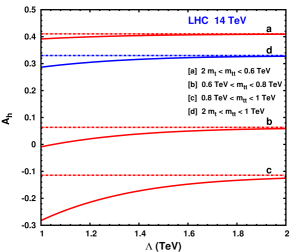
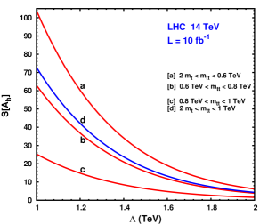
By increasing the LHC center of mass energy, we see that $|A_{h}|$ increases by roughly 25-30% with respect to the corresponding values at $\sqrt{S}=8$ TeV in the regions $A_{h}>0$, while it decreases of roughly the same amount in the regions $A_{h}<0$, for almost all the $m_{tt}$ ranges [a-d], including the SM values. In particular, we get $A_{h}=(39,-0.9,-28,28)\%$ and $A_{h}=(40,5.9,-12,33)\%$ for $\Lambda=1$ and $\Lambda=2$ TeV respectively, where the latter are quite close to the SM values. Due to the larger cross sections, the corresponding significances, with respect to the corresponding results at $\sqrt{S}=8$ TeV , are also increased, roughly by 70% and 30% effects for $\Lambda=1$ TeV and $\Lambda=2$ TeV respectively. In particular, we get $S[A_{h}]=(25,63,104,73)$ and $S[A_{h}]=(1.5,3.8,6.1,4.3)$ for $\Lambda=1$ TeV and $\Lambda=2$ TeV respectively.

3.2 Left-Right spin asymmetry

Here we consider the LR polarization asymmetry $A_{LR}$ defined as [99]

$$A_{LR} = \frac{N(\uparrow\uparrow)-N(\downarrow\downarrow)+N(\uparrow\downarrow)-N(\downarrow\uparrow)}{N(\uparrow\uparrow)+N(\downarrow\downarrow)+N(\uparrow\downarrow)+N(\downarrow\uparrow)},$$ (19)

where the left and right arrows denote the spins of the top and antitop respectively, with respect to a chosen quantization axis. As mentioned in the introduction, the SM contribution to this asymmetry ($A_{LR}^{\rm SM}$) is suppressed, being induced by one loop weak radiative corrections to the QCD $q\bar{q}\to t\bar{t}$ production. The typical SM value for $A_{LR}^{\rm SM}$ is very small, being of order of 0.5% and 0.04% for the cases of LHC 14 TeV and Tevatron respectively [99]. Therefore, this is a very sensitive probe to any potential parity-violating new physics beyond the SM. The LR polarization asymmetry has been analyzed in [95, 96, 97, 98] for the Tevatron and in [99, 100] for LHC, mainly in the framework of minimal supersymmetric extensions of the SM [99, 95, 96, 98] and more recently in more exotic NP scenarios like axigluons, third-generation enhanced LR models, and supersymmetric models without R-parity [100].

We will see that in our framework, the $A_{LR}$ is at least one order of magnitude larger than the corresponding SM contribution, since it is induced at the tree-level by the effect of the axial-vector coupling of the gluon. For this reason we will neglect the SM contribution to $A_{LR}$ in our analysis. Accordingly, we will use the following formula for the corresponding significance $S[A_{LR}]$

$$S[A_{LR}] = |A^{NP}_{LR}|\sqrt{\sigma^{\rm NP+SM}L}\,,$$ (20)

where in $A^{NP}_{LR}$ the leading contribution to the asymmetry is induced by the Re$[g_{A}]$ terms, which appears in the numerator of the right hand side of Eq.(19), while the denominator clearly includes the NP and SM contributions.

In the left plot of Fig.5 we present our results for the $A_{LR}$ calculated at the LO in QCD and in the helicity basis and laboratory frame, while on the right plot we show the corresponding significance $S[A_{LR}]$ for $L=10\,{\rm fb}^{-1}$.

Figure 5: Top-antitop left-right polarization asymmetry $A_{LR}$ (left plot) and corresponding significance $S[A_{LR}]$ (right plot) in $t\bar{t}$ events, in the helicity basis and laboratory frame, for the LHC center of mass energy of 8 TeV and integrated luminosity L=10 fb^-1, as a function of the scale $\Lambda$ and for some ranges of $m_{tt}$.

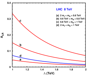
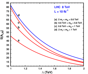
From these results we can see that the contribution induced by the pure axial-vector coupling to $A_{LR}$ is sizeable. In particular, for $\Lambda=1$ TeV, we get $A_{LR}=(4.5,15,33,7.2)$%, with a corresponding significance $S[A_{LR}]=(45,65,79,82)$, while for $\Lambda=2$ TeV the value of $A_{LR}$ lowers considerably, namely $A_{LR}=(1.1,3.4,7.2,1.6)$% with a corresponding significance $S[A_{LR}]=(11,14,15,18)$. From these results we can see that, although $A_{LR}$ is smaller than $A_{h}$, its statistical significance is higher than the corresponding one of $A_{h}$, mainly due to the fact that in the $A_{LR}$ the SM background is negligible. Therefore, $A_{LR}$ is a more sensitive probe of this scenario than $A_{h}$.

Notice that the sign of $A_{LR}$ in the right plot of Fig.5 depends on the convention we used for the sign of ${\rm Re}[g_{A}]$, namely positive. If we switch this sign, the asymmetry change sign too, being directly proportional to ${\rm Re}[g_{A}]$. Therefore, we stress that a non vanishing measurement of $A_{LR}$, also determines the sign of ${\rm Re}[g_{A}]$ in the framework of this scenario.

In Fig. 6 we show the corresponding results of $A_{LR}$ for LHC energy of $\sqrt{S}=14$ TeV.

Figure 6: Same as in Fig. 4 but for LHC center of mass energy of 14 TeV and integrated luminosity L=10 fb^-1.

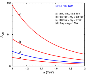
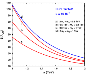
As we can see from the left plot of Fig.6, the trend of $A_{LR}$ by increasing the LHC energy is different with respect to the corresponding $A_{h}$ behavior, at fixed values of $\Lambda$. In particular, there is roughly a 45% decrease in $A_{LR}$, when passing from $\sqrt{S}=8$ TeV to 14 TeV. This is due to the fact that the total cross section, dominated by the gluon-gluon fusion process, grows faster than the $\sigma^{qq}_{LR}-\sigma^{qq}_{RL}$ contribution, by increasing the center of mass energy. In particular, for the [a-d] $m_{tt}$ ranges we get $A_{LR}=(2.8,8.6,19,4.7)\%$ and $A_{LR}=(0.7,1.9,3.8,1)\%$ for $\Lambda=1$ TeV and $\Lambda=2$ TeV respectively.

On the other hand, by comparing the corresponding significances $S[A_{LR}]$ at $\sqrt{S}=8$ TeV and 14 TeV in the right plots of Figs.5 and 6 respectively, we see that there is an almost 30% increase of $S[A_{LR}]$ in all integration ranges [a-d], when passing from $\sqrt{S}=8$ TeV to 14 TeV.

3.3 Comparison with ATLAS and CMS results

Now we discuss the impact of this scenario on the $m_{tt}$ inclusive measurements of $A_{h}$ performed by ATLAS and CMS collaborations, corresponding to LHC data at $\sqrt{S}=$7 TeV. In particular, we are interested in estimating the maximum effect induced by the axial-vector coupling contribution to these inclusive observables at fixed values of $\Lambda$. As mentioned before, this can be done at the cost of introducing a new free parameter in addition to $\Lambda$, that should be understood as the upper bound on the $g_{A}$ form factor in the high $m_{tt}$ mass regions $m_{tt}\gg\Lambda$.

Dimensional analysis and unitarity arguments, suggest that the $g_{A}(q^{2})$ form factor should not grow with $|q^{2}|$ indefinitely and should tend at most to a constant value in the asymptotic limit $|q^{2}|\gg\Lambda^{2}$, where in our case this corresponds to $q^{2}=m_{tt}^{2}\gg\Lambda^{2}$. In order to implement this parametrization, we replace $g_{A}$ in Eq.(5) by some test function $g_{A}(q^{2})=G_{F}(q^{2})$ , that reproduces the low energy limit in Eq.(5), but satisfies the asymptotic condition $\lim_{|q^{2}|\to\infty}\{g_{A}(q^{2})\}=\bar{g}_{A}$, where $\bar{g}_{A}$ is some constant. By naturalness arguments, we expect $\bar{g}_{A}$ to be at the most of order ${\cal O}(1)$. For simplifying the analysis, we will restrict to the case in which the constant $\bar{g}_{A}$ is real.

Basically, $\bar{g}_{A}$ plays the role here of a new dimensionless free parameter that parametrizes the upper bound of the axial-vector form factor $g_{A}$, in the kinematic regions $m_{tt}\gg\Lambda$. By using some test functions for the $g_{A}$ form factor, satisfying the above criteria, we will show that for $\Lambda>1$ TeV, deviations from the SM results in the inclusive $A_{h}$ values are very small, at most of order of 10% for asymptotic values of $\bar{g}_{A}\leq 10$.

As a toy model, we will use the following function to parametrizes the form factor $g_{A}(q^{2})=G_{F}(x)$, as a function of $x=q^{2}/\Lambda^{2}$, namely

$$G_{F}(x) = \bar{g}_{A}-\log{\left(\frac{e^{\bar{g}_{A}}+y}{1+y}\right)},{\rm with}~{}~{}~{}y\,=\,\frac{xe^{\bar{g}_{A}}}{(e^{\bar{g}_{A}}-1)}\,,$$ (21)

where $G_{F}(x)$ satisfies the required conditions $G_{F}(x)=x+{\cal O}(x^{2})$ for $x\ll 1$ and $\lim_{x\to\infty}G_{F}(x)=\bar{g}_{A}$. In Fig.7, we plot for comparison $G_{F}(x)$, evaluated at $\bar{g}_{A}=1$, with the function $G_{\theta}(x)$ defined as $G_{\theta}(x)=x\theta(1-x)+\bar{g}_{A}\theta(x-1)$.

Figure 7: The $G_{F}(x)$, evaluated at $\bar{g}_{A}=1$, and $G_{\theta}(x)$ versus $x=\hat{s}/\Lambda^{2}$.

Figure 8: The $m_{tt}$ inclusive values for $A_{h}$ (left) and $A_{LR}$ (right) respectively, for the LHC 7 TeV energy and $\Lambda=1$ TeV, versus the gluon axial-vector coupling cut-off $\bar{g}_{A}$. In left plot, colored (dark blue) bands stand for the ATLAS (top region) and CMS (down region) 2$\sigma$ regions, while the middle (light blue) band is the overlap between these two areas. The dashed dot and continuous (red) lines correspond to the SM prediction in Eq.(15) at the NLO in QCD and to the prediction of our scenario for the $G_{F}$ function respectively, all multiplied by the NLO rescaling factor.

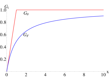
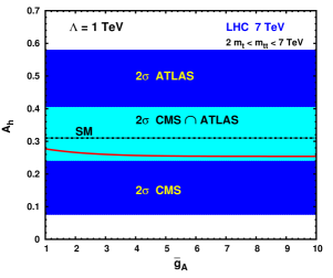
In the left plot of Fig.8 we show our prediction for the $m_{tt}$ inclusive spin correlation observable $A_{h}$ corresponding to $\Lambda=1$ TeV and LHC energy of 7 TeV, as a function of $\bar{g}_{A}$, for the $G_{F}(x)$ function. The colored bands stand for the 2$\sigma$ regions for the ATLAS (top region) [46] and CMS (down region) [47] measurements of $A_{h}$, while the middle band is the overlap between these two areas. The dashed dot and continuous (red) lines correspond to the SM prediction in Eq.(15) at the NLO in QCD and to the prediction of our scenario for the $G_{F}$ function respectively, suitably rescaled to the SM value at the NLO. In rescaling our predictions we multiplied the results obtained at the LO in QCD by the SM $K$ factor for the spin correlation defined as $K=A^{\rm NLO}_{h}/A^{\rm LO}_{h}$ at $\sqrt{S}=7$ TeV.

As we can see from these results, the impact of this scenario on the inclusive observable $A_{h}$ is a decrease of the $A_{h}$ values with respect to the SM prediction. In the region $4<\bar{g}_{A}<10$, the $A_{h}$ approaches to a plateau, namely $A_{h}\sim 25\%$. The expected deviations from the SM prediction, for $\Lambda=1$ TeV, are within the 2$\sigma$ bands of ATLAS and CMS measurements. If we consider larger values of the scale $\Lambda>1$ TeV, the SM deviations are dramatically reduced. The variation ($\delta A_{h}$) of $A_{h}$ in the range $1<\bar{g}_{A}<10$ is of order of $\delta A_{h}\sim 12$%, corresponding to $A_{h}=28$% and $A_{h}=25$%, for $\bar{g}_{A}=1$ and $\bar{g}_{A}=10$ respectively. The range of this variation should be interpreted as the theoretical uncertainty of our scenario on the inclusive observables, at fixed value of $\Lambda=1$ TeV, that becomes smaller by taking larger values of $\Lambda$. In the case of the total cross sections, this deviation is even smaller, being of the order of 0.8%, which is a very negligible effect in comparison to the other (QCD and PDF) uncertainties affecting the strong interactions induced cross sections at the LHC.

Moreover, the results in Fig.8 are not very sensitive to the choice of the parametrization function. For instance, for $\bar{g}_{A}=1$, the difference for $A_{h}$ evaluated by using $G_{F}(x)$ or $G_{\theta}(x)$ is of order of 8%.

In conclusion, we believe that this scenario and in particular the $\Lambda=1-1.3$ TeV region that is required to explain the Tevatron anomaly, is still consistent with the inclusive measurements of $A_{h}$ reported by the CMS and ATLAS collaborations within 2 standard deviations. This suggests that a dedicated experimental analysis of the $m_{tt}$ distributions of $A_{h}$ by the CMS and ATLAS collaboration is needed in order to either confirm or ruled out this scenario.

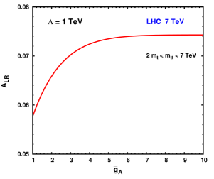
On the right plot of Fig.8 we show the corresponding predictions for the $m_{tt}$ inclusive observable $A_{LR}$. We can see that the general trend is an increase of the $A_{LR}$ values by increasing $\bar{g}_{A}$. We did not show the SM prediction in the plot since this is about one order of magnitude smaller. We can see that the $A_{LR}$ approaches to a constant value for $4<\bar{g}_{A}<10$, namely $A_{LR}=7.4$%. The variation of $A_{LR}$ in the considered range of $\bar{g}_{A}$, is of the order of $28$%, passing from 5.8% to 7.4%. Therefore, measurements of $A_{LR}$ at the LHC, even if inclusive in $m_{tt}$, could be crucial for testing this model, although a dedicated analysis of the $m_{tt}$ spectrum would be more effective and less model-dependent in constraining this scenario.

4 Conclusions

We have analyzed the impact of the gluon effective axial-vector coupling on the spin correlations $A_{h}$ and LR spin asymmetry $A_{LR}$ in top- antitop-quark production at the LHC. We studied these observables at different invariant masses of the $t\bar{t}$ system and showed that it would be necessary to measure these quantities as function of the $t\bar{t}$ invariant mass $m_{tt}$ at the LHC. In particular, we found that these observables are very sensitive to the NP scale $\Lambda$ associated with the effective axial-vector coupling of gluon, in the high $t\bar{t}$ invariant mass regions close enough to the scale $\Lambda$. Moreover, we found that the $A_{LR}$ is the best probe to test this scenario at the LHC since the SM background is negligible.

We estimated the potential effect of the gluon effective axial-vector coupling on the $m_{tt}$ inclusive spin correlations measurements obtained by ATLAS and CMS collaboration. We show that this scenario, for a scale $\Lambda\geq 1$ TeV, is still consistent with present measurements within standard deviations. Therefore, a more dedicated analysis of those quantities as a function of $m_{tt}$ is mandatory in order to test this scenario at the LHC. We stress that the 8 TeV LHC has enough sensitivity either to confirm the Tevatron top charge asymmetry anomaly or to rule it out in the context of the considered NP scenario.

Acknowledgements
We acknowledge useful discussions with W. Bernreuther and Z.-G. Si. E.G. would like to thank the PH-TH division of CERN for its kind hospitality during the preparation of this work. This work was supported by the ESF grants 8090, 8499, 8943, MTT8, MTT59, MTT60, MJD140, JD164, MJD298, by the recurrent financing SF0690030s09 project and by the European Union through the European Regional Development Fund.

Appendix A Matrix elements

Here we give the matrix elements for all possible helicity configurations of the initial and final state particles in partonic processes

$$q(k)\,\bar{q}(k^{\prime}) \to t(p_{t})\,\bar{t}(p_{\bar{t}})\,,$$ (22)

$$g(k)\,g(k^{\prime}) \to t(p_{t})\,\bar{t}(p_{{\bar{t}}})\,,$$ (23)

where $k,(k^{\prime})$ and $p_{t},(p_{\bar{t}})$ denote 4-momenta of the quark (antiquark) or gluon (gluon) initial and top- (antitop)-quark final states, respectively. The calculations were performed in the zero momentum frame (ZMF), where the $z$-axis was chosen in the direction of the top and all other momenta are assumed to lie on the $xz$-plane. In this frame the momenta 4-vectors for the top and antitop are

$$p_{t}=\frac{\sqrt{s}}{2}(1,0,0,\beta),\qquad p_{\bar{t}}=\frac{\sqrt{s}}{2}(1,0,0,-\beta),$$ (24)

where $\hat{s}=(p_{\bar{t}}+p_{t})^{2}$ and $\beta=\sqrt{1-4m_{t}^{2}/s}$. We compute the matrix elements for all possible helicity configurations of the initial and final particles. The spinors of helicity eigenstates are constructed by the helicity prescription, where the spin is given in the rest frame of the particle. The state is then boosted in the positive direction of the $z$-axis and then rotated clockwise in the $xz$-plane to end up with the chosen 4-momentum of the particle in the ZMF frame.

The cross-section is given by

$$\frac{\mathrm{d}\sigma^{i}}{\mathrm{d}\Omega} = \frac{\beta}{4\hat{s}}\alpha_{S}^{2}c^{i}|\tilde{\mathcal{M}}^{i}|^{2}\,,$$ (25)

where $i\in\{q\bar{q},gg\}$, $c^{i}$ is an overall group theoretic factor and $|\tilde{\mathcal{M}}^{i}|^{2}$ is a non-normalized color averaged squared amplitude for the process. It can be expressed as

$$|\tilde{\mathcal{M}}^{i}|^{2} = \rho_{hh^{\prime}}\bar{\rho}_{\bar{h}\bar{h}^{\prime}}R^{i}_{hh^{\prime},\bar{h}\bar{h}^{\prime}}\,.$$ (26)

Here $R$ describes the production of on-shell top quark pairs from a given initial state. The matrices $\rho$, $\bar{\rho}$ are the density matrices describing the measurement of polarized top and antitop quarks in specific final states. The subscripts $h$ and $\bar{h}$ in Eq. (26) denote the top and antitop helicities. In the chosen basis for spin states $\rho=(1+n^{i}_{t}\sigma_{i})/2$ and $\bar{\rho}=(1+n^{i}_{t}\sigma_{3}\sigma_{i}\sigma_{3})/2$, where $\sigma_{i}$ are Pauli matrices. The corresponding covariant spin vectors are

$$s_{t}=(\gamma\beta\,n_{t3},n_{t1},n_{t2},\gamma\,n_{t3}),\qquad s_{\bar{t}}=(\gamma\beta\,n_{\bar{t}3},-n_{\bar{t}1},n_{\bar{t}2},-\gamma\,n_{\bar{t}3}),$$ (27)

with $\gamma=\sqrt{s}/2m_{t}$. Helicity eigenstates correspond to $\vec{n}=(0,0,h)$ for both top and antitop, where $h$ is the sign of helicity. It takes values $+1$ and $-1$ denoting right-handed and left-handed fermions, respectively.

A.1 Polarized $q\bar{q}\to t\bar{t}$ process

The group theoretic factor for this process is

$$c^{q\bar{q}} = \frac{1}{4d(F)^{2}}d(A)\,=\,\frac{N^{2}-1}{4N^{2}},$$ (28)

where $d(F)=N$ and $d(A)=N^{2}-1$ are the dimensions of the fundamental (F) and adjoint (A) representation, respectively. The momenta of the initial quark and antiquark are

$$k = \frac{\sqrt{s}}{2}(1,-\sin(\theta)\beta_{q},0,\cos(\theta)\beta_{q}),\qquad k^{\prime}\,=\,\frac{\sqrt{s}}{2}(1,\sin(\theta)\beta_{q},0,-\cos(\theta)\beta_{q}),$$ (29)

where $\theta$ the is the angle between the momenta of the initial quark and top in the ZMF and $\beta_{q}=\sqrt{1-4m_{q}^{2}/s}$.

The squared matrix element is given by (25). For the initial $q\bar{q}$ the production matrix for a given initial state is

$$R^{q\bar{q}}_{hh^{\prime},\bar{h}\bar{h}^{\prime};h_{q}h_{\bar{q}}} =\tilde{\mathcal{M}}^{q\bar{q}*}_{h^{\prime}\bar{h}^{\prime};h_{q}h_{\bar{q}}}\tilde{\mathcal{M}}^{q\bar{q}}_{h\bar{h};h_{q}h_{\bar{q}}},$$ (30)

where

$$\tilde{\mathcal{M}}^{q\bar{q}}_{h\bar{h};h_{q}h_{\bar{q}}} = \delta_{h,\bar{h}}\delta_{h_{q},h_{\bar{q}}}\gamma_{q}^{-1}\gamma^{-1}\cos(\theta)$$ (31)

$$+ \delta_{h,\bar{h}}\delta_{h_{q},-h_{\bar{q}}}\gamma^{-1}\left(1+h_{q}g_{A}\beta_{q}\right)(-h_{q})\sin(\theta)$$

$$+ \delta_{h,-\bar{h}}\delta_{h_{q},h_{\bar{q}}}\gamma_{q}^{-1}\left(1+hg_{A}\beta\right)(+h)\sin(\theta)$$

$$+ \delta_{h,-\bar{h}}\delta_{h_{q},-h_{\bar{q}}}\left(1+h_{q}g_{A}\beta_{q}\right)\left(1+hg_{A}\beta\right)(1+h_{q}h\cos(\theta)),$$

where $\beta=\sqrt{1-4m_{t}^{2}/s}$, $\gamma=\sqrt{s}/2m_{t}$, and $\gamma_{q}=\sqrt{s}/2m_{q}$.

After taking the spin sum over initial polarizations, the squared matrix element can be given by:

$$\frac{1}{4}\sum_{h_{q},\bar{h}_{q}}|\tilde{\mathcal{M}}^{q\bar{q}}|^{2} = \mathcal{C}_{0}^{q\bar{q}}+n_{t}^{1}n_{\bar{t}}^{1}\mathcal{C}_{1}^{q\bar{q}}+n_{t}^{2}n_{\bar{t}}^{2}\mathcal{C}_{2}^{q\bar{q}}+n_{t}^{3}n_{\bar{t}}^{3}\mathcal{C}_{3}^{q\bar{q}}$$ (32)

$$+ (n_{t}^{1}n_{\bar{t}}^{3}+n_{\bar{t}}^{1}n_{t}^{3})\mathcal{C}_{13}^{q\bar{q}}+(-n_{t}^{1}+n_{\bar{t}}^{1})\mathcal{C}_{01}^{q\bar{q}}+(n_{t}^{3}-n_{\bar{t}}^{3})\mathcal{C}_{03}^{q\bar{q}}\,,$$

where

$$\mathcal{C}_{0}^{q\bar{q}} = \frac{1}{8}\Big{(}2(1+g_{A}^{2}\beta_{q}^{2})(1+g_{A}^{2}\beta^{2})+(1+g_{A}^{2}\beta_{q}^{2}+\gamma_{q}^{-2})(1+g_{A}^{2}\beta^{2}+\gamma^{-2})$$ (33)

$$+ \beta_{q}^{2}\beta^{2}(1+g_{A}^{2})^{2}\cos(2\theta)\Big{)}+2\beta_{q}\beta g_{A}^{2}\cos(\theta)\,,$$

$$\mathcal{C}_{1}^{q\bar{q}} = -\frac{1}{4}\Big{(}\gamma_{q}^{-2}\gamma^{-2}+\beta_{q}^{2}(1+g_{A}^{2})(1-g_{A}^{2}\beta^{2}+\gamma^{-2})\sin^{2}(\theta)\Big{)},$$ (34)

$$\mathcal{C}_{2}^{q\bar{q}} = -\frac{1}{4}\Big{(}-\gamma_{q}^{-2}\gamma^{-2}+\beta_{q}^{2}(1+g_{A}^{2})(1-g_{A}^{2}\beta^{2}-\gamma^{-2})\sin^{2}(\theta)\Big{)}\,,$$ (35)

$$\mathcal{C}_{3}^{q\bar{q}} = -\frac{1}{8}\Big{(}2(1+g_{A}^{2}\beta_{q}^{2})(1+g_{A}^{2}\beta^{2})+(1+g_{A}^{2}\beta_{q}^{2}+\gamma_{q}^{-2})\beta^{2}(1+g_{A}^{2})$$ (36)

$$+ \beta_{q}^{2}(1+g_{A}^{2})(1+g_{A}^{2}\beta^{2}+\gamma^{-2})\cos(2\theta)\Big{)}-2\beta_{q}\beta g_{A}^{2}\cos(\theta)\,,$$

$$\mathcal{C}_{13}^{q\bar{q}} = \gamma^{-1}\beta_{q}\Big{(}\beta g_{A}^{2}+\frac{1}{2}\beta_{q}(1+g_{A}^{2})\cos(\theta)\Big{)}\sin(\theta)\,,$$ (37)

$$\mathcal{C}_{01}^{q\bar{q}} = \gamma^{-1}\beta_{q}g_{A}\Big{(}1+\frac{1}{2}\beta_{q}\beta(1+g_{A}^{2})\cos(\theta)\Big{)}\sin(\theta)\,,$$ (38)

$$\mathcal{C}_{03}^{q\bar{q}} = g_{A}\left(\beta+\beta_{q}(1+g_{A}^{2}\beta^{2})\cos(\theta)+\beta_{q}^{2}\beta\left(g_{A}^{2}-\frac{1}{2}(1+g_{A}^{2})\sin^{2}(\theta)\right)\right)\,.$$ (39)

The coefficient $\mathcal{C}_{0}$ is proportional to the (final) spin summed result. The quotients $\mathcal{C}_{i}/\mathcal{C}_{0}$, $i\in\{1,2,3\}$ give spin correlations and the quotients $\mathcal{C}_{i}/\mathcal{C}_{0}$, $i\in\{01,03\}$ give the spin asymmetry for the corresponding quantization axis. Direction ”3” corresponds to helicity. The term $\mathcal{C}_{03}^{q\bar{q}}$ is the only source of the spin asymmetry (19) at tree level.

The phase space integration is performed over the solid angle. The spin parameters $n^{1}_{t}$, $n^{2}_{t}$, $n^{1}_{t}$, $n^{2}_{t}$ are implicitly dependent on the azimuthal angle, so terms linear in these parameters vanish. Therefore the coefficients $\mathcal{C}_{01}$ and $\mathcal{C}_{13}$ do not contribute to the total cross-section. Only the sum $\mathcal{C}_{1}+\mathcal{C}_{2}$ is relevant after the phase space integration. In conclusion

$$\frac{1}{4\pi}\int|\tilde{\mathcal{M}}^{q\bar{q}}|^{2}\,\mathrm{d}\Omega = \mathcal{I}_{0}^{q\bar{q}}+(n_{t}^{1}n_{\bar{t}}^{1}+n_{t}^{2}n_{\bar{t}}^{2})\,\mathcal{I}_{1+2}^{q\bar{q}}+n_{t}^{3}n_{\bar{t}}^{3}\,\mathcal{I}_{3}^{q\bar{q}}+(n_{t}^{3}-n_{\bar{t}}^{3})\,\mathcal{I}_{03}^{q\bar{q}}\,,$$ (40)

where

$$\mathcal{I}_{0}^{q\bar{q}} = \frac{1}{3}(1+g_{A}^{2}\beta_{q}^{2}+\gamma_{q}^{-2}/2)(1+g_{A}^{2}\beta^{2}+\gamma^{-2}/2)\,,$$ (41)

$$\mathcal{I}_{1+2}^{q\bar{q}} = -\frac{1}{3}(1+g_{A}^{2}\beta_{q}^{2}+\gamma_{q}^{-2}/2)(1-g_{A}^{2}\beta^{2})\,,$$ (42)

$$\mathcal{I}_{3}^{q\bar{q}} = -\frac{1}{3}(1+g_{A}^{2}\beta_{q}^{2}+\gamma_{q}^{-2}/2)(1+g_{A}^{2}\beta^{2}-\gamma^{-2}/2)\,,$$ (43)

$$\mathcal{I}_{03}^{q\bar{q}} = \frac{2}{3}(1+g_{A}^{2}\beta_{q}^{2}+\gamma_{q}^{-2}/2)g_{A}\beta\,.$$ (44)

A.2 Polarized $gg\to t\bar{t}$ process

The group theoretic overall factor for this process is

$$c^{gg} = \frac{d(F)C_{F}^{2}}{d(A)^{2}}\,=\,\frac{1}{4N}\,,$$ (45)

where $C_{F}=\frac{N^{2}-1}{2N}$ is the quadratic Casimir invariant of the fundamental representation. The gluon momenta are $k=\frac{\sqrt{s}}{2}(1,-\sin(\theta),0,\cos(\theta))$ and $k^{\prime}=\frac{\sqrt{s}}{2}(1,\sin(\theta),0,-\cos(\theta))$, where $\theta$ the is the angle between gluon and top momenta in the ZMF. The corresponding spin polarization vectors are $\epsilon_{\pm}=\frac{1}{\sqrt{2}}(1,\mp\sin(\theta),i,\mp\cos(\theta))$.

The production matrix takes a form

$$R^{gg}_{hh^{\prime},\bar{h}\bar{h}^{\prime};\lambda_{g}\lambda^{\prime}_{g}} =4\begin{pmatrix}\tilde{\mathcal{M}}^{tu}_{h^{\prime}\bar{h}^{\prime};\lambda_{g}\lambda^{\prime}_{g}}\\ \tilde{\mathcal{M}}^{g}_{h^{\prime}\bar{h}^{\prime};\lambda_{g}\lambda^{\prime}_{g}}\end{pmatrix}^{\dagger}\begin{pmatrix}\mathcal{A}(\mathcal{A}-C_{r})&\mathcal{A}\beta\cos(\theta)C_{r}\\ \mathcal{A}\beta\cos(\theta)C_{r}&C_{r}\\ \end{pmatrix}\begin{pmatrix}\tilde{\mathcal{M}}^{tu}_{h\bar{h};\lambda_{g}\lambda^{\prime}_{g}}\\ \tilde{\mathcal{M}}^{g}_{h\bar{h};\lambda_{g}\lambda^{\prime}_{g}}\,,\end{pmatrix},$$ (46)

where $\mathcal{A}=(1-\beta^{2}\cos^{2}(\theta))^{-1}$ and

$$C_{r} = \frac{C_{2}(G)}{4C_{F}}\,=\,\frac{N^{2}}{2(N^{2}-1)}\,,$$ (47)

is a group theoretic constant, $0\leq C_{r}\leq 1$, with $C_{2}(G)=N$ being the quadratic Casimir invariant in the adjoint representation. $C_{r}$ is independent of the normalization of the group generators and for Abelian groups $C_{r}=0$. For abelian gauge theories $R$ is determined entirely by $\tilde{\mathcal{M}}^{tu}$, as one would expect.

For gluon spins $\lambda_{g}$ and $\lambda^{\prime}_{g}$ the amplitudes $\tilde{\mathcal{M}}^{tu}$ and $\tilde{\mathcal{M}}^{g}$ are

$$\tilde{\mathcal{M}}^{tu}_{h\bar{h};\lambda_{g}\lambda^{\prime}_{g}} = \delta_{h,\bar{h}}\delta_{\lambda_{g},\lambda^{\prime}_{g}}\ \ \gamma^{-1}\beta\sin^{2}(\theta)$$ (48)

$$- \delta_{h,\bar{h}}\delta_{\lambda_{g},-\lambda^{\prime}_{g}}\ \gamma^{-1}(h\lambda_{g}+\beta)$$

$$- \delta_{h,-\bar{h}}\delta_{\lambda_{g},\lambda^{\prime}_{g}}\ \beta(\lambda_{g}+h\cos(\theta))\sin(\theta),$$

$$\tilde{\mathcal{M}}^{g}_{h\bar{h};\lambda_{g}\lambda^{\prime}_{g}} = \delta_{h,-\bar{h}}\delta_{\lambda_{g},-\lambda^{\prime}_{g}}\ g_{A}\beta\sin(\theta)\,.$$ (49)

The axial coupling appears only in the non-abelian part $\tilde{\mathcal{M}}^{g}$ when top-quarks with opposite helicity are produced from gluons with opposite spin. The effect disappears for low energies and collinear momenta.

After taking the spin average over initial polarizations, the squared matrix element can be given in a relatively compact form:

$$\frac{1}{4}\sum_{\lambda_{g},\lambda^{\prime}_{g}}|\tilde{\mathcal{M}}^{gg}|^{2} = \mathcal{C}_{0}^{gg}+n_{t}^{1}n_{\bar{t}}^{1}\mathcal{C}_{1}^{gg}+n_{t}^{2}n_{\bar{t}}^{2}\mathcal{C}_{2}^{gg}+n_{t}^{3}n_{\bar{t}}^{3}\mathcal{C}_{3}^{gg}$$ (50)

$$+ (n_{t}^{1}n_{\bar{t}}^{3}+n_{\bar{t}}^{1}n_{t}^{3})\mathcal{C}_{13}^{gg}+(-n_{t}^{1}+n_{\bar{t}}^{1})\mathcal{C}_{01}^{gg}\,,$$

where

$$\mathcal{C}_{0}^{gg} = \mathcal{A}(\mathcal{A}-C_{r})[1-\beta^{4}(1+\sin^{4}(\theta))+2\beta^{2}\sin^{2}(\theta)]+C_{r}g_{A}^{2}\beta^{2}\sin^{2}(\theta)\,,$$ (51)

$$\mathcal{C}_{1}^{gg} = -\mathcal{A}(\mathcal{A}-C_{r})[-\gamma^{-4}+(1-\gamma^{-4})\sin^{4}(\theta)]-C_{r}g_{A}^{2}\beta^{2}\sin^{2}(\theta)\,,$$ (52)

$$\mathcal{C}_{2}^{gg} = -\mathcal{A}(\mathcal{A}-C_{r})[\gamma^{-4}+\beta^{4}\sin^{4}(\theta)]-C_{r}g_{A}^{2}\beta^{2}\sin^{2}(\theta)\,,$$ (53)

$$\mathcal{C}_{3}^{gg} = \mathcal{A}(\mathcal{A}-C_{r})[1-\beta^{4}(1+\sin^{4}(\theta))-2\beta^{2}\sin^{2}(\theta)\cos^{2}(\theta)]-C_{r}g_{A}^{2}\beta^{2}\sin^{2}(\theta)\,,$$ (54)

$$\mathcal{C}_{13}^{gg} = \mathcal{A}(\mathcal{A}-C_{r})\gamma^{-1}\beta^{2}\sin(2\theta)\sin^{2}(\theta)\,,$$ (55)

$$\mathcal{C}_{01}^{gg} = C_{r}\mathcal{A}g_{A}\gamma^{-1}\beta^{3}\sin(2\theta)\,.$$ (56)

The coefficient $\mathcal{C}_{0}$ is proportional to the (final) spin summed result and the rest are associated with different spin observables. Note that there is no LR-asymmetry for the $gg$-initial state, because there is no term similar to Eq.(39). Instead, in this process the axial coupling introduces another strong spin asymmetry that is not present in the standard model. It is induced by the coefficient $\mathcal{C}_{01}^{gg}$ (and similarly by $\mathcal{C}_{01}^{q\bar{q}}$ (38) for the $q\bar{q}$ initial state). This term is caused by the interference between the axial-vector and the vector couplings, and it is the only term of this kind for the $gg$ initial state. This term could induce azimuthal asymmetries. However, for the symmetric initial state, this effect averages out. In order to observe a physical azimuthal asymmetry induced by $\mathcal{C}_{01}^{gg}$, initial state polarization is needed.

The phase space averaged squared matrix element is given by

$$\frac{1}{4\pi}\int|\tilde{\mathcal{M}}^{gg}|^{2}\,\mathrm{d}\Omega = \mathcal{I}_{0}^{q\bar{q}}+(n_{t}^{1}n_{\bar{t}}^{1}+n_{t}^{2}n_{\bar{t}}^{2})\,\mathcal{I}_{1+2}^{gg}+n_{t}^{3}n_{\bar{t}}^{3}\,\mathcal{I}_{3}^{gg}\,,$$ (57)

where

$$\mathcal{I}_{0}^{gg} = -\frac{1}{16}\left(28+31\gamma^{-2}-(32+32\gamma^{-2}+2\gamma^{-4})\frac{\alpha}{\beta}\right)+\frac{3}{8}g_{A}^{2}\beta^{2}\,,$$ (58)

$$\mathcal{I}_{1+2}^{gg} = -\frac{1}{16\beta^{2}}\left(10+23\gamma^{-2}-\gamma^{-2}(32+\gamma^{-2})\frac{\alpha}{\beta}\right)-\frac{3}{8}g_{A}^{2}\beta^{2}\,,$$ (59)

$$\mathcal{I}_{3}^{gg} = \frac{1}{16\beta^{2}}\left(60-25\gamma^{-2}+31\gamma^{-4}-(32+4\gamma^{-2}+28\gamma^{-4}+2\gamma^{-6})\frac{\alpha}{\beta}\right)-\frac{3}{8}g_{A}^{2}\beta^{2}\,,$$ (60)

where $\alpha=\mathrm{atanh}(\beta)$ is the rapidity and the substitution $C_{r}=9/16$ corresponding to SU(3) was made.

References

- [1] M. Beneke, I. Efthymiopoulos, M. L. Mangano, J. Womersley, A. Ahmadov, et al.(2000), arXiv:hep-ph/0003033 [hep-ph]
- [2] S. Abachi et al. (D0 Collaboration), Phys.Rev.Lett. 74, 2422
- [3] F. Abe et al. (CDF Collaboration), Phys.Rev.Lett. 74, 2626 (1995), arXiv:hep-ex/9503002 [hep-ex]
- [4] F.-P. Schilling, Int.J.Mod.Phys. A27, 1230016 (2012), arXiv:1206.4484 [hep-ex]
- [5] J. Beringer et al. (Particle Data Group), Phys.Rev. D86, 010001 (2012)
- [6] P. Nason, S. Dawson, and R. K. Ellis, Nucl.Phys. B303, 607 (1988)
- [7] P. Nason, S. Dawson, and R. K. Ellis, Nucl.Phys. B327, 49 (1989)
- [8] W. Beenakker, H. Kuijf, W. van Neerven, and J. Smith, Phys.Rev. D40, 54 (1989)
- [9] W. Beenakker, W. van Neerven, R. Meng, G. Schuler, and J. Smith, Nucl.Phys. B351, 507 (1991)
- [10] M. L. Mangano, P. Nason, and G. Ridolfi, Nucl.Phys. B373, 295 (1992)
- [11] E. Laenen, J. Smith, and W. van Neerven, Phys.Lett. B321, 254 (1994), arXiv:hep-ph/9310233 [hep-ph]
- [12] S. Frixione, M. L. Mangano, P. Nason, and G. Ridolfi, Phys.Lett. B351, 555 (1995), arXiv:hep-ph/9503213 [hep-ph]
- [13] N. Kidonakis and G. F. Sterman, Nucl.Phys. B505, 321 (1997), arXiv:hep-ph/9705234 [hep-ph]
- [14] R. Bonciani, S. Catani, M. L. Mangano, and P. Nason, Nucl.Phys. B529, 424 (1998), arXiv:hep-ph/9801375 [hep-ph]
- [15] N. Kidonakis, E. Laenen, S. Moch, and R. Vogt, Phys.Rev. D64, 114001 (2001), arXiv:hep-ph/0105041 [hep-ph]
- [16] M. Cacciari, S. Frixione, M. L. Mangano, P. Nason, and G. Ridolfi, JHEP 0809, 127 (2008), arXiv:0804.2800 [hep-ph]
- [17] S. Moch and P. Uwer, Phys.Rev. D78, 034003 (2008), arXiv:0804.1476 [hep-ph]
- [18] N. Kidonakis(2009), arXiv:0909.0037 [hep-ph]
- [19] V. Ahrens, M. Neubert, B. D. Pecjak, A. Ferroglia, and L. L. Yang, Phys.Lett. B703, 135 (2011), arXiv:1105.5824 [hep-ph]
- [20] N. Kidonakis(2011), arXiv:1105.3481 [hep-ph]
- [21] J. H. Kuhn, Nucl.Phys. B237, 77 (1984)
- [22] V. D. Barger, J. Ohnemus, and R. Phillips, Int.J.Mod.Phys. A4, 617 (1989)
- [23] G. L. Kane, G. Ladinsky, and C. Yuan, Phys.Rev. D45, 124 (1992)
- [24] T. Arens and L. Sehgal, Phys.Lett. B302, 501 (1993)
- [25] G. Mahlon and S. J. Parke, Phys.Rev. D53, 4886 (1996), arXiv:hep-ph/9512264 [hep-ph]
- [26] T. Stelzer and S. Willenbrock, Phys.Lett. B374, 169 (1996), arXiv:hep-ph/9512292 [hep-ph]
- [27] A. Brandenburg, Phys.Lett. B388, 626 (1996), arXiv:hep-ph/9603333 [hep-ph]
- [28] D. Chang, S.-C. Lee, and A. Sumarokov, Phys.Rev.Lett. 77, 1218 (1996), arXiv:hep-ph/9512417 [hep-ph]
- [29] W. Bernreuther, A. Brandenburg, and P. Uwer, Phys.Lett. B368, 153 (1996), arXiv:hep-ph/9510300 [hep-ph]
- [30] W. G. Dharmaratna and G. R. Goldstein, Phys.Rev. D53, 1073 (1996)
- [31] G. Mahlon and S. J. Parke, Phys.Lett. B411, 173 (1997), arXiv:hep-ph/9706304 [hep-ph]
- [32] P. Uwer, Phys.Lett. B609, 271 (2005), arXiv:hep-ph/0412097 [hep-ph]
- [33] W. Bernreuther, A. Brandenburg, Z. Si, and P. Uwer, Phys.Rev.Lett. 87, 242002 (2001), arXiv:hep-ph/0107086 [hep-ph]
- [34] W. Bernreuther, A. Brandenburg, Z. Si, and P. Uwer, Nucl.Phys. B690, 81 (2004), arXiv:hep-ph/0403035 [hep-ph]
- [35] W. Bernreuther and Z.-G. Si, Nucl.Phys. B837, 90 (2010), arXiv:1003.3926 [hep-ph]
- [36] G. Mahlon and S. J. Parke, Phys.Rev. D81, 074024 (2010), arXiv:1001.3422 [hep-ph]
- [37] R. Frederix and F. Maltoni, JHEP 0901, 047 (2009), arXiv:0712.2355 [hep-ph]
- [38] M. Arai, N. Okada, and K. Smolek, Phys.Rev. D79, 074019 (2009), arXiv:0902.0418 [hep-ph]
- [39] K.-m. Cheung, Phys.Rev. D55, 4430 (1997), arXiv:hep-ph/9610368 [hep-ph]
- [40] J.-Y. Liu, Z.-G. Si, and C.-X. Yue, Phys.Rev. D81, 015011 (2010)
- [41] S. S. Biswal, S. D. Rindani, and P. Sharma(2012), arXiv:1211.4075 [hep-ph]
- [42] T. Aaltonen et al. (CDF Collaboration), Phys.Rev. D83, 031104 (2011), arXiv:1012.3093 [hep-ex]
- [43] V. M. Abazov et al. (D0 Collaboration), Phys.Rev.Lett. 107, 032001 (2011), arXiv:1104.5194 [hep-ex]
- [44] V. M. Abazov et al. (D0 Collaboration), Phys.Lett. B702, 16 (2011), arXiv:1103.1871 [hep-ex]
- [45] V. M. Abazov et al. (D0 Collaboration), Phys.Rev.Lett. 108, 032004 (2012), arXiv:1110.4194 [hep-ex]
- [46] G. Aad et al. (ATLAS Collaboration), Phys.Rev.Lett. 108, 212001 (2012), arXiv:1203.4081 [hep-ex]
- [47] S. Chatrchyan et al. (CMS Collaboration)(2012), CMS-PAS-TOP-12-004
- [48] J. H. Kuhn and G. Rodrigo, Phys.Rev.Lett. 81, 49 (1998), arXiv:hep-ph/9802268 [hep-ph]
- [49] J. H. Kuhn and G. Rodrigo, Phys.Rev. D59, 054017 (1999), arXiv:hep-ph/9807420 [hep-ph]
- [50] M. Bowen, S. Ellis, and D. Rainwater, Phys.Rev. D73, 014008 (2006), arXiv:hep-ph/0509267 [hep-ph]
- [51] T. Aaltonen et al. (CDF Collaboration), Phys.Rev. D83, 112003 (2011), arXiv:1101.0034 [hep-ex]
- [52] V. M. Abazov et al. (D0 Collaboration)(2011), arXiv:1107.4995 [hep-ex]
- [53] T. Aaltonen et al. (The CDF Collaboration), Phys.Rev. D82, 052002 (2010), arXiv:1002.2919 [hep-ex]
- [54] V. Abazov et al. (D0 Collaboration), Phys.Lett. B679, 177 (2009), arXiv:0901.2137 [hep-ex]
- [55] Measurement of production in the all-hadronic channel in 1.02 of pp collisions at TeV with the ATLAS detector, Tech. Rep. ATLAS-CONF-2011-140 (CERN, Geneva, 2011)
- [56] Measurement of the ttbar production cross section in the fully hadronic decay channel in pp collisions at 7 TeV, Tech. Rep. CMS-PAS-TOP-11-007 (CERN, Geneva, 2011)
- [57] O. Antunano, J. H. Kuhn, and G. Rodrigo, Phys.Rev. D77, 014003 (2008), arXiv:0709.1652 [hep-ph]
- [58] P. Ferrario and G. Rodrigo, Phys.Rev. D78, 094018 (2008), arXiv:0809.3354 [hep-ph]
- [59] P. Ferrario and G. Rodrigo, Phys.Rev. D80, 051701 (2009), arXiv:0906.5541 [hep-ph]
- [60] P. H. Frampton, J. Shu, and K. Wang, Phys.Lett. B683, 294 (2010), arXiv:0911.2955 [hep-ph]
- [61] R. S. Chivukula, E. H. Simmons, and C.-P. Yuan, Phys.Rev. D82, 094009 (2010), arXiv:1007.0260 [hep-ph]
- [62] Y. Bai, J. L. Hewett, J. Kaplan, and T. G. Rizzo, JHEP 1103, 003 (2011), arXiv:1101.5203 [hep-ph]
- [63] X.-P. Wang, Y.-K. Wang, B. Xiao, J. Xu, and S.-h. Zhu, Phys.Rev. D83, 115010 (2011), arXiv:1104.1917 [hep-ph]
- [64] U. Haisch and S. Westhoff, JHEP 1108, 088 (2011), arXiv:1106.0529 [hep-ph]
- [65] J. Aguilar-Saavedra and M. Perez-Victoria, Phys.Lett. B705, 228 (2011), arXiv:1107.2120 [hep-ph]
- [66] G. Z. Krnjaic, Phys.Rev. D85, 014030 (2012), arXiv:1109.0648 [hep-ph]
- [67] J. Aguilar-Saavedra and J. Santiago, Phys.Rev. D85, 034021 (2012), arXiv:1112.3778 [hep-ph]
- [68] S. Jung, H. Murayama, A. Pierce, and J. D. Wells, Phys.Rev. D81, 015004 (2010), arXiv:0907.4112 [hep-ph]
- [69] B. Xiao, Y.-k. Wang, and S.-h. Zhu, Phys.Rev. D82, 034026 (2010), arXiv:1006.2510 [hep-ph]
- [70] J. Cao, L. Wang, L. Wu, and J. M. Yang, Phys.Rev. D84, 074001 (2011), arXiv:1101.4456 [hep-ph]
- [71] E. L. Berger, Q.-H. Cao, C.-R. Chen, C. S. Li, and H. Zhang, Phys.Rev.Lett. 106, 201801 (2011), arXiv:1101.5625 [hep-ph]
- [72] J. Aguilar-Saavedra and M. Perez-Victoria, Phys.Lett. B701, 93 (2011), arXiv:1104.1385 [hep-ph]
- [73] D.-W. Jung, P. Ko, and J. S. Lee, Phys.Rev. D84, 055027 (2011), arXiv:1104.4443 [hep-ph]
- [74] M. Duraisamy, A. Rashed, and A. Datta, Phys.Rev. D84, 054018 (2011), arXiv:1106.5982 [hep-ph]
- [75] P. Ko, Y. Omura, and C. Yu, Phys.Rev. D85, 115010 (2012), arXiv:1108.0350 [hep-ph]
- [76] K. Cheung, W.-Y. Keung, and T.-C. Yuan, Phys.Lett. B682, 287 (2009), arXiv:0908.2589 [hep-ph]
- [77] K. Cheung and T.-C. Yuan, Phys.Rev. D83, 074006 (2011), arXiv:1101.1445 [hep-ph]
- [78] B. Bhattacherjee, S. S. Biswal, and D. Ghosh, Phys.Rev. D83, 091501 (2011), arXiv:1102.0545 [hep-ph]
- [79] V. Barger, W.-Y. Keung, and C.-T. Yu, Phys.Lett. B698, 243 (2011), arXiv:1102.0279 [hep-ph]
- [80] N. Craig, C. Kilic, and M. J. Strassler, Phys.Rev. D84, 035012 (2011), arXiv:1103.2127 [hep-ph]
- [81] C.-H. Chen, S. S. Law, and R.-H. Li, J.Phys. G38, 115008 (2011), arXiv:1104.1497 [hep-ph]
- [82] K. Yan, J. Wang, D. Y. Shao, and C. S. Li, Phys.Rev. D85, 034020 (2012), arXiv:1110.6684 [hep-ph]
- [83] S. Knapen, Y. Zhao, and M. J. Strassler, Phys.Rev. D86, 014013 (2012), arXiv:1111.5857 [hep-ph]
- [84] S. Chatrchyan et al. (CMS Collaboration), JHEP 1108, 005 (2011), arXiv:1106.2142 [hep-ex]
- [85] V. Khachatryan et al. (CMS Collaboration), Phys.Rev.Lett. 106, 201804 (2011), arXiv:1102.2020 [hep-ex]
- [86] G. Aad et al. (ATLAS Collaboration), New J.Phys. 13, 053044 (2011), arXiv:1103.3864 [hep-ex]
- [87] E. Gabrielli and M. Raidal, Phys.Rev. D84, 054017 (2011), arXiv:1106.4553 [hep-ph]
- [88] M. Bohm, H. Spiesberger, and W. Hollik, Fortsch.Phys. 34, 687 (1986)
- [89] E. Gabrielli, M. Raidal, and A. Racioppi, Phys.Rev. D85, 074021 (2012), arXiv:1112.5885 [hep-ph]
- [90] J. H. Kuhn and G. Rodrigo(2011), arXiv:1109.6830 [hep-ph]
- [91] G. Rodrigo and P. Ferrario, Nuovo Cim. C033N4, 221 (2010), arXiv:1007.4328 [hep-ph]
- [92] Measurement of the Charge Asymmetry in Top Quark Pair Production, Tech. Rep. CMS-PAS-TOP-11-014 (CERN, Geneva, 2011)
- [93] S. Chatrchyan et al. (CMS Collaboration), Phys.Lett. B709, 28 (2012), arXiv:1112.5100 [hep-ex]
- [94] Measurement of the charge asymmetry in top quark pair production in pp collisions at sqrts=7 TeV using the ATLAS detector, Tech. Rep. ATLAS-CONF-2011-106 (CERN, Geneva, 2011)
- [95] C.-S. Li, R. J. Oakes, J. M. Yang, and C. Yuan, Phys.Lett. B398, 298 (1997), arXiv:hep-ph/9701350 [hep-ph]
- [96] C. S. Li, C. Yuan, and H.-Y. Zhou, Phys.Lett. B424, 76 (1998), arXiv:hep-ph/9709275 [hep-ph]
- [97] C. Kao, Phys.Lett. B348, 155 (1995), arXiv:hep-ph/9411337 [hep-ph]
- [98] Z. Sullivan, Phys.Rev. D56, 451 (1997), arXiv:hep-ph/9611302 [hep-ph]
- [99] C. Kao and D. Wackeroth, Phys.Rev. D61, 055009 (2000), arXiv:hep-ph/9902202 [hep-ph]
- [100] J. Cao, L. Wu, and J. M. Yang, Phys.Rev. D83, 034024 (2011), arXiv:1011.5564 [hep-ph]
- [101] W. Hollik and D. Pagani, Phys.Rev. D84, 093003 (2011), arXiv:1107.2606 [hep-ph]
- [102] P. Haberl, O. Nachtmann, and A. Wilch, Phys.Rev. D53, 4875 (1996), arXiv:hep-ph/9505409 [hep-ph]
- [103] Z. Hioki and K. Ohkuma, Eur.Phys.J. C65, 127 (2010), arXiv:0910.3049 [hep-ph]
- [104] K. Blum et al., Phys. Lett. B702, 364 (2011), arXiv:1102.3133 [hep-ph]
- [105] M. Raidal and A. Santamaria, Phys. Lett. B421, 250 (1998), arXiv:hep-ph/9710389
- [106] J. Pumplin, D. Stump, J. Huston, H. Lai, P. M. Nadolsky, et al., JHEP 0207, 012 (2002), arXiv:hep-ph/0201195 [hep-ph]