Strong correlations in density-functional theory: A model of spin-charge and spin-orbital separations

Abstract

It is known that the separation of electrons into spinons and chargons, the spin-charge separation, plays a decisive role when describing strongly correlated density distributions in one dimension [Phys. Rev. B 2012, 86, 075132]. In this manuscript, we extend the investigation by considering a model for the third electron fractionalization: the separation into spinons, chargons and orbitons – the last associated with the electronic orbital degree of freedom. Specifically, we deal with two exact constraints of exchange-correlation (XC) density-functionals: (i) The constancy of the highest occupied (HO) Kohn-Sham (KS) eigenvalues upon fractional electron numbers, and (ii) their discontinuities at integers. By means of one-dimensional (1D) discrete Hubbard chains and 1D H₂ molecules in the continuum, we find that spin-charge separation yields almost constant HO KS eigenvalues, whereas the spin-orbital counterpart can be decisive when describing derivative discontinuities of XC potentials at strong correlations.

1 Introduction

Spin and charge use to be treated as fundamental properties of ordinary electrons. However, when confined in one dimension, interacting electrons display the unusual property of separating their spin and charge into two independent quasiparticles: spinons and chargons.² Both behave just like ordinary electrons, but: spinons have spin-$1/2$ and no electrical charge, while chargons are spinless charged electrons. Recently,^{3, 4} an additional fractionalization was shown to occur: The spin-orbital separation, for which spin and orbital degrees of freedom are decoupled to form the orbitons – particles with no spin and charge, carrying solely the orbital information. Both, the spin-charge and spin-orbital separations have recent evidences of experimental observation,^{4, 5} teaching us that ordinary electrons can be considered bounded states of spinons, chargons and orbitons.

The Kohn-Sham (KS) formalism of density-functional theory (DFT),^{6, 7} by construction, retains the spin, charge and orbital degrees of freedom together, once it considers an auxiliary system of noninteracting particles. In contrast, it has been shown that the separation into spinons and chargons are decisive when dealing with strongly correlated density distributions in one dimension.⁸ W. Yang et. al. have assumed strongly correlated systems as one of the modern challenges for DFT: “The challenge of strongly correlated systems is a very important frontier for DFT. To fully understand the importance of these systems, they must be looked at within the wider realm of electronic structure methods.”⁹ Here, we intend to give a contribution into this challenge: By means of one-dimensional (1D) discrete Hubbard chains and 1D H₂ molecules in the continuum, we extend the spin-charge investigation and propose a model for the spin-orbital separation in DFT. Specifically, we consider two exact constraints of exchange-correlation (XC) density-functionals: (i) the constancy of the highest occupied (HO) Kohn-Sham eigenvalues upon fractional electron numbers, and (ii) their discontinuities at integers. These constraints are usually not satisfied even by modern approaches, and are the cause of dramatic errors when describing any generic situation involving transport of charges.^{10, 11, 12, 13}

In detail, we shall compare the performance of local-density functionals and their spin-charge separation corrections, including the spin-orbital fractionalization in both cases. We show that spin-charge separation yields almost constant HO KS eigenvalues, whereas the separation into orbitons can be decisive when dealing with derivative discontinuities of XC potentials at strong correlations.

2 Theoretical background

2.1 Fractional electron numbers

In a system with $M=N+w$ ($0\leq w\leq 1$) electrons, the total ground-state energy is given by¹⁴

$$E(N+w)=(1-w)E(N)+wE(N+1).$$ (1)

Assuming that only the HO KS orbital can be fractionally occupied, Janak ¹⁵ has proved that

$$\frac{\delta E}{\delta M}=\varepsilon_{\textrm{HO}}=\textrm{constant},$$ (2)

where $\varepsilon_{\textrm{HO}}$ is the HO KS eigenvalue. The fundamental energy gap at each integer $N$ is given by the difference between ionization potential (IP) and electronic affinity (EA):¹⁶

$$E_{g}(N)=\textrm{IP}(N)-\textrm{EA}(N)=\varepsilon_{N+1}(N+1)-\varepsilon_{N}(N).$$ (3)

The Kohn-Sham gap is defined as

$$E_{g,\textrm{KS}}(N)=\varepsilon_{N+1}(N)-\varepsilon_{N}(N).$$ (4)

Therefore, by means of eqs. 3 and 4, one can write

$$E_{g}(N)=E_{g,\textrm{KS}}(N)+\delta_{xc},$$ (5)

where $\delta_{xc}=\varepsilon_{N+1}(N+1)-\varepsilon_{N+1}(N)$ is defined as the derivative discontinuity of the XC potential.¹⁶ For open shell systems, $E_{g}(N)\equiv\delta_{xc}$, since $E_{g,\textrm{KS}}(N)=0$ (in a spin-restricted KS calculation).

2.2 The spin-charge separation correction

The total Hamiltonian of a 1D interacting system is known to separate into two independent terms, of spin and charge, schematically represented by:^{2, 17, 18}

$$\hat{H}=\hat{H}_{0}+\hat{H}_{\beta}+\hat{H}_{\rho}=\hat{H}_{0}+\hat{H}_{I},$$ (6)

where $\hat{H}_{0}$, $\hat{H}_{\beta}$ and $\hat{H}_{\rho}$ stand for the kinetic, spin and charge terms, respectively. Here, the spinon densities $\beta({\bf r})$ are built from uncharged spin$-1/2$ electrons, whereas the chargon densities $\rho({\bf r})$ are built from charged spinless electrons. Spinons and chargons are semions,^{19, 20} that is, particles which follow a fractional occupation statistics. At temperature $T=0$, a generalization of Bose-Einstein and Fermi-Dirac statistics can be written as:¹⁹

$$\left\{\begin{array}[]{rrl}0\leq f_{i\sigma}\leq 1/g,&\mbox{for}&\varepsilon_{i\sigma}\leq\varepsilon_{\textrm{HO}}\\ f_{i\sigma}=0,&\mbox{for}&\varepsilon_{i\sigma}>\varepsilon_{\textrm{HO}},\end{array}\right.$$ (7)

where $f_{i\sigma}$ indicates the average occupation of the $i\sigma$ orbital. Fermions are characterized by $g=1$, while bosons by $g\rightarrow 0$. Semions are half way, with $g=1/2$. This picture can be also associated with a phase change (given by $e^{i\theta}$) induced in the wave function upon exchange of two particles. Fermionic wave functions have $\theta=\pi$, while bosonic $\theta=0$. Semions, half way, are described by $\theta=\pi/2$.¹⁹ Considering spinons and chargons as independent entities, their occupied states should follow a semion distribution, where charge and spin are separated to form spin$-1/2$ spinons and spinless chargons. In fig. 1 (b) we display a strongly interacting semion distribution: spinons, with no charge, doubly occupy each state, whereas chargons, with the entire charges, are characterized by single occupations.²¹

As shown in fig. 1 (c), it has been proposed⁸ that the occupied states of a noninteracting KS system are built by retaining spin and charge together, at expense of the presence of holons (the chargon antiparticles), whose densities are given by $\rho^{+}({\bf r})$. The KS potential can thus be written as:

$$v_{\textrm{KS}}[n]({\bf r})=v_{ext}({\bf r})+\frac{\delta\langle H_{I}\rangle}{\delta n^{\textrm{KS}}({\bf r})}-\frac{\delta\langle H_{I}\rangle}{\delta\rho^{+}({\bf r})},$$ (8)

with $n^{\textrm{KS}}({\bf r})\equiv n({\bf r})=\beta({\bf r})+\rho({\bf r})$.

In a non-magnetic LDA formulation, for $N_{\textrm{even}}\leq N\leq(N_{\textrm{even}}+2)$, we have that:

$$n({\bf r})=\sum_{\sigma=\uparrow,\downarrow}\sum_{i=0}^{N_{\textrm{even}}/2}|\psi_{i,\sigma}({\bf r})|^{2}+\sum_{\sigma=\uparrow,\downarrow}w\ |\psi_{(N_{\textrm{even}}+2)/2,\sigma}({\bf r})|^{2},$$ (9)

$$\begin{split}\rho^{+}({\bf r})=\frac{1}{2}&\sum_{\sigma=\uparrow,\downarrow}\sum_{i=0}^{N_{\textrm{even}}}\ |\psi_{i,\sigma}({\bf r})|^{2}\\ +&\frac{1}{2}\sum_{\sigma=\uparrow,\downarrow}w\left(|\psi_{N_{\textrm{even}}+1,\sigma}({\bf r})|^{2}+|\psi_{N_{\textrm{even}}+2,\sigma}({\bf r})|^{2}\right),\end{split}$$ (10)

with $0\leq w\leq 1$, allowing fractional occupation. $N_{\textrm{even}}=0,2,4,6,...$, and $\psi_{i,\sigma}({\bf r})$ are the KS eigenvectors, with $\psi_{i=0,\sigma}({\bf r})=0$. Based on eqs. 8, 9 and 10, the spin-charge separation correction (SCSC) is written as:⁸

$$v_{\textrm{KS}}^{\textrm{SCSC/approx}}[n]({\bf r})=v_{ext}({\bf r})+v_{H}[n]({\bf r})+v_{xc}^{\textrm{approx}}[n]({\bf r})$$

$$\ \ \ \ \ \ \ \ \ -v_{H}[\rho^{+}]({\bf r})-v_{xc}^{\textrm{approx}}[\rho^{+}]({\bf r})$$

$$\equiv v_{ext}({\bf r})+v_{H}[n]({\bf r})+v_{xc}^{\textrm{SCSC}}[n]({\bf r}),$$ (11)

where $v_{H}$ and $v_{xc}$ label the Hartree and XC potentials, respectively. The XC SCSC potential of eq. 11 is not a functional derivative of a known XC energy functional, that is, it is a direct correction to the KS potential. Even though model potentials may suffer from conceptual drawbacks when calculating the associated energy functionals, they are suggested to be a promising route to new developments in DFT.^{22, 23, 24} For example, it is known that for KS potentials which are not functional derivatives, different paths of assigning energy functionals give different results,^{25, 26} evidencing an impossibility of unambiguously assigning energy values. On the other hand, while an ambiguous energy assignment represents a conceptual inconsistency, it is not necessarily meaningless, since the use of potentials as seeds can be also regarded as an interesting strategy for constructing new energy functionals.^{25, 26} In this sense, testing the SCSC model potential of eq. 11 under different paths of assigning energies is certainly a topic of investigation, which, however, we judge to be out of the purposes of this manuscript.

Figure 1: (Color online) Schematic representation of occupied quantum states. (a) Nointeracting system, with spins and charges together. (b) Strongly interacting system, with spins and charges separated into spinons and chargons, respectively. (c) Noninteracting Kohn-Sham system: Spins and charges together at expense of the presence of spinless holons (the chargons antiparticles). Fractional charge occupations are indicated by the dashed squares.

3 Results

3.1 One-dimensional Hubbard chains

In one dimension, and in second-quantized notation, the Hubbard model²⁷ (1DHM) is defined as

$$\hat{H}=-t\sum_{j,\sigma}^{L}\left(c_{j\sigma}^{\dagger}c_{j+1,\sigma}+\textrm{H.c.}\right)+U\sum_{j}^{L}c_{j\uparrow}^{\dagger}c_{j\uparrow}c_{j\downarrow}^{\dagger}c_{j\downarrow}+\sum_{j,\sigma}^{L}V_{j}c_{j\sigma}^{\dagger}c_{j,\sigma},$$ (12)

where $L$ is the number of sites, $t$ is the amplitude for hopping between neighboring sites and $V_{j}$ is an external potential acting on site $j$. Occupation of each site is limited to two particles, necessarily of opposite spin.²⁸ The eq. 12 takes the role of a general Hamiltonian which describes interacting electrons under two limits: The discrete space and the on-site electron-electron interaction $U$. The 1DHM is a very instructive many-body laboratory, which enables us to investigate the effects of changing electronic correlation by just controlling the values of $U$ (which can be varied continuously). A different model, in the continuum and with long-ranged Coulomb interaction, will be considered in section 3.2.

With the density $n({\bf r})$ replaced by the on-site occupation $n(j)$, the Hohenberg-Kohn and KS theorems of DFT also hold for the 1DHM.²⁹ In terms of this variable, local-(spin)-density approximations for Hubbard chains and rings have been constructed,^{30, 31, 32, 33} including a recent extension to finite temperatures.³⁴ In this section, we chose the fully numerical Bethe-Ansatz local-density approximation (BALDA-FN)³² as the reference XC functional, considering only non-polarized systems with $N_{\uparrow}=N_{\downarrow}$. There is no conceptual difference between the BALDA-FN functional and other L(S)DA approximations applied to 3D systems. The only difference is that BALDA-FN is based on exact solutions of 1D homogeneous Hubbard chains, and not on accurate solutions of 3D homogeneous systems. Throughout this section, we shall denote the SCSC/BALDA-FN approach simply as SCSC approximation.

Considering open Hubbard chains, in fig. 2 (a)-(b) we plot $\varepsilon_{\textrm{HO}}$ versus fractional charge occupations for two values of $U$. The “exact” data, for all cases presented in this section, come from a Lanczos diagonalization of the Hubbard Hamiltonian of eq. 12. The BALDA yields a quasi-linear dependence for $\varepsilon_{\textrm{HO}}$. The slope of each straight line tend to increase as $U$ is increased, with $E_{g}=0$ at odd integers (open shells). Since we are dealing with 1D systems, the BALDA naturally yields $E_{g}\neq 0$ at even integers (closed shells), which, however, tend to be underestimated as $U$ is increased. The SCSC performs much better, yielding almost constant values for $\varepsilon_{\textrm{HO}}$. The associated energy gaps, on the other hand, are also (i) equal to zero (open shells) or (ii) underestimated (closed shells), combined with severely incorrect ionization potentials (IP = -$\varepsilon_{\textrm{HO}}$).

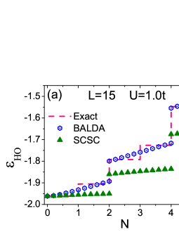
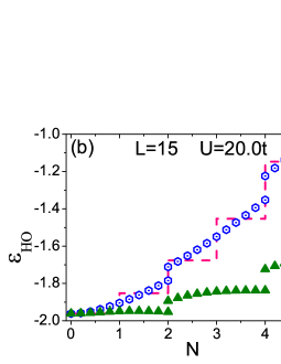
Figure 2: (Color online) Open Hubbard chains of $L=15$ sites: HO KS eigenvalues ($\varepsilon_{\textrm{HO}}$) for $0<N\leq 5$.

3.1.1 Spin-orbital separation

The difficulty with energy gaps is intrinsic of most available density functionals. In this context, beyond spinons and chargons, we propose here a model for the third electron fractionalization: into orbitons. By definition, orbitons are excitations of the orbital degrees of freedom of electrons, which behave like spinless and uncharged particles. As consequence, when dealing with the noninteracting KS electrons of fig. 1 (c), we propose the KS eigenvalues should be increased by a constant $\Delta$, which is equivalent to include the presence of an “anti-orbiton”, the extension of the SCSC idea of eq. 11. Thus, we propose the XC potential to be given by

$$v_{xc}^{approx+\Delta}[n](j)=v_{xc}^{approx}[n](j)+\Delta,$$ (13)

with

$$\Delta=\varepsilon_{(\textrm{HO}+\eta)}-\varepsilon_{\textrm{HO}};\ \ \ \eta=0,1,2,...$$ (14)

As conceptually thought, the parameter $\eta$ is given by:

$$\eta=\frac{N_{\textrm{even}}}{2},$$ (15)

for

$$N_{\textrm{even}}-1<N\leq N_{\textrm{even}}+1.$$ (16)

For example, in the strongly interacting limit, $\eta=1$ for $1<N\leq 3$ and $\eta=2$ for $3<N\leq 5$. Noninteracting systems (or interacting systems with $0<N\leq 1$) should have $\eta=0$, indicating the absence of spin-orbital separation. A schematic representation of this orbital separation model is shown in fig. 3.

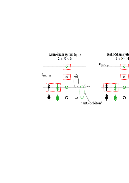
Figure 3: (Color online) Noninteracting Kohn-Sham systems: Spins and charges together, at expense of the presence of spinless holons and the conjectured “anti-orbitons”. The anti-orbitons are represented by excitations between orbital levels.

Let us define $\varepsilon_{\textrm{HO}}^{\Delta}$ as the HO KS eigenvalues yielded by the $v_{xc}^{approx+\Delta}$ potential. By means of eqs. 13 and 14, $\varepsilon_{\textrm{HO}}^{\Delta}$ can be determined by means of the following KS equation:

$$\begin{split}\left\{\hat{t}_{s}\right.+&v_{ext}(j)+v_{H}[n](j)\left.+v_{xc}^{approx}[n](j)\right\}\psi_{i\sigma}(j)=\varepsilon_{i\sigma}\ \psi_{i\sigma}(j),\end{split}$$ (17)

with

$$\varepsilon_{\textrm{HO}}^{\Delta}=\varepsilon_{(\textrm{HO}+\eta)}.$$ (18)

The orbital degrees of freedom we mention here come from the solution of the Hubbard-like KS equations, under the Hubbard Hamiltonian of eq. 12, and does not come from a multi-band Hubbard model.

In fig. 4 (a)-(d) we plot the results for the BALDA$+\Delta$ and SCSC$+\Delta$. The inclusion of $\Delta$ yields $E_{g}\neq 0$ for open and closed shells. At strong correlations (when $U$ is increased), the curves of SCSC$+\Delta$ fit in very good agreement with the exact data, including the constancy of $\varepsilon_{\textrm{HO}}$, the derivative discontinuities of the XC potentials and the ionization potentials. The BALDA$+\Delta$ also yields correct energy gaps, but combined with incorrect IPs and linear dependence of $\varepsilon_{\textrm{HO}}$ between integers.

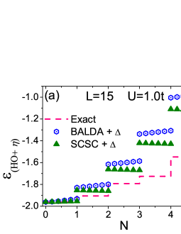
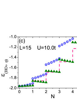
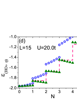
Figure 4: (Color online) Open Hubbard chains of $L=15$ sites: HO KS eigenvalues ($\varepsilon_{\textrm{HO}}$) obtained by including the $\Delta$ factor of eqs. 13 and 14, with $\eta$ given by eqs. 15 and 16.

3.2 One-dimensional H₂ molecule in the continuum

In dissociation processes, to preserve neutrality of isolated atoms, it is known that the increment of nuclear separation uses to be followed by an increment of correlation energy density.⁹ In order to test the spinon-chargon-orbiton approach under this type of delimitation weakly-strongly correlated systems, in this section we consider the dissociation of a 1D H₂ molecule.

In contrast with the discrete Hubbard chains, a different way of describing interacting electrons in one-dimension may take into account (a) continuum space and (b) long-ranged Coulomb interaction. This is a special case of interest, since chemistry in general is described by using both ingredients. The electronic Hamiltonian of a 1D H₂ molecule can be written as:

$$\hat{H}=\sum_{j=1}^{2}\left[-\frac{1}{2}\frac{d^{2}}{dx_{j}^{2}}+v_{\textrm{ext}}(x_{j})\right]+\frac{1}{2}\sum_{j,k=1\atop(j\not=k)}^{2}v_{\textrm{int}}(x_{j},x_{k}).$$ (19)

A common choice, which avoids singularities of the Coulomb interaction, is the soft-Coulomb potential:^{35, 36, 37, 38}

$$v_{\textrm{int}}(x_{j},x_{k})=\frac{q_{j}q_{k}}{\sqrt{b^{2}+(x_{j}-x_{k})^{2}}},$$ (20)

where $q_{j}$ and $q_{k}$ are the electron charges placed at positions $x_{j}$ and $x_{k}$, respectively, and $b$ is a softening parameter. The same idea holds for the electron-nucleus interactions:

$$v_{\textrm{ext}}(x_{j})=\sum_{i=1}^{2}\frac{Z_{i}\leavevmode\nobreak\ q_{j}}{\sqrt{b^{2}+\left(x_{j}-X_{i}\right)^{2}}},$$ (21)

labelling the nuclear charge $Z_{i}$ placed at position $X_{i}$. The repulsive nucleus-nucleus interaction (not showed) is also described by means of a soft-Coulomb potential (under the same parameter $b$). Specifically for $b=1$, a local-density approximation (1DLDA) has been used to describe one-dimensional atoms and molecules.^{36, 37, 38} Here we intend to use the 1DLDA and implement the corresponding SCSC$+\Delta$ correction to it. In this section, we shall denote the SCSC/1DLDA approach simply as SCSC approximation.

In fig. 5 (a), considering $0<N\leq 2$, we plot $\varepsilon_{\textrm{HO}}$ for a 1D H₂ molecule with nuclear separation $d=X_{2}-X_{1}=1.6$ a.u., which is the exact equilibrium distance.³⁷ The values of $\varepsilon_{\textrm{HO}}$ follow the same trend as observed in the previous figures, displaying typical errors of weakly correlated situations. As the separation $d$ is increased, on the other hand, the SCSC$+\Delta$ yields very accurate data for $\varepsilon_{\textrm{HO}}$, as seen from fig. 5 (b), valid for $d=4.0$ a.u.: It is a clear delimitation between weakly and strongly correlated systems, under a fixed value of $b$. These results are in accordance with the observation that correlation energy density is zero in isolated H atoms but substantial around each H atom in H₂ at long distances.^{39, 40}

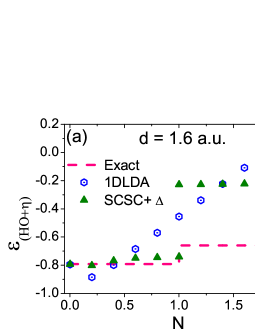
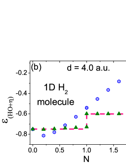
Figure 5: (Color online) One-dimensional H₂ molecule in the continuum. (a) HO KS eigenvalues ($\varepsilon_{\textrm{HO}}$) for $0<N\leq 2$ and nuclear separation $d=1.6$ a.u. (b) The same as before, but for $d=4.0$ a.u. Remember: for 1DLDA, $\eta=0$ for $0<N\leq 2$; in the case of SCSC$+\Delta$, $\eta=0$ for $0<N\leq 1$ and $\eta=1$ for $1<N\leq 2$. The “exact” data come from total energies, directly extracted from the literature.³⁷

In summary, we can conclude that: (l) spin-charge separation, when included by means of the SCSC XC potential, yields almost constant highest occupied KS eigenvalues; (ll) in the limits of strong correlations, the model we proposed here for the spin-orbital separation yields accurate energy gaps for both, open and closed shells (in association with correct derivative discontinuities of the XC potentials). Considering (l) and (ll), we can argue that when dealing with strong correlations, electrons should not be treated as unique particles. Instead, the separation into spinons, chargons and orbitons can be crucial. The way to include it in a noninteracting KS calculation, which by construction retains spin, charge and orbital degrees of freedom together, is a combination of (l) and (ll).

4 Conclusions

Constancy of $\varepsilon_{\textrm{HO}}$: The BALDA-FN and 1DLDA yielded typical results attributed to delocalization errors of density functionals: Incorrect linear behavior of $\varepsilon_{\textrm{HO}}$ upon fractional charge occupation. On the other hand, the SCSC/BALDA-FN and SCSC/1DLDA, which have been especially conceived to deal with strong correlations, yielded almost constant values for $\varepsilon_{\textrm{HO}}$.

Derivative discontinuity: By means of eq. 13, we proposed the inclusion of the extra electron fractionalization – into orbitons – which yielded accurate energy gaps at strong correlations. We observed a delimitation between weak and strong correlations by simply changing the on-site interaction $U$, in open Hubbard chains, or changing the nuclear separation (at fixed interaction parameter $b$) in the dissociation of a 1D H₂ molecule. It has been recently pointed out that, beyond strong correlations, it is a basic challenge to understand whether the KS orbitals and eigenvalues have any further significance.⁹ The spinon-chargon-orbiton separation can therefore be a step into this direction.

Energy functionals: Testing the SCSC and SCSC$+\Delta$ potentials under different paths of assigning energy functionals^{25, 26} is a topic of future investigation. The resulting energy functionals may then be used in the derivation of even more accurate XC potentials, which, for example, could suitably link the weakly and strongly correlated regimes.

Extensions: Possible direct generalizations to higher dimensions, especially to three-dimensional (3D) systems, depend on a particular question: Is electron fractionalization also possible in 3D? At our knowledge, this is still a topic of debate, and therefore deserves further investigation. Nevertheless, indirect generalizations are certainly possible, as the case of quasi one-dimensional systems.

It should be noted that a successful alternative route to obtain accurate derivative discontinuities and constancy of $\varepsilon_{\textrm{HO}}$ – the SCE approach – has been described in recent letters.^{41, 42} In this sense, understanding possible connections between using SCSC+$\Delta$ and other accurate approaches is also a topic of future investigation.

Acknowledgments: We thank Vivaldo L. Campo Jr. for his code of Lanczos exact diagonalization and for the original version of the BALDA-FN code.

References

- 1
- 2 T. Giamarchi, Quantum Physics in One Dimension (Oxford University Press, Oxford, 2003).
- 3 Wohlfeld, K.; Daghofer, M.; Nishimoto, S.; Khaliullin, G.; van den Brink, J. Phys. Rev. Lett. 2011, 107, 147201.
- 4 Schlappa, J.; Wohlfeld, K.; Zhou, K. J.; Mourigal, M.; Haverkort, M. W.; Strocov, V. N.; Hozoi, L.; Monney, C.; Nishimoto, S.; Singh, S.; Revcolevschi, A.; Caux, J.-S.; Patthey, L.; R nnow, H. M.; van den Brink, J.; Schmitt, T. Nature 2012, 485, 82.
- 5 Jompol, Y.; Ford, C. J. B.; Griffiths, J. P.; Farrer, I.; Jones, G. A. C.; Anderson, D.; Ritchie, D. A.; Silk, T. W.; Schofield, A. J. Science 2009, 325, 597.
- 6 Kohn, W. Rev. Mod. Phys. 1999, 71, 1253.
- 7 Capelle, K. Braz. J. Phys. 2006, 36, 1318.
- 8 Vieira, D. Phys. Rev. B 2012, 86, 075132.
- 9 Cohen, A. J.; Mori-Sánchez, P.; Yang, W. Chem. Rev. 2012, 112, 289.
- 10 Ruzsinszky, A.; Perdew, J. P.; Csonka, G. I.; Vydrov, O. A.; Scuseria, G. E. J. Chem. Phys. 2006, 125, 194112.
- 11 Kümmel, S.; Kronik, L. Rev. Mod. Phys. 2008, 80, 3.
- 12 Cohen, A. J.; Mori-Sánchez, P.; Yang, W. Science 2008, 321, 792.
- 13 Mori-Sánchez, P.; Cohen, A. J.; Yang, W. Phys. Rev. Lett. 2008, 100, 146401.
- 14 Perdew, J. P.; Parr, R. G.; Levy, M.; Balduz Jr., J. L. Phys. Rev. Lett. 1982, 49, 1691.
- 15 Janak, J. Phys. Rev. B 1978, 18, 7165.
- 16 Capelle, K.; Vignale, G.; Ullrich, C. A. Phys. Rev. B 2010, 81, 125114.
- 17 Voit, J. Rep. Prog. Phys. 1995, 58, 977.
- 18 Miranda, E. Braz. J. Phys. 2003, 33, 3.
- 19 A. Khare, Fractional Statistics and Quantum Theory (World Scientific Publishing, 2005).
- 20 Bernevig, B.A.; Giuliano, D.; Laughlin, R. B. Phys. Rev. Lett. 2001, 87, 177206.
- 21 For example, consider a two-electron system of opposite spins. In the limit of strong electron-electron interaction, the situation is equivalent to a system of noninteracting spinless electrons, which singly occupy the two lowest quantum states (in the ground-state).
- 22 Karolewski, A.; Armiento, R.; Kümmel, S. J. Chem. Theory Comput. 2009, 5, 712.
- 23 Oliveira, M. J. T.; Räsänen, E.; Pittalis, S.; Marques, M. A. L. J. Chem. Theory Comput. 2010, 6, 3664.
- 24 Boguslawski, K.; Jacob, C. R.; Reiher, M. J. Chem. Phys. 2013, 138, 044111.
- 25 Gaiduk, A. P.; Staroverov, V. N. J. Chem. Phys. 2012, 136, 064116.
- 26 Elkind, P. D.; Staroverov, V. N. J. Chem. Phys. 2012, 136, 124115.
- 27 Hubbard, J. Proc. Roy. Soc. (London) A 1963, 276, 238.
- 28 For this reason, in spite of using the XC nomenclature, we shall deal only with correlation.
- 29 Schönhammer, K.; Gunnarsson, O.; Noack, R. M. Phys. Rev. B 1995, 52, 2504.
- 30 Lima, N. A.; Silva, M. F.; Oliveira, L. N.; Capelle, K. Phys. Rev. Lett. 2003, 90, 146402.
- 31 França, V. V.; Vieira, D.; Capelle, K. New J. Phys. 2012, 14, 073021.
- 32 Xianlong, G.; Polini, M.; Tosi, M. P.; Campo, V. L.; Capelle, K.; Rigol, M. Phys. Rev. B 2006, 73, 165120.
- 33 Capelle, K.; Campo, V. L. Phys. Rep. 2013, 528, 91.
- 34 Xianlong, G.; Chen, A-H.; Tokatly, I. V.; Kurth, S. Phys. Rev. B 2012, 86, 235139.
- 35 Tempel, D. G.; Martínez, T. J.; Maitra, N. T. J. Chem. Theory Comput. 2009, 5, 770.
- 36 Helbig, N.; Fuks, J. I.; Casula, M.; Verstraete, M. J.; Marques, M. A. L.; Tokatly, I. V.; Rubio, A. Phys. Rev. A 2011, 83, 032503.
- 37 Wagner, L. O.; Stoudenmire, E. M.; Burke, K.; White, S. R. Phys. Chem. Chem. Phys. 2012, 14, 8581.
- 38 Stoudenmire, E. M.; Wagner, L. O.; White, S. R.; Burke, K. Phys. Rev. Lett. 2012, 109, 056402.
- 39 Süle, P.; Gritsenko, O. V.; Nagy, A.; Baerends, E. J. J. Chem. Phys. 1995, 103, 10085.
- 40 Baerends, E. J. Phys. Rev. Lett. 2001, 87, 133004.
- 41 Malet, F.; Gori-Giorgi, P. Phys. Rev. Lett. 2012, 109, 246402.
- 42 Mirtschink, A.; Seidl, M.; Gori-Giorgi, P. Phys. Rev. Lett. 2013, 111, 126402.