Kaon semileptonic decays near the physical point

Abstract:

The CKM matrix element $|V_{us}|$ can be extracted from the experimental measurement of semileptonic $K\to\pi$ decays. The determination depends on theory input for the corresponding vector form factor in QCD. We present a preliminary update on our efforts to compute it in $N_{f}=2+1$ lattice QCD using domain wall fermions for several lattice spacings and with a lightest pion mass of about $170\,\mathrm{MeV}$. By using partially twisted boundary conditions we avoid systematic errors associated with an interpolation of the form factor in momentum-transfer, while simulated pion masses near the physical point reduce the systematic error due to the chiral extrapolation.

1 Introduction

In the Standard Model (SM) the unitary Cabibbo-Kobayashi-Maskawa (CKM) matrix contains information on the strength of flavour-changing weak decays as well as information on correlations between different such processes. Inconsistencies in the CKM-picture would indicate the presence of new physics beyond the SM. One therefore tries to determine all CKM-matrix elements as precisely as possible by studying flavour changing processes both experimentally (e.g. at NA62 and LHCb at CERN) and theoretically. Here we concentrate on the determination of the matrix element $|V_{us}|$ from the study of semileptonic kaon ($K_{l3}$) decays which enables a test of first-row CKM-unitarity, $|V_{ud}|^{2}+|V_{us}|^{2}+|V_{ub}|^{2}=1$. $|V_{ub}|$ is neglected because it is smaller than the errors in the other two terms on the l.h.s., $|V_{us}|$ and $|V_{ud}|$. $|V_{ud}|$ is known very precisely from neutron $\beta$-decay and matching the corresponding precision for $|V_{us}|$ is crucial in searching for deviations from CKM-unitarity and for possible signs of new physics.

In this talk we present an update on our precision-study of the $K_{l3}$ form factor, $f_{+}(0)$ [1, 2]. The novelties are simulations at lighter quark masses corresponding to a lightest pion mass of about $170\,\mathrm{MeV}$ [3] and two additional lattice spacings. Both allow for considerably improved control over systematic effects.

2 Kaon semileptonic decays

To date, one of the most precise determinations of $|V_{us}|$ comes from $K\to\pi l\nu$ semileptonic decays (cf. [4]): The product $|V_{us}|^{2}|f_{+}(0)|^{2}$ can be determined with a precision at the per mil level from the experimental decay rate [5] and lattice QCD provides the value for $f_{+}(0)$. Currently the level of precision set by experiment sets the precision goal for lattice simulations.

The form factor $f_{+}(0)$ is defined from the vector part of the strangeness-changing weak current ($V_{\mu}=\bar{s}\gamma_{\mu}u$) according to

$$\langle\pi(p^{\prime})\big{|}V_{\mu}\big{|}K(p)\rangle=(p_{\mu}+p_{\mu}^{\prime})f_{+}(q^{2})+(p_{\mu}-p_{\mu}^{\prime})f_{-}(q^{2})\,,$$ (1)

where $q^{2}=(p-p^{\prime})^{2}$ is the momentum transfer. We define the scalar form factor

$$f_{0}(q^{2})=f_{+}(q^{2})+\frac{q^{2}}{m_{K}^{2}-m_{\pi}^{2}}f_{-}(q^{2})\,,$$ (2)

with $f_{0}(0)=f_{+}(0)$. In the SU(3) flavour limit where $m_{K}^{2}=m_{\pi}^{2}$, $f_{+}(0)\nolinebreak=\nolinebreak 1$ by vector current conservation. It can be expanded in terms of the meson masses as $f_{+}(0)=1+f_{2}+\ldots$ where $f_{n}=O(m_{\pi}^{n},m_{K}^{n},m_{\eta}^{n})$ [6]. $f_{2}$ is a known function of meson masses and the SU(3) pseudoscalar decay constant. In lattice simulations therefore effectively only the small higher order correction $\Delta f=f_{+}(0)-(1+f_{2})$ is computed and extrapolated to the physical point.

We compute the matrix element in (1) in terms of the ground-state contribution to suitable ratios of Euclidean two- and three-point functions. In a finite lattice box with periodic boundary conditions for the quark fields, the matrix element can in this way only be computed for meson momenta corresponding to the Fourier modes, i.e. $\frac{2\pi}{L}\vec{n}$ with $n_{i}=\pm 0,\pm 1,\dots$ for a spatial volume $V=L^{3}$. The form factor at $q^{2}=0$ is then computed by interpolating between the data for the form factor at these Fourier-points [1] thereby introducing a dependence of the final result on the interpolation model; different ansätze may lead to different results for the form factor, introducing systematic uncertanities.

3 Partially twisted boundary condition

In contrast to periodic boundary conditions, twisted boundary conditions allow access to hadron momenta other than $\frac{2\pi}{L}\vec{n}$ [8]. Here we employ partially twisted boundary conditions [9] by applying the twist only to the valence quarks,

$$q(x_{i}+L)=e^{i\,\theta_{i}}q(x_{i})\,,$$ (3)

($\theta_{i}$ is the twist angle in the $\hat{i}$-direction). In our simulation a charged meson of mass $m$ with one of the valence quarks twisted with angle $\vec{\theta}$ then obeys the dispersion relation

$$E=\sqrt{m^{2}+\left(\frac{2\pi}{L}\vec{n}+{\vec{\theta}}/{L}\right)^{2}},$$ (4)

up to exponentially supressed finite volume corrections [9]. For matrix elements like $K\to\pi$, where the initial and final state mesons carry twists $\vec{\theta}_{i}$ and $\vec{\theta}_{f}$, respectively, the momentum transfer can be written as [10]

$$q^{2}=(p_{i}-p_{f})^{2}=\Big{[}E_{i}(\vec{p}_{i})-E_{f}(\vec{p}_{f})\Big{]}^{2}-\left[\left(\frac{2\pi}{L}\vec{n}_{i}+\frac{\vec{\theta_{i}}}{L}\right)-\left(\frac{2\pi}{L}\vec{n}_{f}+\frac{\vec{\theta_{f}}}{L}\right)\right]^{2}\,.$$ (5)

By adjusting the twists on the initial and final meson (here $K,\pi$), we can evaluate $f_{+}$ directly at $q^{2}=0$. The commonly used implementation is to contruct ratios of correlation functions, $R_{K\pi}(\vec{p}_{K},\vec{p}_{\pi})$ (see e.g. [10]), where either the kaon or pion is kept at rest and where the twist on the other meson is tuned in order to obtain results [10]:

$$\begin{array}[]{llcccc}&R_{K\pi}(\vec{p}_{K},\vec{0})&\textrm{with}&|\vec{\theta}_{K}|=L\sqrt{\left({m_{K}^{2}+m_{\pi}^{2}\over 2m_{\pi}}\right)^{2}-m_{K}^{2}}&\textrm{and}&\vec{\theta}_{\pi}=\vec{0}\,,\\ {\rm and}&R_{K\pi}(\vec{0},\vec{p}_{\pi})&\textrm{with}&|\vec{\theta}_{\pi}|=L\sqrt{\left({m_{K}^{2}+m_{\pi}^{2}\over 2m_{K}}\right)^{2}-m_{\pi}^{2}}&\textrm{and}&\vec{\theta}_{K}=\vec{0}\,.\\ \end{array}$$ (6)

The form factor $f_{0}(0)$ can then be evaluated directly at $q^{2}=0$ as

$$f_{0}(0)=\frac{R_{K\pi}(\vec{p}_{K},\vec{0})(m_{K}-E_{\pi})-R_{K\pi}(\vec{0},\vec{p}_{\pi})(E_{K}-m_{\pi})}{(E_{K}+m_{\pi})(m_{K}-E_{\pi})-(m_{K}+E_{\pi})(E_{K}-m_{\pi})}\,.$$ (7)

This expression is derived by considering only the time-component of the vector current matrix element (1). Using all the other components of the weak vector current, we can construct an over-constrained system of equations

$$R_{K\pi}(\vec{\theta}_{K},\vec{0},V_{t}) = f_{+}(0)\,(E_{K}+m_{\pi})+f_{-}(0)\,(E_{K}-m_{\pi})\,,$$

$$R_{K\pi}(\vec{0},\vec{\theta}_{\pi},V_{t}) = f_{+}(0)\,(m_{K}+E_{\pi})+f_{-}(0)\,(m_{K}-E_{\pi})\,,$$

$$R_{K\pi}(\vec{\theta}_{K},\vec{0},V_{i}) = f_{+}(0)\,\theta_{K,i}+f_{-}(0)\,\theta_{K,i}\,,$$

$$R_{K\pi}(\vec{0},\vec{\theta}_{\pi},V_{i}) = f_{+}(0)\,\theta_{\pi,i}-f_{-}(0)\,\theta_{\pi,i}\ ,\qquad(i=x,y,z)\,,$$ (8)

which we solve to obtain the form factors directly at $q^{2}=0$. Note that distributing the twist over all spatial directions maximises the number of non-trivial equations. Having eliminated the systematic error due to the $q^{2}$ interpolation, the remaining dominant source of systematic uncertainty is due to the chiral extrapolation of the lattice data to the physical point [2].

4 Results

In [1] we presented results for the form factor from simulations of domain wall fermions (DWF) with the Iwasaki Gauge action, an inverse lattice spacing of 1.7GeV and $m_{\pi}$ in the range $330$–$700\,\mathrm{MeV}$. Here we extend the analysis by adding new ensembles 32Fine [11], 32Coarse [12] (cf. table 1) providing data for considerably lighter pion masses down to $170\,\mathrm{MeV}$ and two additional lattice spacings.

Label	Size	$S_{G}$	$a^{-1}$	$m_{\pi}(\,\mathrm{MeV})$
24Coarse	$24^{3}\times 64\times 16$	Iwasaki	1.75(4)	$330$, $420$, $550$ , $670$
32Fine	$32^{3}\times 64\times 16$	Iwasaki	2.31(4)	$290$, $350$, $400$
32Coarse	$32^{3}\times 64\times 32$	Iwasaki+DSDR	1.37(1)	$170$, $250$

Table 1: A summary of the three ensembles used in this analysis. Here ‘$S_{G}$’ denotes the Gauge action, ‘$m_{\pi}$’ the pion mass and $a^{-1}$ the lattice spacing. The 32Fine and 32Coarse data are new in this calculation.

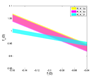
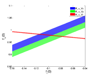
Figure 1: Plot of $f_{+}(0)$ vs. $f_{-}(0)$ for kaon(left) and pion(right) only twisted equations

Closer to the physical point the twist-angles prescribed by eqs. (6) are very large, in particular for the case where the kaon is moving and the pion is at rest. This manifests itself in larger statistical fluctuations for the ratio $R_{K\pi}(\vec{p}_{K},\vec{0})$. In order to find a better choice of kinematics we analysed the situation further: From eq. (3), the slope of $f_{+}(0)$ with respect to $f_{-}(0)$ is given by

$$\frac{\partial f_{+}(0)}{\partial f_{-}(0)}\bigg{|}_{\theta_{K}=0}=-\frac{m_{K}-E_{\pi}}{m_{K}+E_{\pi}}\,,\qquad\frac{\partial f_{+}(0)}{\partial f_{-}(0)}\bigg{|}_{\theta_{\pi}=0}=-\frac{E_{K}-m_{\pi}}{E_{K}+m_{\pi}}\,,$$ (9)

for the matrix element of the time-component of the vector current, $V_{t}$, and

$$\frac{\partial f_{+}(0)}{\partial f_{-}(0)}\bigg{|}_{\theta_{K}=0}=1\qquad\frac{\partial f_{+}(0)}{\partial f_{-}(0)}\bigg{|}_{\theta_{\pi}=0}=-1\,,$$ (10)

for the spatial components $V_{x,y,z}$.

Figure 2: Plot of $f_{+}(0)$ vs. $f_{-}(0)$ for the cases where (left) both pion and kaon are twisted (right) pion only and kaon only twisted equations are combined.

The solutions for all equations for ($\vec{p}_{K},\vec{0}$) and ($\vec{0},\vec{p}_{\pi}$) on the 32Coarse ensemble with $m_{\pi}=250\,\mathrm{MeV}$ are shown in the l.h.s. and r.h.s. plots in Fig 1, respectively. While all solutions have a negative slope for the case where only the kaon is twisted, there are solutions with opposite slopes in the case where the pion is twisted. Because the solution is given by the intersection of the individual constraints, the kinematical situation where the pion is moving (twisted) and the kaon is at rest provides the best result. The statistical errors are also smaller in this case. Motivated by these observations, we computed all correlation functions once again for a third choice of kinematics with $q^{2}=0$, where both the kaon and the pion are twisted. This leads to a good constraint for $f_{+}(0)$ as shown in the left plot in Fig. 2. The result is in agreement with the result obtained by solving all simultaneous equations for the cases where either the pion or the kaon are twisted as shown in the right plot of Fig. 2 (obtained by combining the plots in Fig. 1).

We now turn our attention to the mass- and momentum-dependence of the results. In principle, using partially twisted boundary conditions, one is independent of the momentum interpolation. We wish however to include our earlier data sets, the three heavier ensembles in the 24Coarse set, for which we have not generated data directly at $q^{2}=0$. From [1] we know that in these cases the interpolation introduces hardly any model-dependence. In addition to the momentum-dependence a fit ansatz should also incorporate the $\mathrm{SU}(3)$-symmetry-breaking nature of $f_{+}(0)$ and the strange quark mass dependence since the simulated strange quark mass is not exactly at the physical point. Our ansatz with four fit parameters $A_{0},A_{1},M_{0},M_{1}$ [1] is

$$f_{0}(q^{2},m_{\pi}^{2},m_{K}^{2})=\frac{1+f_{2}+(m_{K}^{2}-m_{\pi}^{2})^{2}(A_{0}+A_{1}(m_{K}^{2}+m_{\pi}^{2}))}{1-q^{2}/(M_{0}+M_{1}(m_{K}^{2}+m_{\pi}^{2}))^{2}}\,.$$ (11)

$\begin{array}[]{cc}\includegraphics[scale={0.42}]{images/mpi_dependence_32}&\includegraphics[scale={0.42}]{images/mpi_dependence_32corr}\end{array}$

Figure 3: Plot of $f_{+}(0)$ dependence on $m_{\pi}^{2}$. Left : raw data points at the simulated (uncorrected) strange quark masses. Right : The data points are shifted to physical strange quark mass. In both plots, the curve uses a parameterisation for the kaon mass with strange quark held fixed at its physical value.

Fig 3 (left) summarizes the results of the analysis for all ensembles. The data points are the ones for the simulated, i.e. unphysical strange-quark mass. After correcting towards the physical strange-quark mass using the ansatz in eq. (11), all data points line up on the fit-curve in the r.h.s. plot in Fig. 3. Our preliminary result for $f_{+}(0)$ at the physical point is indicated by the light blue square. At this early stage of the analysis we find that the statistical error at the physical point has been reduced with respect to our earlier results [2].

In our fit ansatz we use the decay constant in the chiral limit, $f_{0}$, in the NLO term and have a form for the NNLO term which together make the ansatz consistent with the Ademollo-Gatto theorem and symmetry under interchange of $m_{\pi}$ and $m_{K}$. Since we do not know the precise value for $f_{0}$, we repeat the global fit for $f_{0}=100,115$ and $131\,\mathrm{MeV}$. This variation in $f_{0}$ is also assumed to account partially for our NNLO term not being the full chiral perturbation theory expression. The result for $f_{+}(0)$ using $f_{0}=115\,\mathrm{MeV}$ is taken as our best value and the values at $100$ and $131\,\mathrm{MeV}$ provide an estimate of the systematic error from the chiral extrapolation.

Figure 4: Comparison of recent Lattice results

In Fig. 4 we compare our new preliminary result for $f_{+}(0)$ with other recent Lattice determinations. We emphasize that our result is preliminary, but we expect to reach a new level of precision when the analysis is complete.

5 Conclusion

We have presented an update on our simulations aiming at the precise prediction of the kaon semileptonic form factor at vanishing momentum transfer. The novelties are simulations for pion masses down to $170\,\mathrm{MeV}$ and for three different lattice spacings. We identified preferred choices for the kinematics when using partially twisted boundary conditions in order to simulate directly at $q^{2}=0$. In particular, we now understand why twisting either only the pion or both the kaon and the pion can constrain the form factor better than twisting only the kaon. At this early stage of the analysis the inclusion of the new ensembles in our global fit leads to a reduction of the statistical error at the physcial point compared to our earlier result [2]. This indicates significant progress in the study of K $\to$ $\pi$ semileptonic form factors which would directly impact our knowledge of the CKM Matrix and provide for improved constraints for new physics beyond the Standard Model.

6 Acknowledgement

We thank our colleagues in RBC and UKQCD within whose programme this calculation was performed. The computations were done using the STFC’s DiRAC facility at Swansea, JUGENE at the Jülich Supercomputing Centre and the DiRAC facility at Edinburgh. KS acknowledges support by the European Union under the Grant Agreement number 238353 (ITN STRONGnet); CTS and JMF by STFC grant ST/J000396/1 and ST/H008888/1; P.A.B, by STFC grants ST/K000411/1, ST/J000329/1 and ST/H008845/1; AJ by European Research Council (FP7/2007-2013)/Grant agreement 27975; and JMZ by the Australian Research Council under grant FT100100005.

References

- [1] P. A. Boyle et al. [RBC/UKQCD], Phys. Rev. Lett. 100 (2008) 141601, [arXiv:0710.5136].
- [2] P. A. Boyle et al. [RBC/UKQCD], Eur. Phys. J. C 69 (2010) 159 [arXiv:1004.0886 [hep-lat]].
- [3] R. Arthur et al. [RBC/UKQCD], arXiv:1208.4412 [hep-lat].
- [4] G. Colangelo et al. [FLAG], Eur.Phys.J. C71 1695 (2011).
- [5] M. Antonelli et al., Eur.Phys.J. C69 399-424 (2010).
- [6] J. Gasser and H. Leutwyler, Nucl. Phys. B250 (1985) 517-538.
- [7] H. Leutwyler and M. Roos, Z. Phys. C 25, 91 (1984).
- [8] P. F. Bedaque and J.-W. Chen, Phys. Lett. B616 (2005) 208–214, [hep-lat/0412023].
- [9] C. T. Sachrajda and G. Villadoro, Phys. Lett. B609 (2005) 73–85, [hep-lat/0411033].
- [10] P. A. Boyle et al. [RBC/UKQCD], JHEP 05 (2007) 016, [hep-lat/0703005].
- [11] Y. Aoki et al. [RBC/UKQCD], Phys. Rev. D83 (2001) 074508.
- [12] R. Arthur et al. [RBC/UKQCD], arXiv:1208.4412.
- [13] M. Ademollo and R. Gatto, Phys. Rev. Lett. 13, 264 (1964).