Information Capacity of an Energy Harvesting Sensor Node

Abstract

Energy harvesting sensor nodes are gaining popularity due to their ability to improve the network life time and are becoming a preferred choice supporting “green communication”. In this paper we focus on communicating reliably over an AWGN channel using such an energy harvesting sensor node. An important part of this work involves appropriate modeling of the energy harvesting, as done via various practical architectures. Our main result is the characterization of the Shannon capacity of the communication system. The key technical challenge involves dealing with the dynamic (and stochastic) nature of the (quadratic) cost of the input to the channel. As a corollary, we find close connections between the capacity achieving energy management policies and the queueing theoretic throughput optimal policies.

Keywords: Information capacity, energy harvesting, sensor networks, fading channel, energy buffer, network life time.

I Introduction

Sensor nodes are often deployed for monitoring a random field. These nodes are characterized by limited battery power, computational resources and storage space. Once deployed, the battery of these nodes are often not changed because of the inaccessibility of these nodes. Nodes could possibly use larger batteries but with increased weight, volume and cost. Hence when the battery of a node is exhausted, it is not replaced and the node dies. When sufficient number of nodes die, the network may not be able to perform its designated task. Thus the life time of a network is an important characteristic of a sensor network ([1]) and it depends on the life time of a node.

The network life time can be improved by reducing the energy intensive tasks, e.g., reducing the number of bits to transmit ([2], [3]), making a node to go into power saving modes (sleep/listen) periodically ([4]), using energy efficient routing ([5], [6]), adaptive sensing rates and multiple access channel ([7]). Network life time can also be increased by suitable architectural choices like the tiered system ([8]) and redundant placement of nodes ([9]).

Recently new techniques of increasing network life time by increasing the life time of the battery is gaining popularity. This is made possible by energy harvesting techniques ([10], [11]). Energy harvestesr harness energy from the environment or other energy sources ( e.g., body heat) and convert them to electrical energy. Common energy harvesting devices are solar cells, wind turbines and piezo-electric cells, which extract energy from the environment. Among these, harvesting solar energy through photo-voltaic effect seems to have emerged as a technology of choice for many sensor nodes ([11], [12]). Unlike for a battery operated sensor node, now there is potentially an infinite amount of energy available to the node. However, the source of energy and the energy harvesting device may be such that the energy cannot be generated at all times (e.g., a solar cell). Furthermore the rate of generation of energy can be limited. Thus one may want to match the energy generation profile of the harvesting source with the energy consumption profile of the sensor node. If the energy can be stored in the sensor node then this matching can be considerably simplified. But the energy storage device may have limited capacity. The energy consumption policy should be designed in such a way that the node can perform satisfactorily for a long time, i.e., energy starvation at least, should not be the reason for the node to die. In [10] such an energy/power management scheme is called energy neutral operation.

In the following we survey the relevant literature. Early papers on energy harvesting in sensor networks are [13] and [14]. A practical solar energy harvesting sensor node prototype is described in [15]. In [10] various deterministic models for energy generation and energy consumption profiles are studied and provides conditions for energy neutral operation. In [16] a sensor node is considered which is sensing certain interesting events. The authors study optimal sleep-wake cycles such that event detection probability is maximized. A recent survey on energy harvesting is [17].

Energy harvesting can be often divided into two major architectures ([15]). In Harvest-use(HU), the harvesting system directly powers the sensor node and when sufficient energy is not available the node is disabled. In Harvest-Store-Use (HSU) there is a storage device that stores the harvested energy and also powers the sensor node. The storage can be single or double staged ([10], [15]).

Various throughput and delay optimal energy management policies for energy harvesting sensor nodes are provided in [18]. The energy management policies in [18] are extended in various directions in [19] and [20]. For example, [19] also provides some efficient MAC policies for energy harvesting nodes. In [20] optimal sleep-wake policies are obtained for such nodes. Furthermore, [21] considers jointly optimal routing, scheduling and power control policies for networks of energy harvesting nodes. Energy management policies for finite data and energy buffer are provided in [22]. Reference [23] provides optimal energy management policies and energy allocation over source acquisition/compression and transmission.

In a recent contribution, optimal energy allocation policies over a finite horizon and fading channels are studied in [24]. Relevant literature for models combining information theory and queuing theory are [25] and [26].

The capacity of a fading Gaussian channel with channel state information (CSI) at the transmitter and receiver and at the receiver alone are provided in [27]. It was shown that optimal power adaptation when CSI is available both at the transmitter and the receiver is ‘water filling’ in time.

Information-theoretic capacity of an energy harvesting system has been considered previously in [28] and [29] independently. It was shown that the capacity of the energy harvesting AWGN channel with an unlimited battery is equal to the capacity with an average power constraint equal to average recharge rate. In [29] the proof technique used is based on AMS sequences [30] which is different from that used in [28].

Our main contributions are in considering significant extensions to the basic energy harvesting system by considering processor energy, energy inefficiencies (and finally channel fading). We compute the capacity when the energy is consumed in other activities at the node (e.g., processing, sensing, etc) than transmission. This issue of energy consumed in processing in the context of the usual AWGN channel (i.e., without energy harvesters) is addressed in [31]. Finally we provide the achievable rates when there are storage inefficiencies. We show that the throughput optimal policies provided in [18] are related to the capacity achieving policies provided here. We also extend the results to a scenario with fast fading. Further we combine the information theoretic and queueing-theoretic models for the above scenarios. Finally, we provide achievable rates when the nodes have finite buffer to store the harvested energy. Our results can be useful in the context of green communication ([32], [33]) when solar and/or wind energy can be used by a base station ([34]).

System level power consumption in wireless systems including energy expended in decoding is provided in [35]. Related literature for conserving energy but without energy harvester is [36]-[37]. In [36] an explicit model for power consumption at an idealized decoder is studied. Optimal constellation size for uncoded transmission subject to peak power constraint is given in [38]. Reference [37] characterizes the capacity when the transmitter and the receiver probe the state of the channel. The probing action is cost constrained.

The paper is organized as follows. Section II describes the system model. Section III provides the capacity for a single node under idealistic assumptions. Section IV takes into account the energy spent on sensing, computation etc. and proposes capacity achieving sleep-wake schemes. Section V obtains efficient policies with inefficiencies in the energy storage system. Section VI studies the capacity of the energy harvesting system transmitting over a fading AWGN channel. Section VII combines the information-theoretic and queueing-theoretic formulations. Section VIII provides achievable rates for the practically interesting case of finite buffer. Section IX concludes the paper.

II Model and notation

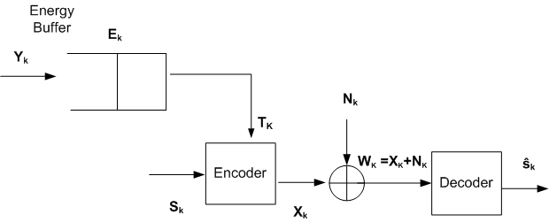
Figure 1: The model

In this section we present our model for a single energy harvesting sensor node.We consider a sensor node (Fig. 1) which is sensing and generating data to be transmitted to a central node via a discrete time AWGN channel. We assume that transmission consumes most of the energy in a sensor node and ignore other causes of energy consumption (this is true for many low quality, low rate sensor nodes ([12])). This assumption will be removed in Section IV. The sensor node is able to replenish energy by $Y_{k}$ at time $k$. The energy available in the node at time $k$ is $E_{k}$. This energy is stored in an energy buffer with an infinite capacity. In this section the fading effects are not considered; however this issue is addressed in Section VI.

The node uses energy $T_{k}$ at time $k$ which depends on $E_{k}$ and $T_{k}\leq E_{k}$ . The process $\{E_{k}\}$ satisfies

$$E_{k+1}=(E_{k}-T_{k})+Y_{k}.$$ (1)

We will assume that $\{Y_{k}\}$ is stationary ergodic. This assumption is general enough to cover most of the stochastic models developed for energy harvesting. Often the energy harvesting process will be time varying (e.g., solar cell energy harvesting will depend on the time of day). Such a process can be approximated by piecewise stationary processes. As in [18], we can indeed consider $\{Y_{k}\}$ to be periodic, stationary ergodic.

The encoder receives a message $S$ from the node and generates an $n$-length codeword to be transmitted on the AWGN channel. The channel output $W_{k}=X_{k}+N_{k}$ where $X_{k}$ is the channel input at time $k$ and $N_{k}$ is independent, identically distributed (iid) Gaussian noise with zero mean and variance $\sigma^{2}$ (we denote the corresponding Gaussian density by $\mathcal{N}(0,\sigma^{2}))$. The decoder receives $W^{n}\stackrel{{\scriptstyle\Delta}}{{=}}(W_{1},...,W_{n})$ and reconstructs $S$ such that the probability of decoding error is minimized.

We will obtain the information-theoretic capacity of this channel. This of course assumes that there is always data to be sent at the sensor node (this assumption will be removed in section VII). This channel is essentially different from the usually studied systems in the sense that the transmit power and coding scheme can depend on the energy available in the energy buffer at that time.

A possible generalization of our model is that the energy $E_{k}$ changes at a slower time scale than a channel symbol transmission time, i.e., in equation (1) $k$ represents a time slot which consists of $m$ channel uses, $m\geq 1$. We comment on this generalization in Section III (see also Section VII).

III Capacity for the Ideal System

In this section we obtain the capacity of the channel with an energy harvesting node under ideal conditions of infinite energy buffer and energy consumption in transmission only.

The system starts at time $k=0$ with an empty energy buffer and $E_{k}$ evolves with time depending on $Y_{k}$ and $T_{k}$. Thus $\{E_{k},~{}k\geq 0\}$ is not stationary and hence $\{T_{k}\}$ may also not be stationary. In this setup, a reasonable general assumption is to expect $\{T_{k}\}$ to be asymptotically stationary. Indeed we will see that it will be sufficient for our purposes. These sequences are a subset of Asymptotically Mean Stationary (AMS) sequences , i.e., sequences $\{T_{k}\}$ such that

$$\lim_{n\to\infty}\frac{1}{n}\sum_{k=1}^{n}P[T_{k}\in A]=\overline{P}(A)$$ (2)

exists for all measurable $A$. In that case $\overline{P}$ is also a probability measure and is called the stationary mean of the AMS sequence ([30]).

If the input $\{X_{k}\}$ is AMS and ergodic, then it can be easily shown that for the AWGN channel $\{(X_{k},W_{k}),~{}k\geq 0\}$ is also AMS an ergodic. In the following theorem we will show that the channel capacity of our system is ([30])

$$C=\sup_{p_{x}}\overline{I}(X;W)=\sup_{p_{x}}~{}\limsup_{n\to\infty}\frac{1}{n}I(X^{n},W^{n})$$ (3)

where $\{X_{n}\}$ is an AMS sequence, $X^{n}=(X_{1},...,X_{n})$ and the supremum is over all possible AMS sequences $\{X_{n}\}$. In other words, one can find a sequence of codeword s with code length $n$ and rate $R$ such that the average probability of error goes to zero as $n\to\infty$ if and only of $R<C$.

Theorem 1: For the energy harvesting system, the capacity $C=0.5~{}\log(1+\frac{E[Y]}{\sigma^{2}})$.

Proof: See Appendix A. This result has also appeared in [28]. The achievability proofs are somewhat different (both the scheme itself as well as the technical approach to the proof).

Thus we see that the capacity of this channel is the same as that of a node with average energy constraint $E[Y]$, i.e., the hard energy constraint of $E_{k}$ at time $k$ does not affect its capacity. The capacity achieving signaling in the above theorem is truncated $iid$ Gaussian with zero mean and variance $E[Y]$ where the truncation occurs due to the energy limitation $E_{k}$ at time $k$. The same capacity is obtained for any other initial energy $E_{0}$ (because then also our signaling scheme leads to an AMS sequence with the same stationary mean).

The scenario when there is no energy buffer to store the harvested energy (Harvest-Use) was studied extensively in [39], which calculated the capacity to be $C=\max_{p_{x}}I(X;W)\leq 0.5~{}\log(1+E[Y]/\sigma^{2})$. We mention this result in some detail (and variations) since this material will be used in developing later sections. The last inequality is strict unless $X_{k}$ is $\mathcal{N}(0,E[Y])$ and $Y_{k}$ is also known at the receiver at time $k$. Then $X^{2}=Y$ and hence $Y_{k}$ is chi-square distributed with degree 1. If $Y_{k}\equiv E[Y]$ then the capacity will be that of an AWGN channel with peak and average power constraint $=E[Y]$. This problem is addressed in [40], [41], [42] and the capacity achieving distribution is finite and discrete. Let $X(y)$ denote a random variable having distribution that achieves capacity with peak power $y$. Then, for the case when information about $Y_{k}$ is also available at the decoder at time $k$, the capacity of the channel when $\{Y_{k}\}_{k\geq 1}$ is $iid$ is

$$C=E_{Y}[I(X(Y);W)].$$ (4)

For small $y$, $X^{2}(y)=y$. This result can be extended to the case when $\{Y_{k}\}$ is stationary ergodic. Then the right side of (4) will be replaced by the information rate of $\{X_{k}(Y_{k}),W_{k}\}$. In conclusion, having some energy buffer to store the harvested energy almost always strictly increases the capacity of the system (under ideal conditions of this section).

Next we extend this result to the case when only partial information about $Y_{k}$ is available at the encoder and the decoder at time $k$ (causally). The interesting case of $Y_{k}$ information being perfectly available at the encoder and not at the decoder is a special case of this set up. The channel is given in Fig. 2 where $V^{(t)}_{k}$ and $V^{(r)}_{k}$ denote the partial information about $Y_{k}$ at the encoder and the decoder respectively. For simplicity, we will assume $\{Y_{k}\}$ to be $iid$. The capacity of this channel can be obtained from the capacity of a state dependent channel with partial state information at the encoder and the decoder ([43]):

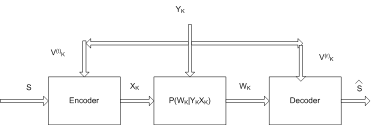
Figure 2: Capacity with no buffer and partial energy harvesting information

$$C=\sup_{P_{T}(.)}I(T;W|V^{(r)}),$$ (5)

where the supremum is over distributions $P_{T}(.)$ of continuous functions, $T\in\mathcal{T}$, $T:\mathcal{V}^{(t)}\to\mathcal{X}$ where $\mathcal{V}^{(t)}$ and $\mathcal{X}$ denote the sets in which $Y$ and $X$ take values. $\mathcal{T}$ denotes the set of all $|\mathcal{X}|^{|\mathcal{V}^{(t)}|}$ functions from $\mathcal{V}^{(t)}$ to $\mathcal{X}$. Also, $T$ is independent of $V^{(t)}$ and $V^{(r)}$. The capacity when $Y_{k}$ is not available at the decoder but perfectly known at the encoder is obtained by substituting $V^{(t)}_{k}=Y_{k}$ and $V^{(r)}_{k}=\phi$ in (5).

In [18], a system with a data buffer at the node which stores data sensed by the node before transmitting it, is considered. The stability region (for the data buffer) for the ’no-buffer’ and ’infinite-buffer’ corresponding to the harvest-use and harvest-store-use architectures are provided. The throughput optimal policies in [18] are $T_{n}=\min(E_{n};E[Y]-\epsilon)$ for the infinite energy buffer and $T_{n}=Y_{n}$ when there is no energy buffer. Hence we see that the Shannon capacity achieving energy management policies provided here are close to the throughput optimal policies in [18]. Also the capacity is the same as the maximum throughput obtained in the data-buffer case in [18] for the infinite buffer architecture. In section VII we will connect further this model with our information theoretic model studied above.

Above we considered the cases when there is infinite energy buffer or when there is no buffer at all. However, in practice often there is a finite energy buffer to store. This case is considered in Section VIII and we provide achievable rates.

Next we comment on the capacity results when (1) represents $E_{k+1}$ at the end of the $k$th slot where a slot represents $m$ channel uses. In this case energy $E_{k}$ is available not for one channel use but for $m$ channel uses. This relaxes our energy constraints. Thus if $E[Y]$ still denotes mean energy harvested per channel use, then for infinite buffer case the capacity remains same as in Theorem 1.

IV Capacity with Processor Energy (PE)

Till now we have assumed that all the energy that a node consumes is for transmission. However, sensing, processing and receiving (from other nodes) also require significant energy, especially in recent higher-end sensor nodes ([12]). We will now include the energy consumed by sensing and processing only.

We assume that energy $Z_{k}$ is consumed by the node (if $E_{k}\geq Z_{k}$) for sensing and processing at time instant $k$. Thus, for transmission at time $k$, only $E_{k}-Z_{k}$ is available. $\{Z_{k}\}$ is assumed a stationary, ergodic sequence. The rest of the system is as in Section II.

First we extend the achievable policy in Section III to incorporate this case. The signaling scheme $X_{k}=sgn(X_{k}^{\prime})\min(\sqrt{E_{k}},|X_{k}^{\prime}|)$ where $\{X_{k}^{\prime}\}$ is $iid$ Gaussian with zero mean and variance $E[Y]-E[Z]-\epsilon$ achieves the rate

$$R_{PE}=0.5~{}\log\left(1+\frac{E[Y]-E[Z]-\epsilon}{\sigma^{2}}\right).$$ (6)

If the sensor node has two modes: Sleep and Awake then the achievable rates can be improved. The sleep mode is a power saving mode in which the sensor only harvests energy and performs no other functions so that the energy consumption is minimal (which will be ignored). If $E_{k}<Z_{k}$ then we assume that the node will sleep at time $k$. But to optimize its transmission rate it can sleep at other times also. We consider a policy called randomized sleep policy in [20]. In this policy at each time instant $k$ with $E_{k}\geq Z_{k}$ the sensor chooses to sleep with probability $p$ independent of all other random variables. We will see that such a policy can be capacity achieving in the present context.

With the sleep option we will show that the capacity of this system is

$$C=\sup_{p_{x}:E[b(X)]\leq E[Y]}I(X;W),$$ (7)

where $b(x)$ is the cost of transmitting $x$ and equals

$$b(x)=\begin{cases}x^{2}+\alpha,~{}&\text{if $|x|>0$},\\ 0,~{}&\text{if $|x|=0$},\end{cases}$$

and $\alpha=E[Z]$. Observe that if we follow a policy that unless the node transmits, it sleeps, then $b$ is the cost function. An optimal policy will have this characteristic. Denoting the expression in (7) as $C(E[Y])$, we can easily check that $C(.)$ is a non-decreasing function of $E[Y]$. We also show below that $C(.)$ is concave. These facts will be used in proving that (7) is the capacity of the system.

To show concavity, for $s_{1},s_{2}>0$ and $0\leq\lambda\leq 1$ we want to show that $C(\lambda s_{1}+(1-\lambda)s_{2})\geq\lambda C(s_{1})+(1-\lambda)C(s_{2})$. For $s_{i}$, let $C_{i}$ be the capacity achieving codebook, $i=1,2$. Use $\lambda$ fraction of time $C_{1}$ and $1-\lambda$ fraction $C_{2}$. Then the rate achieved is $\lambda C(s_{1})+(1-\lambda)C(s_{2})$ while the average energy used is $\lambda s_{1}+(1-\lambda)s_{2}$. Thus, we obtain the inequality showing concavity.

Theorem 2 For the energy harvesting system with processing energy,

$$C=\sup_{p_{x}:E[b(X)]\leq E[Y]}I(X;W)$$ (8)

is the capacity for the system.

Proof: : See Appendix B.

It is interesting to compute the capacity (8) and the capacity achieving distribution. Without loss of generality, the node sleeps with probability $p,(0\leq p\leq 1)$ and with probability $(1-p)$ the node transmits with a distribution $F_{t}(.)$. We can write the overall input distribution, $F_{in}(.)$, as a mixture distribution

$$F_{in}(.)=pu(.)+(1-p)F_{t}(.),$$

where $u(.)$ denotes the unit step function. The corresponding output density function $f_{W}(.;F_{t})=pf_{N}(.)+(1-p)\int f_{N}(.-s)dF_{t}(s)$, is the convolution of $F_{in}(.)$ and $f_{N}(.)$ where $f_{N}(.)$ is $\mathcal{N}(0,\sigma^{2})$. The mutual information $I(X;W)$ in (8) can be written as

$$I(F_{t})\triangleq I(X;W)=ph(0;F_{t})+(1-p)\int h(x;F_{t})dF_{t}(x)-h(N),$$

where $h(N)$ is the differential entropy of noise $N$ and $h(x;F_{t})$ is the marginal entropy function defined as

$$h(x;F_{t})=-\int f_{N}(w-x)\log(f_{W}(w;F_{t}))dw.$$

Capacity computation can be formulated as a constrained maximization problem,

$$\sup_{F_{t}\in\Omega}I(F_{t}),$$ (9)

where $\Omega\triangleq\{F_{t}:F_{t}\text{ is a cdf and}\int s^{2}dF_{t}(s)\leq\beta_{p}\}$ and $\beta_{p}\triangleq\frac{E[Y]}{(1-p)}-\alpha$. $\Omega$ is the space of all distribution functions with finite second moments and is endowed with the topology of weak^∗ convergence. This topology is metrizable with Prohorov metric ([44]). It is easy to see that $\Omega$ is a compact, convex topological space. The compactness of $\Omega$ is a consequence of the second moment constraint of the distribution function which makes it tight and Helly’s theorem. The objective function $I(F_{t})$ is a strictly concave map from $\Omega$ to $\mathbb{R}^{+}$, the positive real line. We can show that $I(F_{t})$ is a continuous function in the weak^∗ topology and $I(F_{t})$ admits a weak derivative [40]. Then there is a unique distribution $F_{t0}$ that optimizes (9). The weak derivative of $I(F_{t})$ with respect to $F_{t}$ at the optimum distribution $F_{t0}$ is

$$I^{\prime}_{F_{t0}}(F_{t})=ph(0;F_{t0})+(1-p)\int h(x;F_{t0})dF_{t}(x)-h(N)-I(F_{to}).$$

Here, $I(F_{to})$ is the capacity of the channel. Using KKT conditions we get sufficient and necessary conditions as $I^{\prime}_{F_{t0}}(F_{t})\leq 0$ and the conditions can be simplified using the techniques in [40], [45] as

$$Q(x)\triangleq(1-p)h(x;F_{t0})+K-\lambda x^{2}\leq 0,\forall x$$ (10)

and,

$$(1-p)h(x;F_{t0})+K-\lambda x^{2}=0,\forall x\in\mathcal{S}_{0},$$ (11)

where $K=ph(0;F_{t0})-h(N)-I(F_{to})+\lambda\beta_{p}$, $\lambda\geq 0$ is the Lagrangian multiplier and $\mathcal{S}_{0}$ is the support set of the optimum distribution.

The capacity achieving distribution is discrete and can be proved using the techniques provided in [40] and is omitted for brevity. The key steps of the proof include:

• Identify the function $Q(x)$ which gives a necessary and sufficient condition for optimality.

• Show that $Q(x)$ has an analytic extension $Q(z)$ over the whole complex plane.

• Prove by contradiction that the zero set of $Q(z)$ cannot have limit points in its domain of definition and is at most countable.

Since any mass point $x$ of the optimum distribution function satisfies the condition $Q(x)=0$ the number of mass points of the optimum distribution is at most countable.

Hence we find that the optimum input distribution is not Gaussian. To get further insight, consider $\{B_{k}\}$ to be $iid$ binary random variables with $P[B_{1}=0]=p=1-P[B_{1}=1]$ and let $\{G_{k}\}$ be $iid$ random variables with distribution $F$. Then $X_{k}^{\prime}=B_{k}G_{k}$ is the capacity achieving $iid$ sequence. Also,

$$I(X_{k}^{\prime};X_{k}^{\prime}+N_{k}) = h(B_{k}G_{k}+N_{k})-h(N_{k})$$

$$= h(B_{k}G_{k}+N_{k})-h(B_{k}G_{k}+N_{k}|B_{k})+h(B_{k}G_{k}+N_{k}|B_{k})-h(N_{k})$$

$$= I(B_{k};B_{k}G_{k}+N_{k})+I(G_{k};B_{k}G_{k}+N_{k}|B_{k})$$

$$= I(B_{k};B_{k}G_{k}+N_{k})+(1-p)I(G_{k};G_{k}+N_{k}).$$ (13)

This representation suggests the following interpretation (and coding theoretic implementation) of the scheme: the overall code is a superposition of a binary ON-OFF code and an $iid$ code with distribution $F$. The position of the ON (and OFF) symbols is used to reliably encode $I(B;BG+N)$ bits of information per channel use, while the code with distribution $F$ (which is used only during the ON symbols) reliably encodes $(1-p)I(G;G+N)$ bits of information per channel use.

It is interesting to compare this result with the capacity in [31]. The capacity result in [31] is only the second term in (13) evaluated with $G_{k}$ being Gaussian.

In Fig.3 we compare the optimal sleep-wake policy, a sleep wake policy with $F$ being mean zero Gaussian with variance $E[Y]/(1-p)-\alpha$ and no-sleep policy with the result in [31]. We take $E[Z]=0.5$ and $\sigma^{2}=1$.

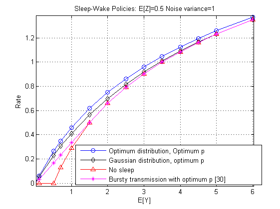
Figure 3: Comparison of Sleep Wake policies

We see that when $E[Y]$ is comparable or less than $E[Z]$ then the node chooses to sleep with a high probability. When $E[Y]>>E[Z]$ then the node will not sleep at all. Also it is found that when $E[Y]<E[Z]$, the capacity is zero when the node does not have a sleep mode. However we obtain a positive capacity if it is allowed to sleep. When $E[Y]>>E[Z]$, the optimal distribution $F$ tends to a Gaussian distribution with mean zero and variance $E[Y]-\alpha$.

From the figure we see that our scheme improves the capacity provided in [31]. This is due to the embedded binary code and the difference is significant at low values of $E[Y]$.

V Achievable Rate with Energy Inefficiencies

In this section we make our model more realistic by taking into account the inefficiency in storing energy in the energy buffer and the leakage from the energy buffer ([15]) for HSU architecture. For simplicity, we will ignore the energy $Z_{k}$ used for sensing and processing.

We assume that if energy $Y_{k}$ is harvested at time $k$, then only energy $\beta_{1}Y_{k}$ is stored in the buffer and energy $\beta_{2}$ gets leaked in each slot where $0<\beta_{1}\leq 1$ and $0<\beta_{2}<\infty$. Then (1) become

$$E_{k+1}=((E_{k}-T_{k})-\beta_{2})^{+}+\beta_{1}Y_{k}.$$ (14)

The energy can be stored in a supercapacitor and/or in a battery. For a supercapacitor, $\beta_{1}\geq 0.95$ and for the Ni-MH battery (the most commonly used battery) $\beta_{1}\sim 0.7$. The leakage $\beta_{2}$ for the battery is close to 0 but for the super capacitor it may be somewhat larger.

In this case, similar to the achievability of Theorem 1 we can show that

$$R_{HSU}=0.5~{}\log\left(1+\frac{\beta_{1}E[Y]-\beta_{2}}{\sigma^{2}}\right)$$ (15)

is achievable. This policy is neither capacity achieving nor throughput optimal [18]. An achievable rate of course is (4) (obtained via HU). Now one does not even store energy and $\beta_{1},~{}\beta_{2}$ are not effective. The upper bound $0.5~{}\log(1+{E[Y]}/{\sigma^{2}})$ is achievable if $Y$ is chi-square distributed with degree 1. Now, unlike in Section III, the rate achieved by the HU may be larger than (15) for certain range of parameter values and distributions.

Another achievable policy for the system with an energy buffer with storage inefficiencies is to use the harvested energy $Y_{k}$ immediately instead of storing in the buffer. The remaining energy after transmission is stored in the buffer. We call this Harvest-Use-Store (HUS) architecture. For this case, (14) becomes

$$E_{k+1}=((E_{k}+\beta_{1}(Y_{k}-T_{k})^{+}-(T_{k}-Y_{k})^{+})^{+}-\beta_{2})^{+}.$$ (16)

Compute the largest constant $c$ such that $\beta_{1}E[(Y_{k}-c)^{+}]>E[(c-Y_{k})^{+}]+\beta_{2}$. This is the largest $c$ such that taking $E[T_{k}]<c$ will make $E_{k}\to\infty~{}a.s.$ Thus, as in Theorem 1, we can show that rate

$$R_{HUS}=0.5~{}\log\left(1+\frac{c}{\sigma^{2}}\right)$$ (17)

is achievable for this system. This is achievable by an input with distribution $iid$ Gaussian with mean zero and variance $c$.

Equation (14) approximates the system where we have only rechargable battery while (16) approximates the system where the harvested energy is first stored in a supercapacitor and after initial use transferred to the battery.

When $\beta_{1}=1,\beta_{2}=0$ we have obtained the capacity of this system in Section III. For the general case, its capacity is an open problem.

We illustrate the achievable rates mentioned above via an example.

Example 1
Let $\{Y_{k}\}$ be $iid$ taking values in $\{0.25,0.5,0.75,1\}$ with equal probability. We take the loss due to leakage, $\beta_{2}=0$. In Figure 4 we compare the various architectures discussed in this section for varying storage efficiency $\beta_{1}$. We use the result in [42] for computing the capacity in (4).

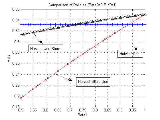
Figure 4: Rates for various architectures

From the figure it can be seen that if the storage efficiency is very poor it is better to use the $HU$ policy. This requires no storage buffer and has a simpler architecture. If the storage efficiency is good $HUS$ policy gives the best performance. For $\beta_{1}=1$, the $HUS$ policy and $HSU$ policy have the same performance. Thus if we judiciously use a combination of a supercapacitor and a battery, we may obtain a better performance.

VI Fading AWGN Channel

In this section we extend the results of Theorem 1 to include fading. Rest of the notation is same as in Section III. The model considered is given in Figure 5.

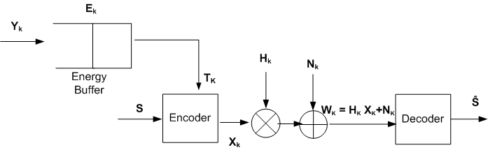
Figure 5: The model

The encoder receives a message $S$ from the node and generates an $n$-length codeword to be transmitted on the fading AWGN channel. We assume flat, fast, fading. At time $k$ the channel gain is $H_{k}$ and takes values in $\mathcal{H}$. The sequence $\{H_{k}\}$ is assumed $iid$, independent of the energy generation sequence $\{Y_{k}\}$. The channel output at time $k$ is $W_{k}=H_{k}X_{k}+N_{k}$ where $X_{k}$ is the channel input at time $k$ and $\{N_{k}\}$ is iid Gaussian noise with zero mean and variance $\sigma^{2}$. The decoder receives $Y^{n}\stackrel{{\scriptstyle\Delta}}{{=}}(Y_{1},...,Y_{n})$ and reconstructs $S$ such that the probability of decoding error is minimized. Also, the decoder has perfect knowledge of the channel state $H_{k}$ at time $k$.

If the channel input $\{X_{k}\}$ is AMS ergodic, then it can be easily shown that for the fading AWGN channel $\{(X_{k},W_{k}),~{}k\geq 0\}$ is also AMS ergodic. Thus the channel capacity of the fading system is ([30])

$$C=\sup_{p_{x}}\overline{I}(X;W)=\sup_{p_{x}}~{}\limsup_{n\to\infty}\frac{1}{n}I(X^{n},W^{n})$$ (18)

where under $p_{x}$, $\{X_{n}\}$ is an AMS sequence, $X^{n}=(X_{1},...,X_{n})$ and the supremum is over all possible AMS sequences $\{X_{n}\}$. For a fading AWGN channel, capacity achieving $X_{k}$ is zero mean Gaussian with variance $T_{k}$ where $T_{k}$ depends on the power control policy used and is assumed AMS. Then $E[T]\leq E[Y]$ where $E[T]$ is the mean of $T$ under its stationary mean. The following theorem shows that one can find a sequence of codeword s with code length $n$ and rate $R$ such that the average probability of error goes to zero as $n\to\infty$ if and only if $R<C$ where $C$ is given in (19).

Theorem 3 For the energy harvesting system with perfect CSIT,

$$C=0.5~{}E_{H}\left[\log(1+\frac{H^{2}T^{*}(H)}{\sigma^{2}})\right],$$ (19)

where

$$T^{*}(H)=\left(\frac{1}{H_{0}}-\frac{1}{H}\right)^{+},$$ (20)

and $H_{0}$ is chosen such that $E_{H}[T^{*}(H)]=E[Y]$.

Proof: See Appendix C.

Thus we see that the capacity of this fading channel is same as that of a node with average power constraint $E[Y]$ and the instantaneous power allocated is according to ‘water filling’ power allocation. The hard energy constraint of $E_{k}$ at time $k$ does not affect its capacity. The capacity achieving signaling for our system is $X_{k}=sgn(X_{k}^{\prime})\min(\sqrt{T^{*}(H_{k})}|X_{k}^{\prime}|,\sqrt{E_{k}})$, where $\{X_{k}^{\prime}\}$ is $iid$ $\mathcal{N}(0,1)$ and $T^{*}(H)$ is defined in (20).

When no CSI is available at the transmitter (but perfect CSI is available at the decoder), take $X_{k}=sgn(X_{k}^{\prime})\min(|X_{k}^{\prime}|,\sqrt{E_{k}})$ where $\{X_{k}^{\prime}\}$ is $iid$ $\mathcal{N}(0,E[Y])$ and as in Theorem 1 this approaches the capacity of $0.5~{}E_{H}[\log(1+{H^{2}E[Y]}/{\sigma^{2}})]$.

Similar to the non-fading case the throughput optimal policies in [18] are related to the Shannon capacity achieving energy management policies provided here for the infinite buffer case. Also the capacity is the same as the maximum throughput obtained in the data-buffer case in [18].

If there is no energy buffer to store the harvested energy then at time $k$ only $Y_{k}$ energy is available. Thus $X_{k}$ is peak power limited to $Y_{k}$. The capacity achieving distribution for an AWGN channel with peak power constraint $Y_{k}=y$ is not Gaussian. Let $X(y,\sigma^{2})$ be a random variable with the capacity achieving distribution for an AWGN channel with peak power constraint $y$ and noise variance $\sigma^{2}$. In general this distribution is discrete. Thus, if CSIT is exact then the transmitter will transmit $X(y,\sigma^{2}/h^{2})$ at time $k$ when $Y_{k}=y$ and $H_{k}=h$. Therefore the ergodic capacity with $Y_{k}$ information being available at the receiver is $0.5E_{YH}[I(X(Y,\sigma^{2}/H^{2});W)]$. If there is no CSIT then we can transmit $X(y,\sigma^{2})$ and the corresponding capacity is $0.5E_{YH}[I(X(Y,\sigma^{2});W)]$.

VI-A Capacity with Energy Consumption in Sensing and Processing

In this section we extend the results in Section IV to the fading case.

First we extend the achievable policies given above to incorporate the energy consumption in activities other than transmission. We assume perfect CSIR for the channel state $H_{k}$ at the time $k$. When there is perfect CSIT also, we use the signaling scheme $X_{k}=sgn(X_{k}^{\prime})\min(\sqrt{T^{*}(H_{k})}|X_{k}^{\prime}|,\sqrt{E_{k}})$, where $\{X_{k}^{\prime}\}$ is $iid$ $\mathcal{N}(0,1)$ and $T^{*}(H)$ is the optimum power allocation such that $E[T^{*}(H)]=E[Y]-E[Z]-\epsilon$. When no CSI is available at the transmitter, we use $X_{k}=sgn(X_{k}^{\prime})\min(|X_{k}^{\prime}|,\sqrt{E_{k}})$ where $\{X_{k}^{\prime}\}$ is $iid$ $\mathcal{N}(0,E[Y]-E[Z]-\epsilon)$. The achievable rates for CSIT and no CSIT respectively are,

$$R_{PE-CSIT}=0.5~{}E_{H}\left[\log\left(1+\frac{H^{2}T^{*}(H)}{\sigma^{2}}\right)\right],$$ (21)

$$R_{PE-NCSIT}=0.5~{}E_{H}\left[\log\left(1+\frac{H^{2}(E[Y]-E[Z]-\epsilon)}{\sigma^{2}}\right)\right].$$ (22)

When Sleep Wake modes are supported the achievable rates can be improved as in Section IV.

Theorem 4 Let $\mathcal{P}(H)$ be the set of all feasible power allocation policies such that for $P(H)\in\mathcal{P}(H)$, $E_{H}[P(H)]\leq E[Y]$. For the energy harvesting system with processing energy transmitting over a fading Gaussian channel,

$$C=\sup_{P(H)\in\mathcal{P}(H)}~{}\sup_{p_{x}:E[b(X)]\leq P(H)}E[I(X;W)]$$ (23)

is the capacity for the system.

Proof: : See Appendix D.

We compute the capacity (23) and the capacity achieving distribution. Let $P^{*}(h)$ be the power allocated in state $h$. Without loss of generality, under $H=h$, the node sleeps with probability $p,(0\leq p\leq 1)$ and with probability $(1-p)$ the node transmits with a distribution $F_{t}(.)$. As in Section IV, we can show using KKT conditions that the capacity achieving distribution for state $H=h$ is discrete and the number of mass points are at most countable with $E[b(X)]\leq P(h)$. As in the case without fading the distribution $F_{t}(.)$ under $H=h$ is not Gaussian.

The optimal power allocation policy $P^{*}(H)$ that maximizes (23) is not ’water filling’ but similar and uses more power when the channel is better.

Example 2

Let the fade states take values in $\{0.5,~{}1,~{}1.2\}$ with probabilities $\{0.1,~{}0.7,~{}0.1\}$. We take $\alpha=E[Z]=0.5,~{}\sigma^{2}=1$. We compare the capacity for the cases with perfect and no CSIT when there is no sleep mode supported (Equation (21), (6)) and with the optimal sleep probability in Figure 6.

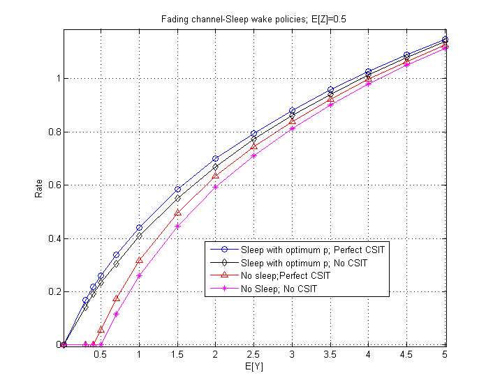
Figure 6: Comparison of sleep wake policies

From the figure we observe that

• The randomized sleep wake policy improves the rate significantly when $E[Y]\leq E[Z]$.

• The sensor node chooses not to sleep when $E[Y]>>E[Z]$.

VI-B Achievable Rate with Energy Inefficiencies

In this section we take into account the inefficiency in storing energy in the energy buffer and the leakage from the energy buffer. The notation is same as in Section V.

The energy evolves as

$$E_{k+1}=((E_{k}-T_{k})-\beta_{2})^{+}+\beta_{1}Y_{k}.$$ (24)

In this case, similar to the achievability of Theorem 3 we can show that the rates

$$R_{S-NCSIT}=0.5~{}E_{H}\left[\log\left(1+\frac{H^{2}(\beta_{1}E[Y]-\beta_{2})}{\sigma^{2}}\right)\right],$$ (25)

$$R_{S-CSIT}=0.5~{}E_{H}\left[\log\left(1+\frac{H^{2}(\beta_{1}T(H)-\beta_{2})}{\sigma^{2}}\right)\right],$$ (26)

are achievable in the no CSIT and perfect CSIT case respectively, where $T(H)$ is a power allocation policy such that (26) is maximized subject to $E_{H}[T(H)]\leq E[Y]$. This policy is neither capacity achieving nor throughput optimal [18].

An achievable rate when there is no buffer and perfect CSIT is

$$C=E_{YH}[I(X(Y,H);W)],$$ (27)

where $X(y,h)$ is the distribution that maximizes the capacity subject to peak power constraint $y$ and fade state $h$. A numerical method to evaluate the capacity with peak power constraints is provided in [40]. It is also shown in [42] that for $\sqrt{y}<1.05$, the capacity has a closed form expression

$$C(y)=y-\int_{-\infty}^{\infty}\frac{e^{-x^{2}/2}\log{cosh(y-\sqrt{y}x)}}{\sqrt{2\pi}}dx.$$ (28)

When there is no buffer and no CSIT the distribution that maximizes the capacity cannot be chosen as in (27) and the capacity is less than the capacity given in (27). The capacity in (27) is without using buffer and hence $\beta_{1}$ and $\beta_{2}$ do not affect the capacity. Hence unlike in Section III, (27) may be larger than (25) and (26) for certain range of parameter values. We will illustrate this by an example.

For the Harvest-Use-Store (HUS) architecture, (24) becomes

$$E_{k+1}=((E_{k}+\beta_{1}(Y_{k}-T_{k})^{+}-(T_{k}-Y_{k})^{+})^{+}-\beta_{2})^{+}.$$ (29)

Find the largest constant $c$ such that $\beta_{1}E[(Y_{k}-c)^{+}]\geq E[(c-Y_{k})^{+}]+\beta_{2}$. Of course $c<E[Y]$. When there is no CSIT, this is the largest $c$ such that taking $T_{k}=\min(c-\delta,E_{k})$, where $\delta>0$ is any small constant, will make $E_{k}\to\infty~{}a.s.$ and hence $T_{k}\to c~{}a.s.$ Then, as in Theorem 3, we can show that

$$R_{US-NCSIT}=0.5~{}E_{H}\left[\log\left(1+\frac{H^{2}c}{\sigma^{2}}\right)\right]$$ (30)

is an achievable rate.

When there is perfect CSIT, ’water filling’ power allocation can be done subject to average power constraint of $c$ and the achievable rate is

$$R_{US-CSIT}=0.5~{}E_{H}\left[\log\left(1+\frac{H^{2}T^{*}(H)}{\sigma^{2}}\right)\right]$$ (31)

where $T^{*}(H)$ is the ’water filling’ power allocation with $E[T^{*}(H)]=c$.

We illustrate the achievable rates mentioned above via an example.

Example 3

Let the process $\{Y_{k}\}$ be $iid$ taking values in $\{0.5,~{}1\}$ with probability $\{0.6,~{}0.4\}$ . We take the loss due to leakage $\beta_{2}=0$. The fade states are $iid$ taking values in $\{0.4,~{}0.8,~{}1\}$ with probability $\{0.4,~{}0.5,~{}0.1\}$. In Figure 7 we compare the various architectures discussed in this section for varying storage efficiency $\beta_{1}$. The capacity for the no buffer case with perfect CSIT is computed using equations (28) and (27).

Figure 7: Rates for various architectures

From the figure we observe

• Unlike the ideal system, the $HSU$ (which uses infinite energy buffer) performs worse than the $HU$ (which uses no energy buffer) when storage efficiency is poor for the perfect CSIT case.

• When storage efficiency is high, $HU$ policy performs worse compared to $HSU$ and $HUS$ for perfect CSIT case.

• $HUS$ performs better than $HSU$ for No/Perfect CSIT.

• For $\beta=1$, the $HUS$ policy and $HSU$ policy are the same for both perfect CSIT and no CSIT.

• The availability of CSIT and storage architecture plays an important role in determining the achievable rates.

VII Combining Information and Queuing Theory

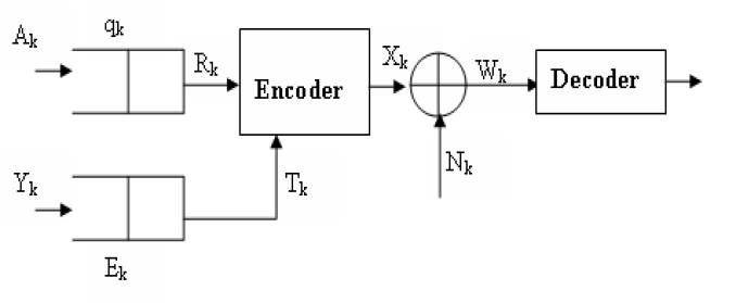
Figure 8: Model of an energy harvesting point to point channel.

In this section we consider a system with both energy and data buffer, each with infinite capacity (see Fig. 8). We consider the simplest case: no fading, no battery leakage and storage inefficiencies. The system is slotted. During slot $k$ (defined as time interval $[k,k+1]$, i.e., a slot is a unit of time), $A_{k}$ bits are generated. Although the transmitter may generate data as packets, we allow arbitrary fragmentation of packets during transmission. Thus, packet boundaries are not important and we consider bit strings (or just fluid). The bits $A_{k}$ are eligible for transmission in $(k+1)$st slot. The queue length (in bits) at time $k$ is $q_{k}$. We assume that transmission consumes most of the energy at the transmitter and ignore other causes of energy consumption. We denote by $E_{k}$ the energy available at the node at time $k$. The energy harvesting source is able to replenish energy by $Y_{k}$ in slot $k$.

In slot $k$ we will use energy

$$T_{k}=\min(E_{k},E[Y]-\epsilon),$$ (32)

where $\epsilon$ is a small positive constant. It was shown in [18] that such a policy is throughput optimal (and it is capacity achieving in Theorem 1).

There are $n$ channel uses (mini slots) in a slot, i.e., the system uses an $n$ length code to transmit the data in a slot. The length $n$ of the code word can be chosen to satisfy certain code error rate. The slot length $n$ and $R_{k}$ are to be appropriately chosen. We use codewords of length $n$ and rate $R_{k}=0.5\log(1+T_{k}/{n\sigma^{2}})$ in slot $k$ with the following coding and decoding scheme:

1) An augmented message set $\{1,...,2^{nR_{k}}\}\cup\{0\}$.

2) An encoder that assigns a codeword $x^{n}(m)$ to each $m\in\{1,...,2^{nR_{k}}\}\cup\{0\}$ where $x^{n}(m)$ is generated as an $iid$ sequence with distribution $\mathcal{N}(0,T_{k}/n-\delta_{1})$ and $\delta_{1}>0$ is a small constant. The codeword $x^{n}(m)$ is retained if it satisfies the power constraint $\sum_{i}^{n}x_{i}^{2}\leq T_{k}$. Otherwise error message 0 is sent.

3) A decoder that assigns a message $\hat{m}\in\{1,...,2^{nR_{k}}\}\cup\{0\}$ to each received sequence $w^{n}$ in a slot such that $(x^{n}(\hat{m}),w^{n})$ is jointly typical and there is no other $x^{n}(m^{\prime})$ jointly typical with $w^{n}$. Otherwise it declares an error.

In slot $k$, $nR_{k}$ bits are taken out of the queue if $q_{k}\geq nR_{k}$. The bits are represented by a message $m_{k}\in\{1,...,2^{nR_{k}}\}$ and $x^{n}(m_{k})$ is sent. If $q_{k}<nR_{k}$ no bits are taken out of the queue and “0 message” $x^{n}(0)$ is sent.

Hence the processes $\{E_{k}\}$ and $\{q_{k}\}$ satisfy

$$q_{k+1} = q_{k}-nR_{k}I_{\{q_{k}\geq nR_{k}\}}+A_{k},$$ (33)

$$E_{k+1} = (E_{k}-T_{k})+Y_{k}.$$ (34)

With $T_{k}$ in (32), $E_{k}\to\infty~{}a.s.$ and $T_{k}\to E[Y]-\epsilon~{}a.s.$ Also, $R_{k}=0.5~{}\log(1+\frac{T_{k}}{n\sigma^{2}})\to 0.5~{}\log(1+\frac{E[Y]-\epsilon}{n\sigma^{2}})$. Thus we obtain

Theorem 5. The random data arrival process $\{A_{k}\}$ can be communicated with arbitrarily low average probability of block error, by an energy harvesting sensor node over a Gaussian channel with a stable queue if and only if $E[A]<0.5n~{}\log(1+\frac{E[Y]}{n\sigma^{2}})$.                                                                          $\blacksquare$

In Theorem 5 ’stability’ of the queue has the following interpretation. If $\{A_{k}\}$ is stationary, ergodic then $P[q_{k}\to\infty]=0$ and with probability 1, $\{q_{k}\}$ visits the set $\{q:q<nR\}$ infinitely often. Also the sequence $\{q_{k}\}$ is tight ([46]). If $\{A_{k}\}$ is iid then $\{q_{k},E_{k}\}$ is a Markov chain. With $T_{k}$ in (32), asymptotically, $T_{k}\to E[Y]-\epsilon~{}a.s.$ and we can ignore the $E_{k}$ component of the process and think of $\{q_{k}\}$ as a Markov chain with $T_{k}=E[Y]-\epsilon$. It has a finite number of ergodic sets. The process $\{q_{k}\}$ eventually enters one ergodic set with probability 1 and then approaches a stationary distribution. If $\{q_{k}\}$ is irreducible and aperiodic then $\{q_{k}\}$ has a unique stationary distribution and $\{q_{k}\}$ converges in distribution to it irrespective of initial conditions.

Although the capacity achieved in each slot is as per Theorem 1, the set-up used here is somewhat different. In Theorem 1, the time scale of the dynamics of the energy process $\{E_{k}\}$ is mini slots, but in this section we have taken it at the time scale of slots (which one is the right model depends on the system under consideration). Thus, in Theorem 1 we used the theoretical tool of AMS sequences. But in our present setup, in a slot we can use $X_{1},X_{2},....,X_{n}$ $iid$ Gaussian $\mathcal{N}(0,T_{k}/n-\delta)$ and use a codeword only if it satisfies $X_{1}^{2}+....+X_{n}^{2}\leq T_{k}$ and $q_{k}\geq nR_{k}$; otherwise an error message is sent. Of course, if the physical system demands that we should use for the energy dynamics the time scale of a channel use then we can use the framework of Theorem 1.

VIII Finite Buffer

In this section we find achievable rates when the sensor node has a finite buffer to store the harvested energy. This case is of more practical interest. We consider the simplest case: no fading, no battery leakage and storage inefficiencies and no data queue. The node has an energy buffer of size $\Gamma<\infty$. By this we mean that the energy buffer can store a finite number of energy units of interest.

We use the HUS architecture where the energy harvested is used and only the left over energy is stored. The energy available at the buffer at time $k$ is denoted by $\hat{E}_{k}$. At time $k$, the node uses energy $T_{k}$ with $T_{k}\leq\hat{E}_{k}+Y_{k}\stackrel{{\scriptstyle\Delta}}{{=}}E_{k}$. We assume that $\hat{E}_{k}$ and $Y_{k}$ take values in finite alphabets. Also, $\{Y_{k}\}_{k\geq 1}$ is assumed $iid$.

We assume that the buffer state information (BSI), ${E_{k}}$, is perfectly available at the encoder and the decoder at time $k$. $X_{k}$ denotes the codeword symbol used at time $k$ and $X_{k}^{2}\leq T_{k}$. Of course $T_{k}\leq E_{k}$ and $\hat{E}_{k}\leq\Gamma$. In general $T_{k}$ is a function of $E_{0},...,E_{k}$. . An easily tractable class of energy management policies is

$$T_{k}=h(E_{k}),$$ (35)

where $h$ defines the energy management policy. The codeword symbol $X_{k}$ is picked with a distribution that maximizes the capacity of a Gaussian channel with peak power constraint $T_{k}$ (we quantize this such that $\{E_{k}\}$ takes values in a finite alphabet). Hence the process $\{E_{k}\}_{k\geq 1}$ satisfies,

$$E_{k+1}=(E_{k}-X_{k}^{2})+Y_{k+1}$$ (36)

and is a finite state Markov chain with the transition matrix decided by $h$. If $\hat{E}_{0}=0$ then the Markov chain will either enter only one ergodic set or possibly in a finite number of disjoint components which depend on $h$. If $I^{*}$ and $\overline{I}$ denote the Pinsker and Dobrushin information rates ([30]), since we have finite alphabets, $I^{*}=\overline{I}$. In particular,

$$I^{*}\big{(}X;W\big{)}{=\overline{I}\big{(}X;W\big{)}}{=\lim_{n\rightarrow\infty}~{}\frac{1}{n}I(X^{(n)};W^{(n)}).}$$ (37)

Also, Asymptotic Equi-partition Property holds for $\{X_{k},W_{k}\}$.

The following theorem provides achievable rates.

Theorem 6: A rate $R$ is achievable if an energy management policy $h$ exists, such that $R<\overline{I}\big{(}X;W)$.$\blacksquare$

The proof is similar to the achievability proof given in Theorem 1. The rates (37) can be computed via algorithms available in [47] and [48]. Using stochastic approximation ([49]) we can obtain the Markov chains that optimize (37). If initial energy $\hat{E}_{0}$ is not zero, then the Markov chain can enter some other ergodic sets and the achievable rates can be different. If $h$ is such that $\{E_{k}\}$ is an irreducible Markov chain then the achievable rates will be independent of the initial state $\hat{E}_{0}$.

Theorem 6 can be generalized to include the case where $\{(E_{k},X_{k})\}$ is a $k-$step finite state Markov chain. In fact if $\{(E_{k},X_{k})\}$ is a general AMS ergodic finite alphabet sequence then AEP holds and $I^{*}=\overline{I}$. Thus, $R<\lim_{n\to\infty}n^{-1}I(X^{n};W^{n})$ is achievable.

The capacity of our system can be written as ([50])

$$C=\sup~{}p-\liminf\frac{1}{n}log\frac{p(x^{n},w^{n})}{p(x^{n})p(w^{n})},$$ (38)

where $p-\liminf$ is defined in [50] and $\sup$ is over all input distributions $X^{n}$ which satisfy the energy constraints $X_{k}^{2}\leq E_{k}$ for all $k\geq 0$. An interesting open problem is: can (38) be obtained by limiting $\{X_{n}\}$ to AMS ergodic sequences mentioned above?

The achievable rates when the decoder has only partial information about $E_{k}$ can be handled as for the system with no buffer and partial BSI, studied in Section III.

Example 4

We consider a system with a finite buffer with $\Gamma=15$ units in steps of size 1. The $Y_{k}$ process has three mass points and provided in Table 1. We compute the optimal achievable rate using simultaneous perturbation stochastic approximation algorithm [49]. The achievable rate is also compared with a greedy policy, where the rate is evaluated using algorithms provided in [47] and [48]. In the greedy policy, at any instant $k$, an optimum distribution for an AWGN channel peak amplitude constrained to $\sqrt{E_{k}}=\sqrt{\hat{E}_{k}+Y_{k}}$ is used. We have also obtained the optimal rates using a 1-step Markov policy (35) where the optimal Markov chain is obtained via stochastic approximation. Then achievable rates are compared with the capacity with infinite buffer and no-buffer in Figure 9.

TABLE I: $Y_{k}$ Process

E(Y)	Mass points	Probabilities
0	0  0  0	1        0         0
1.0141	0   1  2	0.3192   0.3474  0.3333
2.1031	1  2  3	0.2303  0.4364  0.3333
3.3078	2  3  4	0.1794  0.3333  0.4872
4.1990	3  4  5	0.2338  0.3333  0.4329
5.0854	4  5  6	0.3333  0.2479  0.4188
5.8738	5  6  7	0.3964  0.3333  0.2703
6.7168	6  7  8	0.4749  0.3333  0.1917
8.2533	7  8  9	0.2067  0.3333  0.4600
9.0332	8  9  10	0.3167  0.3333  0.3499
9.9136	9  10  11	0.3333  0.4198  0.2469

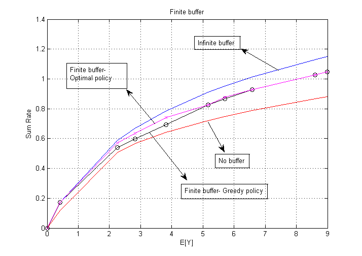
Figure 9: Acheivable rate for finite buffer

From the figure we observe that, for a given buffer size, the greedy policy is close to optimal at higher $E[Y]$. Also, the optimal achievable rates for finite buffer case are close to the capacity for infinite buffer for small $E[Y]$ but becomes close to the greedy at high $E[Y]$.

IX Conclusions

In this paper the Shannon capacity of an energy harvesting sensor node transmitting over an AWGN Channel is provided. It is shown that the capacity achieving policies are related to the throughput optimal policies. Also, the capacity is provided when energy is consumed in activities other than transmission. Achievable rates are provided when there are inefficiencies in energy storage. We extend the results to the fast fading case. We also combine the information theoretic and queuing theoretic formulations. Finally we also consider the case when the energy buffer is finite.

X Acknowledgement

The authors would like to thank Deekshith P K, PhD student, ECE, IISc for helpful inputs provided in Section IV.

Appendix A Proof of Theorem 1

Codebook Generation : Let $\{X_{k}^{\prime}\}$ be an $iid$ Gaussian sequence with mean zero and variance $E[Y]-\epsilon$ where $\epsilon>0$ is an arbitrarily small constant. For each message $s\in\{1,2,...,2^{nR}\}$, generate $n$ length codewords according to the iid distribution $\mathcal{N}(0,E[Y]-\epsilon)$. Denote the codeword by $X^{\prime n}(s)$. Disclose this codebook to the receiver.

Encoding: When $S=s$, choose the channel codeword to be $X_{k}=sgn(X_{k}^{\prime}(s))\min(\sqrt{E_{k}},|X_{k}^{\prime}(s)|)$ where $sgn(x)=1$ if $x\geq 0$ and $=-1$ if $x<0$. Then $T_{k}=X_{k}^{2}\leq E_{k}$ and $E[T_{k}]=E[X_{k}^{2}]\leq E[Y]-\epsilon$. Thus, from standard results on G/G/1 queues ([51], chapter 7) $E_{k}\to\infty~{}a.s.$ and hence $|X_{k}-X_{k}^{\prime}|\to 0~{}a.s$. Also $(X_{k},W_{k})$ converges almost surely(a.s.) to a random variable with the distribution of $(X_{k}^{\prime},W_{k}^{\prime})$ and $\{(X_{k},W_{k},X_{k}^{\prime})\}$ is AMS ergodic where $W_{k}^{\prime}=X_{k}^{\prime}+N_{k}$.

Decoding: The decoder obtains $W^{n}$ and finds the codeword $X^{\prime n}(\hat{s})$ such that $(X^{\prime n}(\hat{s}),W^{n})\in T_{\epsilon}^{n}$ where $T_{\epsilon}^{n}$ is the set of weakly $\epsilon$-typical sequences of the joint AMS ergodic distribution $P_{X^{\prime}W^{\prime}}$. If it is a unique $\hat{s}$ then it declares $\hat{s}$ as the message transmitted; otherwise declares an error.

Analysis of error events

Let $s$ has been transmitted. The following error events can happen

E1: $\{(X^{\prime n}({s}),W^{n})\notin T_{\epsilon}^{n}\}$. The probability of event E1 goes to zero as, $\{X^{\prime}_{k},W_{k}\}$ is AMS ergodic and AEP holds for AMS ergodic sequences ([52]), as $\{X^{\prime}_{k},W_{k}\}$ has a density with respect to $iid$ Gaussian measure on an appropriate Euclidean space.

E2: There exist $\hat{s}\neq s$ such that $\{(X^{\prime n}(\hat{s}),W^{n})\in T_{\epsilon}^{n}\}$. Let $\overline{H}(X^{\prime}),\overline{H}(W^{\prime})$ be the entropy rates of $\{X^{\prime}_{k}\}$ and $\{W^{\prime}_{k}\}$. Next we show that $P(E_{2})\to 0$ as $n\to\infty$. We have

$$P(E2) = \sum_{\hat{s}\neq s}P((X^{\prime n}(\hat{s}),W^{n})\in T_{\epsilon}^{n})$$

$$\leq 2^{-nR}\sum_{(x^{n},w^{n})\in T_{\epsilon}^{n}}P(x^{n},w^{n})$$

$$\leq 2^{-nR}\sum_{(x^{{}^{\prime}n},w^{\prime n})\in T_{\epsilon}^{n}}P(x^{\prime n})P(w^{\prime n})$$

$$\leq |T_{\epsilon}^{n}|2^{-nR}2^{-(n\overline{H}(X^{\prime})-\epsilon)}2^{-(n\overline{H}(W^{\prime})-\epsilon)}$$

$$\leq 2^{(n\overline{H}(X^{\prime},W^{\prime})+\epsilon)}2^{-nR}2^{-(n\overline{H}(X^{\prime})-\epsilon)}2^{-(n\overline{H}(W^{\prime})-\epsilon)}.$$

Therefore, $P(E2)\to 0$ and $n\to\infty$ if $R<\overline{I}({X^{\prime}};{W^{\prime}})=0.5\log(1+P/\sigma^{2})$.

Converse Part: For the system under consideration $\frac{1}{n}\sum_{k=1}^{n}T_{k}\leq\frac{1}{n}\sum_{k=1}^{n}Y_{k}\to E[Y]~{}a.s.$ Hence, if $\{X_{k}(s),~{}k=1,...,n\}$ is a codeword for message $s\in\{1,...,2^{nR}\}$ then for all large $n$ we must have $\frac{1}{n}\sum_{k=1}^{n}X_{k}(s)^{2}\leq E[Y]+\delta$ with a large probability for any $\delta>0$. Hence by the converse in the AWGN channel case, $\limsup_{n\to\infty}\frac{1}{n}I(X^{n};W^{n})\leq 0.5~{}\log(1+{(E[Y]+\delta)}/{\sigma^{2}})$. Now take $\delta\to 0$.

Combining the direct part and converse part completes the proof.                                                                  $\blacksquare$

Appendix B Proof of Theorem 2

Codebook Generation : For each message $s\in\{1,2,...,2^{nR}\}$, generate $n$ length codewords according to an $iid$ distribution $p_{X}^{\prime}$ with constraint $E[b(X^{\prime})]=E[Y]-\epsilon$, where $\epsilon>0$ is a small constant. Denote the codeword by $X^{\prime n}(s)$. Disclose this codebook to the receiver.

Encoding : When $S=s$, choose the channel codeword as

$$X_{k}(s)=\begin{cases}\min\{X_{k}^{\prime}(s),\sqrt{(E_{k}-Z_{k})^{+}}\},~{}&\text{if $X_{k}^{\prime}\geq 0$},\\ \max\{X_{k}^{\prime}(s),-\sqrt{(E_{k}-Z_{k})^{+}}\},~{}&\text{if $X_{k}^{\prime}<0$}.\end{cases}$$

Then to transmit $X_{k}(s)$ we need energy $T_{k}=(X_{k}^{2}+Z_{k})1_{\{X_{k}\neq 0\}}$ and $E_{k+1}=(E_{k}-T_{k})+Y_{k}$. Also,

$$E[T_{k}] = E[X_{k}^{2}]+E[Z_{k}]P\{X_{k}\neq 0\}$$

$$\leq E[X_{k}^{\prime 2}]+\alpha P\{X_{k}^{\prime}\neq 0\}={E[Y]}-\epsilon.$$

Thus, from standard results on G/G/1 queues ([51], chapter 7) $E_{k}\to\infty~{}a.s.$ and hence $|X_{k}-X_{k}^{\prime}|\to 0~{}a.s$. Also finite dimensional distributions of $\{(X_{m+k},W_{m+k},X_{m+k}^{\prime}),~{}k\geq 0\}$ converge $a.s.$ to that of $\{(X_{k}^{\prime},W_{k}^{\prime},X_{k}^{\prime})\}$. Thus $\{(X_{k},W_{k},X_{k}^{\prime})\}$ is AMS ergodic with limiting distribution $(X_{k}^{\prime},W_{k}^{\prime},X_{k}^{\prime})$ where $W_{k}^{\prime}=X_{k}^{\prime}+N_{k}$. Furthermore the energy constraints are also met.

If the chosen codeword is $\epsilon-$weakly typical and $\sum_{i=1}^{n}b(x_{i})/n\leq E[Y]-\epsilon$, then transmit it; otherwise send an error message. The probability that an error message is sent goes to zero as $n\to\infty$.

Decoding: The decoder obtains $W^{n}$. If it finds a unique codeword $X^{\prime n}(\hat{s})$ such that $\{(X^{\prime n}(\hat{s}),W^{n})\in T_{\epsilon}^{n}\}$ where, $T_{\epsilon}^{n}$ is the set of $\epsilon$-typical sequence for the distribution $P_{X^{\prime}W^{\prime}}$, it declares $\hat{s}$ as the transmitted message. Otherwise it declares an error.

By the usual methods as in Theorem 1 with the above coding-decoding scheme and also the fact that $C(.)$ is non-decreasing, we can show that the probability of error for this scheme goes to zero as $n\to\infty$. Thus we can achieve the capacity (8).

Converse: The converse follows via Fano’s inequality as in Theorem 1. For that proof to hold here, we need that $C(.)$ is concave                                                                                        $\blacksquare$

Appendix C Proof of Theorem 3

Achievability: Let $T_{k}^{\prime}=T^{*}(H_{k})$ with $T^{*}$ defined in (20) with $E[T^{*}(H)]=E[Y]-\epsilon$ where $\epsilon>0$ is a small constant. Since $\{H_{k}\}$ is $iid$, $\{T_{k}^{\prime}\}$ is also $iid$. We take $T_{k}=min(E_{k},T_{k}^{\prime})$. Thus, as in the proof of Theorem 1, from standard results on G/G/1 queues ([51], chapter 7) $E_{k}\to\infty~{}a.s.$ Therefore, as $T^{*}(H)$ is upper bounded, $\lim_{n\to\infty}\sup_{k\geq n}|T_{k}-T^{*}(H_{k})|\to 0~{}a.s.$

Let $\{X_{k}^{{}^{\prime}}\}$ be $iid$ Gaussian with mean zero and variance one. The channel codeword $X_{k}=sgn(X_{k}^{\prime})\min(\sqrt{T_{k}}|X_{k}^{\prime}|,\sqrt{E_{k}})$ where $sgn(x)=1$, if $x\geq 0$ and $-1$ otherwise. This is an AMS ergodic sequence with the stationary mean being the distribution of $\sqrt{T^{*}(H_{k})}X_{k}^{\prime}$. Then since AWGN channel under consideration is AMS ergodic ([30]), $(X,W)\stackrel{{\scriptstyle\Delta}}{{=}}\{(X_{k},W_{k}),~{}k\geq 1\}$ is AMS ergodic.

By using the techniques in Theorem 1, $R\leq\overline{I}(X,W)=0.5~{}E_{H}[\log(1+{H^{2}T^{*}(H))}/\sigma^{2})]$.

Converse Part: Let there be a sequence of codebooks for our system with rate $R$ and average probability of error going to 0 as $n\to\infty$. If $\{X_{k}(s),~{}k=1,...,n\}$ is a codeword for message $s\in\{1,...,2^{nR}\}$ then ${1}/{n}\sum_{k=1}^{n}X_{k}(s)^{2}\leq 1/n\sum_{k=1}^{n}Y_{k}\leq E[Y]+\delta$ for any $\delta>0$ with a large probability for all $n$ large enough. Hence by the converse in the fading AWGN channel case ([27]), $R<\limsup_{k\to\infty}I(X^{k};W^{k})/k\leq 0.5~{}E_{H}[\log(1+{H^{2}T^{*}(H)}/\sigma^{2})]$ for $T^{*}(H)$ given in (20).

Combining the direct and the converse part completes the proof.                                                            $\blacksquare$

Appendix D Proof of Theorem 4

Fix the power allocation policy $P^{*}$. Under $P^{*}(h)$, the achievability of $\sup_{p_{x}:E[b(X)]\leq P^{*}(h)}I(X;W)$, whenever $H_{k}=h$, is proved using the techniques provided in Theorem 2 for the non-fading case. Using this along with finding the expectation w.r.t. the optimum power allocation scheme completes the achievability proof.

The converse follows via Fano’s inequality.                                                                                $\blacksquare$

References

- [1] M. Bhardwaj and A. P. Chandrakasan, “Bounding the life time of sensor networks via optimal role assignments,” Proc. of IEEE INFOCOM 2002, pp. 1587–1598, June 2002.
- [2] S. S. Pradhan, J. Kusuma, and K. Ramachandran, “Distributed compression in a large microsensor network,” IEEE Signal Proc. Magazine, pp. 51–60, March 2002.
- [3] S. J. Baek, G. Veciana, and X. Su, “Minimizing energy consumption in large-scale sensor networks through distributed data compression and hierarchical aggregation,” IEEE JSAC, vol. 22, no. 6, pp. 1130–1140, Aug 2004.
- [4] A. Sinha and A. Chandrakasan, “Dynamic power management in wireless networks,” IEEE Design Test. Comp, April 2001.
- [5] M. Woo, S. Singh, and C. S. Raghavendra, “Power aware routing in mobile adhoc networks,” Proc. ACM Mobicom, 1998.
- [6] S. Ratnaraj, S. Jagannathan, and V. Rao, “Optimal energy-delay subnetwork routing protocol for wireless sensor networks,” IEEE Conf. on Networking, Sensing and Control, no. 787-792, April 2006.
- [7] W. Ye, J. Heidemann, and D. Estrin, “An energy efficient mac protocol for wireless sensor networks,” Proc. INFOCOM 2002.
- [8] O. Gnawal, B. Greenstein, K. Y. Jang, A. Joki, and J. Paek, “The Tenet architecture for tired sensor networks,” Proc. of the 4th International Conference on Embedded Networked Sensor Ststems, ACM, pp. 153–166, 2006.
- [9] S. Kumar, T. H. Lai, and J. Balogh, “On k-coverage of mostly sleeping sensor network,” Wireless Networks, vol. 14, no. 3, pp. 277–294, 2008.
- [10] A. Kansal, J. Hsu, S. Zahedi, and M. B. Srivastava, “Power management in energy harvesting sensor networks,” ACM. Trans. Embedded Computing Systems, 2006.
- [11] D. Niyato, E. Hossain, M. M. Rashid, and V. K. Bhargava, “Wireless sensor networks with energy harvesting technologies: A game-theoretic approach to optimal energy management,” IEEE Wireless Communications, pp. 90–96, Aug 2007.
- [12] V. Raghunathan, S. Ganeriwal, and M. Srivastava, “Emerging techniques for long lived wireless sensor networks,” IEEE Communication Magazine, pp. 108–114, April 2006.
- [13] A. Kansal and M. B. Srivastava, “An environmental energy harvesting framework for sensor networks,” International Symposium on Low Power Electronics and Design, ACM Press, pp. 481–486, 2003.
- [14] M. Rahimi, H. Shah, G. S. Sukhatme, J. Heidemann, and D. Estrin, “Studying the feasibility of energy harvesting in a mobile sensor network,” Proc. IEEE Int. Conf. on Robotics and Automation, 2003.
- [15] X. Jiang, J. Polastre, and D. Culler, “Perpetual environmentally powered sensor networks,” Proc. IEEE Conf on Information Processing in Sensor Networks, pp. 463–468, 2005.
- [16] N. Jaggi, K. Kar, and N. Krishnamurthy, “Rechargeable sensor activation under temporally correlated events,” Wireless Networks, December 2007.
- [17] H. Erkal, F. M. Ozcelik, M. A. Antepli, B. T. Bacinoglu, and E. Uysal-Biyikoglu, “A survey of recent work on energy harvesting networks,” Computer and Information sciences, Springer-Verlag, London, 2012.
- [18] V. Sharma, U. Mukherji, V. Joseph, and S. Gupta, “Optimal energy management policies for energy harvesing sensor networks,” IEEE Trans. on Wireless Communciations, vol. 9, pp. 1326–1336, 2010.
- [19] V. Joseph, V. Sharma, and U. Mukherji, “Efficient energy management policies for networks with energy harvesting sensor nodes,” Proc. 46th Annual Allerton Conference on Communication, Control and Computing, USA, 2008.
- [20] ——, “Optimal sleep-wake policies for an energy harvesting sensor node,” Proc. IEEE International Conference on Communications (ICC09), Germany, 2009.
- [21] V. Joseph, V. Sharma, U. Mukherji, and M. Kashyap, “Joint power control, scheduling and routing for multicast in multi-hop energy harvesting sensor networks,” 12th ACM International conference on Modelling, Analysis and simulation of wireless and mobile systems, Oct 2009.
- [22] R. Srivastava and C. E. Koksal, “Basic tradeoff for energy management for rechargeable sensor networks,” Submitted. Available: arxiv.org/pdf/1009.0569v2.pdf.
- [23] P. Castiglione, O. Simeone, E. Erkip, and T. Zemen, “Energy management policies for energy neutral source channel coding,” Submitted. Available: arxiv.org/pdf/1103.4787.pdf, 2011.
- [24] C. K. Ho and R. Zhang, “Optimal energy allocation for wireless communication powered by energy harvesters,” IEEE ISIT, 2010.
- [25] A. PrandehGheibi, M. Medard, A. Ozdaglar, and A. Eryilmaz, “Information theory vs queuing theory for resource allocation in multiple access channels,” IEEE PIMRC, 2008.
- [26] I. E. Teletar and R. G. Gallager, “Combining queueing theory with information theory for multiaccess,” IEEE Journal on Selected Areas in Communications, vol. 13, no. 6, pp. 963 – 969, 1995.
- [27] A. J. Goldsmith and P. P. Varaiya, “Capacity of fading channels with channel side information,” IEEE Trans. Inform. Theory, vol. 43, no. 6, pp. 1986–1992, Nov 1997.
- [28] O. Ozel and S. Ulukus, “Information-theoretic analysis of an energy harvesting communication system,” IEEE PIMRC, Sept. 2010.
- [29] R. Rajesh, V. Sharma, and P. Viswanath, “Information capacity of energy harvesting sensor nodes,” Available at Arxiv, http://arxiv.org/abs/1009.5158.
- [30] R. M. Gray, “Entropy and information theory,” Springer Verlag, 1990.
- [31] P. Y. Massaad, M. Medard, and L. Zheng, “Impact of processing energy on the capacity of wireless channels,” Proc. ISITA, Italy, 2004.
- [32] R. Rost and G. Fettweis, “Green communication in cellular network with fixed relay nodes,” to be published by Cambridge university press, Sept. 2010.
- [33] E. Altman, K. Avrachenkov, and A. Garnaev, “Taxation for green communication,” WiOpt, 2010.
- [34] C. Park and P. H. Chou, “Ambimax: Autonomous energy harvesting platform for multi supply wireless sensor nodes,” 3rd annual IEEE communication society conference on sensor and ad-hoc communication and networks, pp. 168–177, Sept. 2006.
- [35] P. Gover, K. A. Woyach, and A. Sahai, “Towards a communication theoretic understanding of system level power consumption,” IEEE JSAC, Special issue on energy efficient wireless communication, 2011.
- [36] A. Sahai and P. Grover, “The price of certainty: ”waterslide curves” and the gap to capacity,” Submitted to IEEE Trans. Information theory, Available:http://arxiv.org/abs/0801.0352.
- [37] H. Asnani, H. Permuter, and T. Weissman, “Probing capacity,” Submitted, Available: http://arxiv.org/abs/1010.1309.
- [38] S. Cui, A. Goldsmith, and A. Bahai, “Energy constrained modulation optimization,” IEEE Trans. Wireless Communication, vol. 4, no. 5, pp. 1–11, 2005.
- [39] O. Ozel and S. Ulukus, “AWGN channel under time-varying amplitude constraints with causal information at the transmitter,” 45th Asilomar Conference on Signals, Systems and Computers, Pacific Grove, CA, Nov. 2011.
- [40] J. G. Smith, “The information capacity of amplitude and variance-constrained scalar Gaussian channels,” Inform. Control, vol. 18, pp. 203–219, 1971.
- [41] S. Shamai and I. Bar-David, “The capacity of average and peak-power-limited quadrature Gaussian channel,” IEEE Trans. Inform. Theory, vol. 41, pp. 1060–1071, 1995.
- [42] M. Raginsky, “On the information capacity of Gaussian channels under small peak power constraints,” Proc. 46th Annual Allerton Conference on Communication, Control and Computing, USA, 2008.
- [43] G. Keshet, Y. Steinberg, and N. Merhav, “Channel coding in the presence of side information: Subject review,” NOW, June 2008.
- [44] R. F. Bass, “Stochastic processes,” Cambridge University Press, 2011.
- [45] I. C. Abou-Faycal, M. D. Trott, and S. Shamai, “The capacity of discrete-time memoryless rayleigh-fading channels,” IEEE Trans. Inform. Theory, vol. 47, no. 4, 2001.
- [46] P. Billingsley, “Probability and measure,” John Wiley and Sons, 3rd Ed., 1995.
- [47] V. Sharma and S. K. Singh, “Channel capacity in the regenerative set up with applications to markov chains,” IEEE ISIT, Washington, June 2001.
- [48] D. Arnold, H.-A. Loeliger, P. Vontobel, A. Kavcic, and W. Zeng, “Simulation-based computation of information rates for channels with memory,” IEEE Trans. Inform. Theory, vol. 52, no. 8, pp. 3498–3508, August 2006.
- [49] J. C. Spall, “Implementation of the simultaneous perturbation algorithm for stochastic optimization,” IEEE Trans. AES, vol. 34, no. 3, July 1998.
- [50] S. Verdu and T. S. Han, “A general formula for channel capacity,” IEEE Trans. Inform. Theory, vol. 40, no. 4, pp. 1147 – 1157, 1994.
- [51] J. Walrand, “An introduction to queueing networks,” Prentice Hall, N.J., 1988.
- [52] A. Barron, “The strong ergodic theorem for densities: Generalized Shannon-McMillan-Breiman theorem,” Ann. Probab., vol. 13, pp. 1292–1303, 1985.