Weak decays of $B_{s}$ mesons to $D_{s}$ mesons in the relativistic quark model

Abstract

The form factors of weak decays of $B_{s}$ mesons to ground state $D_{s}^{(*)}$ mesons as well as to their radial $D_{s}^{(*)}(2S)$ and orbital $D_{sJ}^{(*)}$ excitations are calculated in the framework of the relativistic quark model based on the quasipotential approach. All relativistic effects, including contributions of intermediate negative-energy states and boosts of the meson wave functions, are consistently taken into account. As a result the form factors are determined in the whole kinematical range without additional phenomenological parametrizations and extrapolations. On this basis semileptonic decay branching fractions are calculated. Two-body nonleptonic $B_{s}$ decays are considered within the factorization approximation. The obtained results agree well with available experimental data.

I Introduction

In recent years significant experimental progress has been achieved in studying properties of $B_{s}$ mesons pdg . The Belle Collaboration considerably increased the number of observed $B_{s}$ mesons and their decays due to the data collected in $e^{+}e^{-}$ collisions at the $\Upsilon(10860)$ resonance belle1 . On the other hand, $B_{s}$ mesons are copiously produced at Large Hadron Collider (LHC). First precise data on their properties are coming from the LHCb Collaboration lhcb1 . Several weak decay modes of the $B_{s}$ meson were observed for the first time lhcb1p . New data are expected in near future lhcb2 . The study of weak $B_{s}$ decays is important for further improvement in the determination of the Cabibbo-Kobayashi-Maskawa (CKM) matrix elements, for testing the prediction of the Standard Model and searching for possible deviations from these predictions, the so-called “new physics”.

The dominant decay channel of the $B_{s}$ meson is into the $D_{s}$ meson plus anything pdg . Therefore various important properties of excited $D_{s}$ mesons can be studied in the $B_{s}$ meson weak decays. In particular, they can shed light on the controversial $D^{*}_{s0}(2317)$ and $D_{s1}(2460)$ mesons, whose nature still remains unclear in the literature. The abnormally light masses of these mesons put them below $DK$ and $D^{*}K$ thresholds, thus making these states narrow since the only allowed decays violate isospin. The peculiar feature of these mesons is that they have masses almost equal to or even lower than the masses of their charmed counterparts $D^{*}_{0}(2400)$ and $D_{1}(2420)$ pdg . If these mesons are indeed $1^{3}P_{0}$ and $1P_{1}$ states, then all $1P$ states of the $D_{s}$ meson are narrow, contrary to the $D$ meson case. This narrowness considerably simplifies the experimental investigation of weak $B_{s}$ decays to orbitally excited $D_{sJ}^{(*)}$ mesons. Recently it was proposed blorrs that study of $B_{s}\to D_{sJ}^{(*)}$ transitions can clarify some puzzles in the corresponding semileptonic $B$ decays.

In this paper, we extend our investigations of weak $B$ and $B_{c}$ decays hlsem ; bcexc to studying exclusive weak semileptonic and nonleptonic decays of the $B_{s}$ to the ground state, radially and orbitally excited $D_{s}$ mesons. For the calculations we use the same effective methods hlsem ; bcexc previously developed and successfully applied in the framework of the QCD-motivated relativistic quark model based on the quasipotential approach. The weak decay matrix elements are parametrized by the invariant form factors which are then expressed through the overlap integrals of the meson wave functions. The systematic account for relativistic effects, including the wave function transformations to the moving reference frame and contributions from the intermediate negative-energy states, allows one to reliably determine the momentum transfer dependence of the decay form factors in the whole accessible kinematical range. The other important advantage of this approach is that for numerical calculations we use the relativistic wave functions, obtained in the meson mass spectra calculations mass ; hlm . Thus we do not need any additional ad hoc parametrizations or extrapolations which were usually used in some previous investigations.

The calculated form factors are then substituted in expressions for the differential decay rates and semileptonic decay branching fractions are evaluated. The tree-dominated two-body nonleptonic $B_{s}$ decays to the $D_{s}$ meson and light or another $D_{s}$ meson are studied on the basis of the factorization approach. Such approximation significantly simplifies calculations, since it allows one to express the matrix elements of the weak Hamiltonian governing the nonleptonic decays through the product of the transition matrix elements and meson weak decay constants. All these ingredients are available in our model. The obtained results are compared with previous calculations and experimental values, which are measured for some $B_{s}$ semi-exclusive semileptonic and several exclusive nonleptonic decay modes.

The paper is organized as follows. In Sec. II we briefly describe the relativistic quark model. Then in Sec. III we discuss the relativistic calculation of the transition matrix element of the weak $b\to c$ current between meson states in the quasipotential approach. Special attention is paid to the contributions of the negative energy states and the relativistic transformation of the wave functions to the moving reference frame. These methods are applied in Sec. IV to the calculation of the form factors of weak $B_{s}$ decays to ground state $D_{s}$ mesons. The form factors are obtained as the overlap integrals of meson wave functions within the heavy quark expansion up to subleading order. It is shown that all heavy quark symmetry relations are explicitly satisfied. These form factors are used for evaluating semileptonic decay branching fractions in Sec. V. The calculations of the form factors and semileptonic decay branching fractions for $B_{s}$ decays to radially excited $D_{s}^{(*)}(2S)$ mesons are presented in Secs. VI and VII within the same approach. In Sec. VIII the form factors of weak $B_{s}$ decays to orbitally excited $D_{sJ}^{(*)}$ mesons are obtained. Semileptonic branching fractions for $B_{s}$ decays to orbitally excited $D_{sJ}^{(*)}$ mesons are given in Sec. IX. Finally, the two-body nonleptonic $B_{s}$ decays calculated within the factorization approximation are presented in Sec. X. All obtained results are confronted with previous calculations and available experimental data. Section XI contains the conclusions. The relations between the sets of weak form factors, the model independent HQET expressions for the form factors, and helicity components of the hadronic tensor defined in terms of the form factors are presented in the Appendices.

II Relativistic quark model

In the quasipotential approach a meson is described as a bound quark-antiquark state with a wave function satisfying the quasipotential equation of the Schrödinger type mass

$${\left(\frac{b^{2}(M)}{2\mu_{R}}-\frac{{\bf p}^{2}}{2\mu_{R}}\right)\Psi_{M}({\bf p})}=\int\frac{d^{3}q}{(2\pi)^{3}}V({\bf p,q};M)\Psi_{M}({\bf q}),$$ (1)

where the relativistic reduced mass is

$$\mu_{R}=\frac{E_{1}E_{2}}{E_{1}+E_{2}}=\frac{M^{4}-(m^{2}_{1}-m^{2}_{2})^{2}}{4M^{3}},$$ (2)

and $E_{1}$, $E_{2}$ are the center of mass energies on mass shell given by

$$E_{1}=\frac{M^{2}-m_{2}^{2}+m_{1}^{2}}{2M},\quad E_{2}=\frac{M^{2}-m_{1}^{2}+m_{2}^{2}}{2M}.$$ (3)

Here $M=E_{1}+E_{2}$ is the meson mass, $m_{1,2}$ are the quark masses, and ${\bf p}$ is their relative momentum. In the center of mass system the relative momentum squared on mass shell reads

$${b^{2}(M)}=\frac{[M^{2}-(m_{1}+m_{2})^{2}][M^{2}-(m_{1}-m_{2})^{2}]}{4M^{2}}.$$ (4)

The kernel $V({\bf p,q};M)$ in Eq. (1) is the quasipotential operator of the quark-antiquark interaction. It is constructed with the help of the off-mass-shell scattering amplitude, projected onto the positive energy states. Constructing the quasipotential of the quark-antiquark interaction, we have assumed that the effective interaction is the sum of the usual one-gluon exchange term with the mixture of long-range vector and scalar linear confining potentials, where the vector confining potential contains the Pauli interaction. The quasipotential is then defined by mass

$$V({\bf p,q};M)=\bar{u}_{1}(p)\bar{u}_{2}(-p){\mathcal{V}}({\bf p},{\bf q};M)u_{1}(q)u_{2}(-q),$$ (5)

with

$${\mathcal{V}}({\bf p},{\bf q};M)=\frac{4}{3}\alpha_{s}D_{\mu\nu}({\bf k})\gamma_{1}^{\mu}\gamma_{2}^{\nu}+V^{V}_{\rm conf}({\bf k})\Gamma_{1}^{\mu}\Gamma_{2;\mu}+V^{S}_{\rm conf}({\bf k}),$$

where $\alpha_{s}$ is the QCD coupling constant, $D_{\mu\nu}$ is the gluon propagator in the Coulomb gauge

$$D^{00}({\bf k})=-\frac{4\pi}{{\bf k}^{2}},\quad D^{ij}({\bf k})=-\frac{4\pi}{k^{2}}\left(\delta^{ij}-\frac{k^{i}k^{j}}{{\bf k}^{2}}\right),\quad D^{0i}=D^{i0}=0,$$ (6)

and ${\bf k=p-q}$. Here $\gamma_{\mu}$ and $u(p)$ are the Dirac matrices and spinors

$$u^{\lambda}({p})=\sqrt{\frac{\epsilon(p)+m}{2\epsilon(p)}}\left(\begin{array}[]{c}1\cr{\displaystyle\frac{\bm{\sigma}{\bf p}}{\epsilon(p)+m}}\end{array}\right)\chi^{\lambda},$$ (7)

where $\bm{\sigma}$ and $\chi^{\lambda}$ are Pauli matrices and spinors, respectively, and $\epsilon(p)=\sqrt{{\bf p}^{2}+m^{2}}$. The effective long-range vector vertex is given by

$$\Gamma_{\mu}({\bf k})=\gamma_{\mu}+\frac{i\kappa}{2m}\sigma_{\mu\nu}k^{\nu},$$ (8)

where $\kappa$ is the Pauli interaction constant characterizing the long-range anomalous chromomagnetic moment of quarks. Vector and scalar confining potentials in the nonrelativistic limit reduce to

$$V_{\rm conf}^{V}(r) = (1-\varepsilon)(Ar+B),$$

$$V_{\rm conf}^{S}(r) = \varepsilon(Ar+B),$$ (9)

reproducing

$$V_{\rm conf}(r)=V_{\rm conf}^{S}(r)+V_{\rm conf}^{V}(r)=Ar+B,$$ (10)

where $\varepsilon$ is the mixing coefficient.

The expression for the quasipotential of the heavy quarkonia within and without the $v^{2}/c^{2}$ expansion can be found in Ref. mass . The quasipotential for the heavy quark interaction with a light antiquark without employing the nonrelativistic ($v/c$) expansion is given in Ref. hlm . All the parameters of our model like quark masses, parameters of the linear confining potential $A$ and $B$, mixing coefficient $\varepsilon$ and anomalous chromomagnetic quark moment $\kappa$ are fixed from the analysis of heavy quarkonium masses and radiative decays mass . The quark masses $m_{b}=4.88$ GeV, $m_{c}=1.55$ GeV, $m_{s}=0.5$ GeV, $m_{u,d}=0.33$ GeV and the parameters of the linear potential $A=0.18$ GeV² and $B=-0.30$ GeV have values inherent for quark models. The value of the mixing coefficient of vector and scalar confining potentials $\varepsilon=-1$ has been determined from the consideration of the heavy quark expansion for the semileptonic $B\to D$ decays fg and charmonium radiative decays mass . Finally, the universal Pauli interaction constant $\kappa=-1$ has been fixed from the analysis of the fine splitting of heavy quarkonia ${}^{3}P_{J}$- states mass and the heavy quark expansion for semileptonic decays of heavy mesons fg and baryons sbar . Note that the long-range magnetic contribution to the potential in our model is proportional to $(1+\kappa)$ and thus vanishes for the chosen value of $\kappa=-1$ in accordance with the flux tube model.

III Matrix elements of the electroweak current for ${b\to c}$ transition

In order to calculate the exclusive semileptonic decay rate of the $B_{s}$ meson, it is necessary to determine the corresponding matrix element of the weak current between meson states. In the quasipotential approach, the matrix element of the weak current $J^{W}_{\mu}=\bar{c}\gamma_{\mu}(1-\gamma_{5})b$, associated with the $b\to c$ transition, between a $B_{s}$ meson with mass $M_{B_{s}}$ and momentum $p_{B_{s}}$ and a final $D_{s}$ meson with mass $M_{D_{s}}$ and momentum $p_{D_{s}}$ takes the form f

$$\langle D_{s}(p_{D_{s}})|J^{W}_{\mu}|B_{s}(p_{B_{s}})\rangle=\int\frac{d^{3}p\,d^{3}q}{(2\pi)^{6}}\bar{\Psi}_{{D_{s}}\,{\bf p}_{D_{s}}}({\bf p})\Gamma_{\mu}({\bf p},{\bf q})\Psi_{B_{s}\,{\bf p}_{B_{s}}}({\bf q}),$$ (11)

where $\Gamma_{\mu}({\bf p},{\bf q})$ is the two-particle vertex function and $\Psi_{M\,{\bf p}_{M}}$ are the meson ($M=B_{s},{D_{s}})$ wave functions projected onto the positive energy states of quarks and boosted to the moving reference frame with momentum ${\bf p}_{M}$.

Figure 1: Lowest order vertex function $\Gamma^{(1)}({\bf p},{\bf q})$ contributing to the current matrix element (11).

Figure 2: Vertex function $\Gamma^{(2)}({\bf p},{\bf q})$ taking the quark interaction into account. Dashed lines correspond to the effective potential ${\cal V}$ in (5). Bold lines denote the negative-energy part of the quark propagator.

The contributions to $\Gamma_{\mu}({\bf p},{\bf q})$ come from Figs. 1 and 2. The contribution $\Gamma^{(2)}_{\mu}({\bf p},{\bf q})$ is the consequence of the projection onto the positive-energy states. Note that the form of the relativistic corrections emerging from the vertex function $\Gamma^{(2)}_{\mu}({\bf p},{\bf q})$ explicitly depends on the Lorentz structure of the quark-antiquark interaction. In the heavy quark limit $m_{Q}\to\infty$, only $\Gamma^{(1)}_{\mu}({\bf p},{\bf q})$ contributes, while $\Gamma^{(2)}_{\mu}({\bf p},{\bf q})$ give contributions starting from the subleading order. The vertex functions look like

$$\Gamma_{\mu}^{(1)}({\bf p},{\bf q})=\bar{u}_{c}(p_{c})\gamma_{\mu}(1-\gamma^{5})u_{b}(q_{b})(2\pi)^{3}\delta({\bf p}_{\bar{s}}-{\bf q}_{\bar{s}}),$$ (12)

and

$$\Gamma_{\mu}^{(2)}({\bf p},{\bf q}) = \bar{u}_{c}(p_{c})\bar{u}_{s}(p_{\bar{s}})\Bigl{\{}{\cal V}({\bf p}_{\bar{s}}-{\bf q}_{\bar{s}})\frac{\Lambda_{c}^{(-)}(k^{\prime})}{\epsilon_{c}(k^{\prime})+\epsilon_{c}(q_{b})}\gamma_{1}^{0}\gamma_{1\mu}(1-\gamma_{1}^{5})$$ (13)

$$+\gamma_{1\mu}(1-\gamma_{1}^{5})\frac{\Lambda_{b}^{(-)}(k)}{\epsilon_{b}(k)+\epsilon_{b}(p_{c})}\gamma_{1}^{0}{\cal V}({\bf p}_{\bar{s}}-{\bf q}_{\bar{s}})\Bigr{\}}u_{b}(q_{b})u_{s}(q_{\bar{s}}),$$

where the superscripts “(1)” and “(2)” correspond to Figs. 1 and 2, ${\bf k}={\bf p}_{c}-{\bf\Delta};\ {\bf k}^{\prime}={\bf q}_{b}+{\bf\Delta};\ {\bf\Delta}={\bf p}_{D_{s}}-{\bf p}_{B_{s}}$;

$$\Lambda^{(-)}(p)=\frac{\epsilon(p)-\bigl{(}m\gamma^{0}+\gamma^{0}({\bm{\gamma}{\bf p}})\bigr{)}}{2\epsilon(p)}.$$

Here f

$$p_{c,\bar{s}} = \epsilon_{c,s}(p)\frac{p_{D_{s}}}{M_{D_{s}}}\pm\sum_{i=1}^{3}n^{(i)}(p_{D_{s}})p^{i},$$

$$q_{b,\bar{s}} = \epsilon_{b,s}(q)\frac{p_{B_{s}}}{M_{B_{s}}}\pm\sum_{i=1}^{3}n^{(i)}(p_{B_{s}})q^{i},$$

and $n^{(i)}$ are three four-vectors given by

$$n^{(i)\mu}(p)=\left\{\frac{p^{i}}{M},\ \delta_{ij}+\frac{p^{i}p^{j}}{M(E+M)}\right\},\quad E=\sqrt{{\bf p}^{2}+M^{2}}.$$

The wave function of a final $D_{s}$ meson at rest is given by

$$\Psi_{{D_{s}}}({\bf p})\equiv\Psi^{JLS{\cal M}}_{D_{sJ}}({\bf p})={\cal Y}^{JLS{\cal M}}\,\psi_{D_{sJ}}({\bf p}),$$ (14)

where $J$ and ${\cal M}$ are the total meson angular momentum and its projection, $L$ is the orbital momentum, while $S=0,1$ is the total spin. $\psi_{D_{sJ}}({\bf p})$ is the radial part of the wave function, which has been determined by the numerical solution of Eq. (1) in Ref. hlm . The spin-angular momentum part ${\cal Y}^{JLS{\cal M}}$ has the following form

$${\cal Y}^{JLS{\cal M}}=\sum_{\sigma_{1}\sigma_{2}}\langle L\,{\cal M}-\sigma_{1}-\sigma_{2},\ S\,\sigma_{1}+\sigma_{2}|J\,{\cal M}\rangle\langle\frac{1}{2}\,\sigma_{1},\ \frac{1}{2}\,\sigma_{2}|S\,\sigma_{1}+\sigma_{2}\rangle Y_{L}^{{\cal M}-\sigma_{1}-\sigma_{2}}\chi_{1}(\sigma_{1})\chi_{2}(\sigma_{2}).$$ (15)

Here $\langle j_{1}\,m_{1},\ j_{2}\,m_{2}|J\,{\cal M}\rangle$ are the Clebsch-Gordan coefficients, $Y_{l}^{m}$ are the spherical harmonics, and $\chi(\sigma)$ (where $\sigma=\pm 1/2$) are the spin wave functions,

$$\chi\left(1/2\right)={1\choose 0},\qquad\chi\left(-1/2\right)={0\choose 1}.$$

The heavy-light meson states ($D_{s1}$, $D_{s1}^{\prime}$) with $J=L=1$ are the mixtures of spin-triplet $D_{s}(^{3}P_{1})$ and spin-singlet $D_{s}(^{1}P_{1})$ states:

$$\Psi_{D_{s1}} = \Psi_{D_{s}(^{1}P_{1})}\cos\varphi+\Psi_{D_{s}(^{3}P_{1})}\sin\varphi,$$ (16)

$$\Psi_{D_{s1}^{\prime}} = -\Psi_{D_{s}(^{1}P_{1})}\sin\varphi+\Psi_{D_{s}(^{3}P_{1})}\cos\varphi,$$ (17)

where $\varphi=34.5^{\circ}$ is the mixing angle and the primed state has the heavier mass hlm . Such mixing occurs due to the nondiagonal spin-orbit and tensor terms in the $Q\bar{q}$ quasipotential. The physical states are obtained by diagonalizing the corresponding mixing terms. Note that the above value of the mixing angle $\varphi$ is very close to its heavy quark limit $\varphi_{m_{Q}\to\infty}=\arctan(\sqrt{1/2})\approx 35.3^{\circ}$. This means that the wave functions $\Psi_{D_{s1}}$ and $\Psi_{D^{\prime}_{s1}}$ correspond in the heavy quark limit to $\Psi_{D_{s(3/2)}}$ and $\Psi_{D_{s(1/2)}}$, respectively.

It is important to point out that the wave functions entering the weak current matrix element (11) are not in the rest frame in general. For example, in the $B_{s}$ meson rest frame (${\bf p}_{B_{s}}=0$), the final meson is moving with the recoil momentum ${\bf\Delta}$. The wave function of the moving meson $\Psi_{D_{s}\,{\bf\Delta}}$ is connected with the wave function in the rest frame $\Psi_{D_{s}\,{\bf 0}}\equiv\Psi_{D_{s}}$ by the transformation f

$$\Psi_{D_{s}\,{\bf\Delta}}({\bf p})=D_{c}^{1/2}(R_{L_{\bf\Delta}}^{W})D_{s}^{1/2}(R_{L_{\bf\Delta}}^{W})\Psi_{D_{s}\,{\bf 0}}({\bf p}),$$ (18)

where $R^{W}$ is the Wigner rotation, $L_{\bf\Delta}$ is the Lorentz boost from the meson rest frame to a moving one, and the rotation matrix $D^{1/2}(R)$ in spinor representation is given by

$${1\ \ \,0\choose 0\ \ \,1}D^{1/2}_{s,c}(R^{W}_{L_{\bf\Delta}})=S^{-1}({\bf p}_{\bar{s},c})S({\bf\Delta})S({\bf p}),$$ (19)

where

$$S({\bf p})=\sqrt{\frac{\epsilon(p)+m}{2m}}\left(1+\frac{\bm{\alpha}{\bf p}}{\epsilon(p)+m}\right)$$

is the usual Lorentz transformation matrix of the Dirac spinor.

IV Form factors of weak $B_{s}$ decays to $D_{s}$ mesons

For considering weak $B_{s}$ decays to ground state $D_{s}$ mesons we employ the heavy quark expansion which significantly simplifies calculations. Therefore it is convenient to introduce the heavy quark effective theory (HQET) parametrization for the weak decay matrix elements iw ; n :

$${\langle D_{s}(v^{\prime})|\bar{c}\gamma^{\mu}b|B_{s}(v)\rangle\over\sqrt{M_{D_{s}}M_{B_{s}}}} = h_{+}(v+v^{\prime})^{\mu}+h_{-}(v-v^{\prime})^{\mu},$$ (20)

$$\langle D_{s}(v^{\prime})|\bar{c}\gamma^{\mu}b\gamma_{5}|B_{s}(v)\rangle = 0,$$ (22)

$${\langle D^{*}_{s}(v^{\prime},\epsilon)|\bar{c}\gamma^{\mu}b|B_{s}(v)\rangle\over\sqrt{M_{D^{*}_{s}}M_{B_{s}}}} = ih_{V}\varepsilon^{\mu\alpha\beta\gamma}\epsilon^{*}_{\alpha}v^{\prime}_{\beta}v_{\gamma},$$ (24)

$${\langle D^{*}_{s}(v^{\prime},\epsilon)|\bar{c}\gamma^{\mu}\gamma_{5}b|B_{s}(v)\rangle\over\sqrt{M_{D^{*}_{s}}M_{B_{s}}}} = h_{A_{1}}(w+1)\epsilon^{*\mu}-(h_{A_{2}}v^{\mu}+h_{A_{3}}v^{\prime\mu})(\epsilon^{*}\cdot v),$$ (26)

where $v~{}(v^{\prime})$ is the four-velocity of the $B_{s}~{}(D^{(*)}_{s})$ meson, $\epsilon^{\mu}$ is the polarization vector of the final vector meson, and the form factors $h_{i}$ are dimensionless functions of the product of four-velocities

$$w=v\cdot v^{\prime}=\frac{M_{B_{s}}^{2}+M_{D_{s}^{(*)}}^{2}-q^{2}}{2M_{B_{s}}M_{D_{s}^{(*)}}},$$

and $q=p_{B_{s}}-p_{D_{s}^{(*)}}$ is the momentum transfer from the parent to daughter meson, $M_{B_{s}}$ is the $B_{s}$ meson mass, $M_{D_{s}^{(*)}}$ is the final $D_{s}^{(*)}$ meson mass and $\epsilon_{\mu}$ is the polarization vector of the final vector $D^{*}_{s}$ meson.

In HQET these form factors up to $1/m_{Q}$ order are expressed through one leading Isgur-Wise function $\xi$, four sudleading functions $\xi_{3}$, $\chi_{1,2,3}$ and one mass parameter $\bar{\Lambda}$ n . These relations are given in Appendix A.

To calculate the weak decay matrix element in the quasipotential approach, we substitute the vertex functions (12) and (13) in Eq. (11) and take into account the wave function transformations (18). The contribution of the leading order vertex function $\Gamma_{\mu}^{(1)}({\bf p},{\bf q})$ can be easily simplified by carrying out one of the integrations using the $\delta$-function. Then we employ the heavy quark expansion, which permits us to take one of the integrals in the contribution of the vertex function $\Gamma_{\mu}^{(2)}({\bf p},{\bf q})$ to the weak current matrix element. As a result we express all matrix elements through the usual overlap integrals of the meson wave functions. We carry out the heavy quark expansion up to the second order and compare the obtained expressions with model independent HQET relations (102)-(116).

All leading order relations are exactly satisfied. In this limit of an infinitely heavy quark, all form factors are expressed through the single universal Isgur-Wise function $\xi(w)$ iw

$$h_{+}(w)=h_{A_{1}}(w)=h_{A_{3}}(w)=h_{V}(w)=\xi(w)$$ (27)

$$h_{-}(w)=h_{A_{2}}(w)=0.$$ (28)

This function is given by the following overlap integral of meson wave functions fg

$$\xi(w)=\sqrt{\frac{2}{w+1}}\lim_{m_{Q}\to\infty}\int\frac{d^{3}p}{(2\pi)^{3}}\bar{\Psi}_{D_{s}}\!\!\left({\bf p}+2\epsilon_{s}(p)\sqrt{\frac{w-1}{w+1}}{\bf e_{\Delta}}\right)\Psi_{B_{s}}({\bf p}),$$ (29)

where ${\bf e_{\Delta}}={\bf\Delta}/\sqrt{{\bf\Delta}^{2}}$ is the unit vector in the direction of ${\bf\Delta}=M_{D_{s}}{\bf v}^{\prime}-M_{B_{s}}{\bf v}$. In the infinitely heavy quark mass limit the wave functions of initial $\Psi_{B_{s}}$ and final $\Psi_{D_{s}}$ heavy mesons coincide. As a result the HQET normalization condition n

$$\xi(1)=1$$

is exactly reproduced.

In order to fulfill the HQET relations (102)-(116) at the first order of the heavy quark $1/m_{Q}$ expansion it is necessary to set $(1-\varepsilon)(1+\kappa)=0$, which leads to the vanishing long-range chromomagnetic interaction. This condition is satisfied by our choice of the anomalous chromomagnetic quark moment $\kappa=-1$. To reproduce the HQET relations at second order in $1/m_{Q}$, one needs to set $\varepsilon=-1$ fg . This serves as an additional justification, based on the heavy quark symmetry and heavy quark expansion in QCD, for the choice of the characteristic parameters in our model. The subleading Isgur-Wise functions are given by fg ; hlsem

$$\xi_{3}(w) = (\bar{\Lambda}-m_{q})\left(1+\frac{2}{3}\frac{w-1}{w+1}\right)\xi(w),$$ (30)

$$\chi_{1}(w) = \bar{\Lambda}\frac{w-1}{w+1}\xi(w),$$ (31)

$$\chi_{2}(w) = -\frac{1}{32}\frac{\bar{\Lambda}}{w+1}\xi(w),$$ (32)

$$\chi_{3}(w) = \frac{1}{16}\bar{\Lambda}\frac{w-1}{w+1}\xi(w),$$ (33)

where the HQET parameter $\bar{\Lambda}=M-m_{Q}$ is equal to the mean energy of a light $s$ quark in a heavy meson $\langle\epsilon_{s}\rangle.$ The functions $\chi_{1}$ and $\chi_{3}$ explicitly satisfy normalization conditions at the zero recoil point luke

$$\chi_{1}(1)=\chi_{3}(1)=0,$$

arising from the vector current conservation.

Near the zero recoil point of the final meson $w=1$ the Isgur-Wise functions have the following expansions

$$\xi(w) = 1-1.466(w-1)+1.844(w-1)^{2}+\cdots,$$ (34)

$$\xi_{3}(w)/\bar{\Lambda} = 0.359-0.408(w-1)+0.428(w-1)^{2}+\cdots,$$ (36)

$$\chi_{1}(w)/\bar{\Lambda} = 0.499(w-1)-0.982(w-1)^{2}+\cdots,$$ (38)

$$\chi_{2}(w)/\bar{\Lambda} = -0.0156+0.0307(w-1)-0.0442(w-1)^{2}+\cdots,$$ (40)

$$\chi_{3}(w)/\bar{\Lambda} = 0.0312(w-1)-0.0614(w-1)^{2}+\cdots$$ (42)

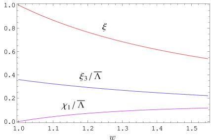
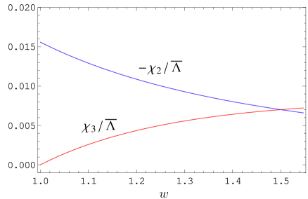
Figure 3: Leading and subleading Isgur-Wise functions for $B_{s}\to D_{s}^{(*)}$ transitions.

The calculated leading and subleading Isgur-Wise functions for $B_{s}\to D_{s}^{(*)}$ transitions are plotted in Fig. 3. Using these Isgur-Wise functions we obtain the decay form factors $h_{i}(w)$ with the account of the first order $1/m_{Q}$ corrections in the whole kinematical range. To improve calculations we scale the results by the values of the form factors at zero recoil $h_{i}(1)$ evaluated with the inclusion of $1/m_{Q}^{2}$ corrections using formulas given in Ref. fg . We find that the account of the first order corrections changes the form factors by about 17%, while the contribution of the second order corrections is less than 3%. These values are in accord with the naive estimates of such corrections $\bar{\Lambda}/(2m_{c})\approx 0.15$ and $[\bar{\Lambda}/(2m_{c})]^{2}\approx 0.02$.

The other popular parametrization for the matrix elements of weak current $J^{W}$ between meson states is given by

$$\langle D_{s}(p_{D_{s}})|\bar{c}\gamma^{\mu}b|B_{s}(p_{B_{s}})\rangle=f_{+}(q^{2})\left[p_{B_{s}}^{\mu}+p_{D_{s}}^{\mu}-\frac{M_{B_{s}}^{2}-M_{D_{s}}^{2}}{q^{2}}\ q^{\mu}\right]+f_{0}(q^{2})\frac{M_{B_{s}}^{2}-M_{D_{s}}^{2}}{q^{2}}\ q^{\mu},$$ (43)

$$\langle D_{s}(p_{D_{s}})|\bar{c}\gamma^{\mu}\gamma_{5}b|B_{s}(p_{B_{s}})\rangle=0,$$ (44)

$$\langle{D^{*}_{s}}(p_{D^{*}_{s}})|\bar{c}\gamma^{\mu}b|B(p_{B_{s}})\rangle = \frac{2iV(q^{2})}{M_{B_{s}}+M_{D^{*}_{s}}}\epsilon^{\mu\nu\rho\sigma}\epsilon^{*}_{\nu}p_{B_{s}\rho}p_{{D^{*}_{s}}\sigma},$$ (45)

$$\langle{D^{*}_{s}}(p_{D^{*}_{s}})|\bar{c}\gamma^{\mu}\gamma_{5}b|B_{s}(p_{B_{s}})\rangle = 2M_{D^{*}_{s}}A_{0}(q^{2})\frac{\epsilon^{*}\cdot q}{q^{2}}\ q^{\mu}+(M_{B_{s}}+M_{D^{*}_{s}})A_{1}(q^{2})\left(\epsilon^{*\mu}-\frac{\epsilon^{*}\cdot q}{q^{2}}\ q^{\mu}\right)$$ (49)

$$-A_{2}(q^{2})\frac{\epsilon^{*}\cdot q}{M_{B_{s}}+M_{D^{*}_{s}}}\left[p_{B_{s}}^{\mu}+p_{D^{*}_{s}}^{\mu}-\frac{M_{B_{s}}^{2}-M_{D^{*}_{s}}^{2}}{q^{2}}\ q^{\mu}\right].$$

At the maximum recoil point ($q^{2}=0$) these form factors satisfy the following conditions:

$$f_{+}(0)=f_{0}(0),$$

$$A_{0}(0)=\frac{M_{B_{s}}+M_{D^{*}_{s}}}{2M_{D^{*}_{s}}}A_{1}(0)-\frac{M_{B_{s}}-M_{D^{*}_{s}}}{2M_{D^{*}_{s}}}A_{2}(0).$$

The relations between two sets of weak decay form factors are given in Appendix B.

Substituting in these relations the Isgur-Wise functions of our model (29)-(33) we find that the decay form factors can be approximated with sufficient accuracy by the following expressions:

(a) $f_{+}(q^{2}),V(q^{2}),A_{0}(q^{2})=F(q^{2})$

$$F(q^{2})=\frac{F(0)}{\displaystyle\left(1-\frac{q^{2}}{M^{2}}\right)\left(1-\sigma_{1}\frac{q^{2}}{M_{B_{c}^{*}}^{2}}+\sigma_{2}\frac{q^{4}}{M_{B_{c}^{*}}^{4}}\right)},$$ (50)

(b) $f_{0}(q^{2}),A_{1}(q^{2}),A_{2}(q^{2})=F(q^{2})$

$$F(q^{2})=\frac{F(0)}{\displaystyle\left(1-\sigma_{1}\frac{q^{2}}{M_{B_{c}^{*}}^{2}}+\sigma_{2}\frac{q^{4}}{M_{B_{c}^{*}}^{4}}\right)},$$ (51)

where $M=M_{B_{c}^{*}}=6.332$ GeV for the form factors $f_{+}(q^{2}),V(q^{2})$ and $M=M_{B_{c}}=6.272$ GeV for the form factor $A_{0}(q^{2})$; the values $F(0)$ and $\sigma_{1,2}$ are given in Table 1. The values of $\sigma_{1,2}$ are determined with a few tenths of percent errors. The main uncertainties of the form factors originate from the account of $1/m_{Q}^{2}$ corrections at zero recoil only and from the higher order $1/m_{Q}^{3}$ contributions and can be roughly estimated in our approach to be about 2%.  The $q^{2}$ dependence of these form factors is shown in Fig. 4.

Table 1: Form factors of weak $B_{s}\to D_{s}^{(*)}$ transitions calculated in our model. Form factors $f_{+}(q^{2})$, $V(q^{2})$, $A_{0}(q^{2})$ are fitted by Eq. (50), and form factors $f_{0}(q^{2})$, $A_{1}(q^{2})$, $A_{2}(q^{2})$ are fitted by Eq. (51).

	$B_{s}\to D_{s}$		$B_{s}\to D^{*}_{s}$
	$f_{+}$	$f_{0}$	$V$	$A_{0}$	$A_{1}$	$A_{2}$
$F(0)$	0.74	0.74	0.95	0.67	0.70	0.75
$F(q^{2}_{\rm max})$	1.15	0.88	1.50	1.06	0.84	1.04
$\sigma_{1}$	0.200	0.430	0.372	0.350	0.463	1.04
$\sigma_{2}$	$-0.461$	$-0.464$	$-0.561$	$-0.600$	$-0.510$	$-0.070$

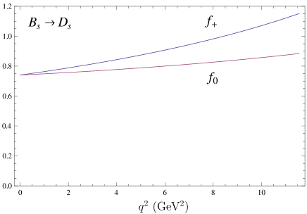
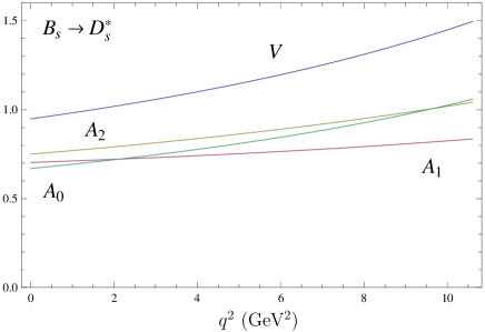
Figure 4: Form factors of weak $B_{s}\to D_{s}^{(*)}$ transitions.

Table 2: Comparison of theoretical predictions for the form factors of semileptonic decays $B_{s}\to D_{s}^{(*)}e\nu$ at maximum recoil point $q^{2}=0$.

	$f_{+}(0)$	$V(0)$	$A_{0}(0)$	$A_{1}(0)$	$A_{2}(0)$
this paper	$0.74\pm 0.02$	$0.95\pm 0.02$	$0.67\pm 0.01$	$0.70\pm 0.01$	$0.75\pm 0.02$
kp	0.61	0.64		0.56	0.59
bcnp	$0.7\pm 0.1$	$0.63\pm 0.05$	$0.52\pm 0.06$	$0.62\pm 0.01$	$0.75\pm 0.07$
cfkw	$0.57^{+0.02}_{-0.03}$	$0.70^{+0.05}_{-0.04}$		$0.65^{+0.01}_{-0.01}$	$0.67^{+0.01}_{-0.01}$
llw	$0.86^{+0.17}_{-0.15}$
lsw		$0.74^{+0.05}_{-0.05}$	$0.63^{+0.04}_{-0.04}$	$0.61^{+0.04}_{-0.04}$	$0.59^{+0.04}_{-0.04}$

In Table 2 we confront our predictions for the form factors of semileptonic decays $B_{s}\to D_{s}^{(*)}e\nu$ at maximum recoil point $q^{2}=0$ with results of other approaches kp ; bcnp ; cfkw ; llw ; lsw . Different quark models are used in Refs. kp ; cfkw ; lsw , while the QCD and light cone sum rules are employed in Refs. bcnp ; llw . We find that these significantly different theoretical calculations lead to rather close values of the decay form factors. One of the main advantages of our model is its ability not only to obtain the decay form factors at the single kinematical point, but also to determine its $q^{2}$ dependence in the whole range without any additional assumptions or extrapolations.

V Semileptonic $B_{s}$ decays to $D_{s}$ mesons

The differential decay rate for the semileptonic $B_{s}$ meson decay to $D_{s}^{(*)}$ mesons reads iks

$$\frac{d\Gamma(B_{s}\to D_{s}^{(*)}l\bar{\nu})}{dq^{2}}=\frac{G_{F}^{2}}{(2\pi)^{3}}|V_{cb}|^{2}\frac{\lambda^{1/2}(q^{2}-m_{l}^{2})^{2}}{24M_{B_{s}}^{3}q^{2}}\Biggl{[}HH^{{\dagger}}\left(1+\frac{m_{l}^{2}}{2q^{2}}\right)+\frac{3m_{l}^{2}}{2q^{2}}H_{t}H^{{\dagger}}_{t}\Biggr{]},$$ (52)

where $G_{F}$ is the Fermi constant, $V_{cb}$ is the CKM matrix element, $\lambda\equiv\lambda(M_{B_{s}}^{2},M_{D_{s}^{(*)}}^{2},q^{2})=M_{B_{s}}^{4}+M_{D_{s}^{(*)}}^{4}+q^{4}-2(M_{B_{s}}^{2}M_{D_{s}^{(*)}}^{2}+M_{D_{s}^{(*)}}^{2}q^{2}+M_{B_{s}}^{2}q^{2})$, $m_{l}$ is the lepton mass and

$$HH^{{\dagger}}\equiv H_{+}H^{{\dagger}}_{+}+H_{-}H^{{\dagger}}_{-}+H_{0}H^{{\dagger}}_{0}.$$ (53)

The helicity components $H_{\pm}$, $H_{0}$ and $H_{t}$ of the hadronic tensor are expressed through the invariant form factors. They are given in Appendix C.

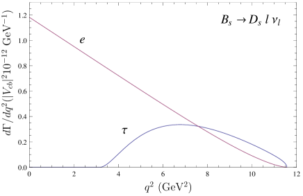
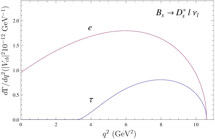
Figure 5: Predictions for the differential decay rates of the $B_{s}\to D_{s}^{(*)}l\nu$ semileptonic decays.

Now we substitute the weak decay form factors calculated in the previous section into the above expressions for decay rates. The resulting differential decay rates for the $B_{s}$ decays to the $D_{s}^{(*)}$ mesons are plotted in Fig. 5. The corresponding total decay rates are obtained by integrating the differential decay rates over $q^{2}$. For calculations we use the CKM matrix element $|V_{cb}|=(3.9\pm 0.15)\times 10^{-2}$, which was obtained from the comparison of our theoretical predictions hlsem ; fgtau for the products $F_{D^{(*)}}(w)|V_{cb}|$ and for the $B\to D^{(*)}l\nu_{l}$ decay branching fractions with updated experimental data.  It is necessary to point out that the kinematical range accessible in these semileptonic decays is rather broad. Therefore the knowledge of the $q^{2}$ dependence of the form factors is very important for reducing theoretical uncertainties of the decay rates. Our results for the semileptonic $B_{s}\to D_{s}^{(*)}l\nu$ decay rates are given in Table 3 in comparison with previous calculations. The authors of Ref.bcnp use the QCD sum rules, while the light cone sum rules approach is adopted in Ref. llw . Different types of constituent quark models are employed in Refs. lsw ; cfkw ; zll and the three point QCD sum rules are used in Ref. ab . We see that our predictions are consistent with results of quark model calculations in Refs. lsw ; cfkw . They are approximately two times larger than the QCD sum rules and light cone sum rules results of Refs. bcnp ; llw , but slightly lower than the values of Refs. zll ; ab .

We find that the total branching fraction of the semileptonic decays of $B_{s}$ mesons to the ground state $D_{s}^{(*)}$ is equal to $Br(B_{s}\to D_{s}^{(*)}e\nu)=(7.4\pm 0.7)\%$ and $Br(B_{s}\to D_{s}^{(*)}\tau\nu)=(1.92\pm 0.15)\%$. The errors in our estimates originate from the uncertainties in the determination of the CKM matrix element $|V_{cb}|$, which are dominant, and from the theoretical uncertainties in the determination of decay form factors. The latter uncertainties are considerably smaller than the former ones and are mostly related with the estimates of the higher order terms in the heavy quark expansion.

Table 3: Comparison of theoretical predictions for the branching fractions of semileptonic decays $B_{s}\to D_{s}^{(*)}l\nu$ (in %).

Decay	this paper	bcnp	cfkw	llw	lsw	zll	ab
$B_{s}\to D_{s}e\nu$	$2.1\pm 0.2$	$1.35\pm 0.21$	1.4-1.7	$1.0^{+0.4}_{-0.3}$		2.73-3.00	2.8-3.8
$B_{s}\to D_{s}\tau\nu$	$0.62\pm 0.05$		0.47-0.55	$0.33^{+0.14}_{-0.11}$
$B_{s}\to D_{s}^{*}e\nu$	$5.3\pm 0.5$	$2.5\pm 0.1$	5.1-5.8		$5.2\pm 0.6$	7.49-7.66	1.89-6.61
$B_{s}\to D_{s}^{*}\tau\nu$	$1.3\pm 0.1$		1.2-1.3		$1.3^{+0.2}_{-0.1}$

VI Form factors of weak $B_{s}$ decays to radially excited $D_{s}(2S)$ mesons

The decay form factors (20)-(26) up to $1/m_{Q}$ order in HQET for $B_{s}$ decays to radially excited $D_{s}[(n+1)S]$ mesons are expressed through one leading $\xi^{(n)}$ and five subleading $\tilde{\xi}_{3}$, $\tilde{\chi}_{1,2,3,b}$ Isgur-Wise functions and two mass parameters $\bar{\Lambda}$ and $\bar{\Lambda}^{(n)}$ radexc . They are presented in Appendix D.

In our model all HQET relations (135)-(151) are satisfied and we get the following expressions for the leading and subleading Isgur-Wise functions radexc :

$$\xi^{(1)}(w) = \left(\frac{2}{w+1}\right)^{1/2}\int\frac{d^{3}p}{(2\pi)^{3}}\bar{\psi}^{(0)}_{D_{s}(2S)}\!\!\left({\bf p}+2\epsilon_{s}(p)\sqrt{\frac{w-1}{w+1}}{\bf e_{\Delta}}\right)\psi^{(0)}_{B_{s}}({\bf p}),$$ (54)

$$\tilde{\xi}_{3}(w) = \left(\frac{\bar{\Lambda}^{(1)}+\bar{\Lambda}}{2}-m_{s}+\frac{1}{6}\frac{\bar{\Lambda}^{(1)}-\bar{\Lambda}}{w-1}\right)\left(1+\frac{2}{3}\frac{w-1}{w+1}\right)\xi^{(1)}(w),$$ (57)

$$\tilde{\chi}_{1}(w) \cong \frac{1}{20}\frac{w-1}{w+1}\frac{\bar{\Lambda}^{(1)}-\bar{\Lambda}}{w-1}\xi^{(1)}(w)$$ (61)

$$+\frac{\bar{\Lambda}^{(1)}}{2}\left(\frac{2}{w+1}\right)^{1/2}\int\frac{d^{3}p}{(2\pi)^{3}}\bar{\psi}^{(1)si}_{D_{s}(2S)}\!\!\left({\bf p}+2\epsilon_{s}(p)\sqrt{\frac{w-1}{w+1}}{\bf e_{\Delta}}\right)\psi^{(0)}_{B_{s}}({\bf p}),$$

$$\tilde{\chi}_{2}(w) \cong -\frac{1}{12}\frac{1}{w+1}\frac{\bar{\Lambda}^{(1)}-\bar{\Lambda}}{w-1}\xi^{(1)}(w),$$ (63)

$$\tilde{\chi}_{3}(w) \cong -\frac{3}{80}\frac{w-1}{w+1}\frac{\bar{\Lambda}^{(1)}-\bar{\Lambda}}{w-1}\xi^{(1)}(w)$$ (67)

$$+\frac{\bar{\Lambda}^{(1)}}{4}\left(\frac{2}{w+1}\right)^{1/2}\int\frac{d^{3}p}{(2\pi)^{3}}\bar{\psi}^{(1)sd}_{D_{s}(2S)}\!\!\left({\bf p}+2\epsilon_{s}(p)\sqrt{\frac{w-1}{w+1}}{\bf e_{\Delta}}\right)\psi^{(0)}_{B_{s}}({\bf p}),$$

$$\chi_{b}(w)\!\! \cong \!\!\bar{\Lambda}\left(\frac{2}{w+1}\right)^{1/2}\!\int\frac{d^{3}p}{(2\pi)^{3}}\bar{\psi}^{(0)}_{D_{s}(2S)}\!\!\left({\bf p}+2\epsilon_{s}(p)\sqrt{\frac{w-1}{w+1}}{\bf e_{\Delta}}\right)\left[\psi^{(1)si}_{B_{s}}({\bf p})-3\psi^{(1)sd}_{B_{s}}({\bf p})\right],\ \ \ \ \ \$$ (69)

where ${\bf\Delta}^{2}=M_{D_{s}^{(*)}(2S)}^{2}(w^{2}-1)$. Here we used the expansion for the $S$-wave meson wave function radexc

$$\psi_{M}=\psi_{M}^{(0)}+\bar{\Lambda}_{M}\varepsilon_{Q}\left(\psi_{M}^{(1)si}+d_{M}\psi_{M}^{(1)sd}\right)+O(1/m_{Q}^{2}),$$

where $\psi_{M}^{(0)}$ is the wave function in the limit $m_{Q}\to\infty$, $\psi_{M}^{(1)si}$ and $\psi_{M}^{(1)sd}$ are the spin-independent and spin-dependent first order $1/m_{Q}$ corrections, $d_{P}=-3$ for pseudoscalar and $d_{V}=1$ for vector mesons. The symbol $\cong$ in the expressions (61)–(69) for the subleading functions $\tilde{\chi}_{i}(w)$ implies that corrections suppressed by an additional power of the ratio $(w-1)/(w+1)$, which is equal to zero at $w=1$ and less than $1/6$ at $w_{\rm max}$, were neglected. Since the main contribution to the decay rate comes from the values of form factors close to $w=1$, these corrections turn out to be unimportant.

It is clear from the expression (54) that the leading order contribution vanishes at the point of zero recoil (${\bf\Delta}=0,w=1$) of the final $D_{s}^{(*)}(2S)$ meson, since the radial parts of the wave functions $\Psi_{D_{s}(2S)}$ and $\Psi_{B_{s}}$ are orthogonal in the infinitely heavy quark limit.

Near the zero recoil point of the final meson $w=1$ the Isgur-Wise functions have the following expansions

$$\xi^{(1)}(w) = 2.455(w-1)-9.545(w-1)^{2}+\cdots,$$ (70)

$$\tilde{\xi}_{3}(w)/\tilde{\Lambda} = 0.221+1.094(w-1)-5.294(w-1)^{2}+\cdots,$$ (72)

$$\tilde{\chi}_{1}(w)/\tilde{\Lambda} = 0.182-0.143(w-1)-1.055(w-1)^{2}+\cdots,$$ (74)

$$\tilde{\chi}_{2}(w)/\tilde{\Lambda} = -0.0552+0.242(w-1)-0.547(w-1)^{2}+\cdots,$$ (76)

$$\tilde{\chi}_{3}(w)/\tilde{\Lambda} = -0.00133-0.0334(w-1)+0.150(w-1)^{2}+\cdots,$$ (78)

$$\tilde{\chi}_{b}(w)/\tilde{\Lambda} = -0.169+1.114(w-1)-4.060(w-1)^{2}+\cdots,$$ (80)

where $\tilde{\Lambda}=(\bar{\Lambda}^{(1)}+\bar{\Lambda})/2$.

The leading $\xi^{(1)}$ and subleading $\tilde{\xi}_{3}$, $\tilde{\chi}_{1,2,3,b}$ Isgur-Wise functions for $B_{s}\to D_{s}^{(*)}(2S)$ transitions are shown in Fig. 6. We use relations (117)-(128) to express form factors $f_{+,0}(q^{2})$, $V(q^{2})$ and $A_{0,1,2}$ through the calculated Isgur-Wise functions. The obtained form factors are plotted in Fig. 7. Their values at zero and maximum $q^{2}$ are given in Table 4. The main theoretical uncertainties of the decay from factors, as for the decays to the ground state mesons, originate from the higher order $1/m_{Q}$ contributions and are less than 4%. Comparing plots in Figs. 4 and 7 we see that form factors for the decays to ground and radially excited states have significantly different behaviour in $q^{2}$. The former ones grow with $q^{2}$, while the latter ones decrease. This is the consequence of the different structure of nodes of the wave functions of these states.

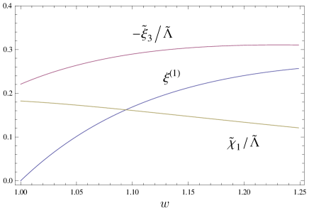
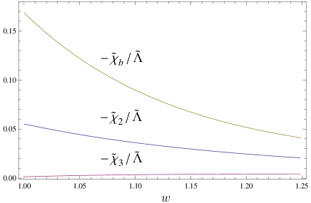
Figure 6: Leading and subleading Isgur-Wise functions for $B_{s}\to D_{s}^{(*)}(2S)$ transitions ($\tilde{\Lambda}=(\bar{\Lambda}^{(1)}+\bar{\Lambda})/2$).

Table 4: Form factors of weak $B_{s}\to D_{s}^{(*)}(2S)$ transitions calculated in our model.

	$B_{s}\to D_{s}(2S)$		$B_{s}\to D^{*}_{s}(2S)$
	$f_{+}$	$f_{0}$	$V$	$A_{0}$	$A_{1}$	$A_{2}$
$F(0)$	0.41	0.41	0.46	0.45	0.32	0.058
$F(q^{2}_{\rm max})$	0.28	0.075	0.28	0.29	0.072	$-0.29$

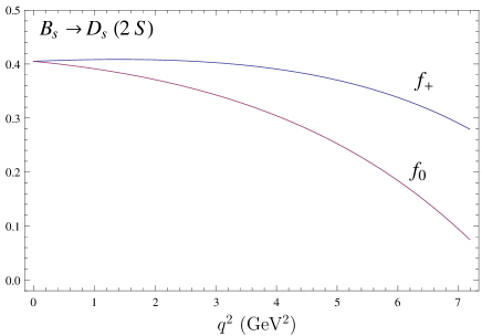
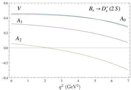
Figure 7: Form factors of the weak $B_{s}\to D_{s}^{(*)}(2S)$ transitions.

VII Semileptonic $B_{s}$ decays to radially excited $D_{s}(2S)$ mesons

For the calculation of the semileptonic $B_{s}$ decays to radially excited $D_{s}(2S)$ mesons we use the expression for the differential decay rates (52) with the helicity components of the hadronic tensor given by Eqs. (129)-(134) and decay form factors calculated in the previous section. The predictions for the corresponding branching fractions are given in Table 5. We find that semileptonic $B_{s}$ decays to the pseudoscalar $D_{s}(2S)$ and vector $D_{s}^{*}(2S)$ mesons have close values. The total contribution of these decays is obtained to be $Br(B_{s}\to D_{s}^{(*)}(2S)e\nu)=(0.65\pm 0.06)\%$ and $Br(B_{s}\to D_{s}^{(*)}(2S)\tau\nu)=(0.026\pm 0.003)\%$.

Table 5: Predictions for the branching fractions of semileptonic decays $B_{s}\to D_{s}^{(*)}(2S)l\nu$ (in %).

Decay	Br
$B_{s}\to D_{s}(2S)e\nu$	$0.27\pm 0.03$
$B_{s}\to D_{s}(2S)\tau\nu$	$0.011\pm 0.001$
$B_{s}\to D_{s}^{*}(2S)e\nu$	$0.38\pm 0.04$
$B_{s}\to D_{s}^{*}(2S)\tau\nu$	$0.015\pm 0.002$

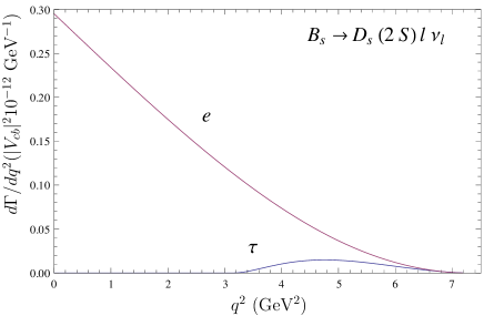
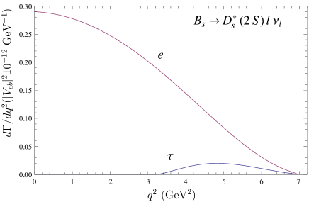
Figure 8: Predictions for the differential decay rates of the $B_{s}\to D_{s}^{(*)}(2S)l\nu$ semileptonic decays.

The differential decay rates of the $B_{s}\to D_{s}^{(*)}(2S)l\nu$ semileptonic decays are plotted in Fig 8.

VIII Form factors of weak $B_{s}$ decays to orbitally excited $D_{sJ}^{(*)}$ mesons

The matrix elements of the weak current $J^{W}_{\mu}=\bar{b}\gamma_{\mu}(1-\gamma_{5})c$ for $B_{s}$ decays to orbitally excited scalar $D_{s0}^{*}$ mesons can be parametrized by two invariant form factors

$$\langle D_{s0}^{*}(p_{D_{s0}})|\bar{c}\gamma^{\mu}b|B_{s}(p_{B_{s}})\rangle = 0,$$ (81)

$$\langle D_{s0}^{*}(p_{D_{s0}})|\bar{c}\gamma^{\mu}\gamma_{5}b|B(p_{B_{s}})\rangle = r_{+}(q^{2})\left(p_{B_{s}}^{\mu}+p_{D_{s0}}^{\mu}\right)+r_{-}(q^{2})\left(p_{B_{s}}^{\mu}-p_{D_{s0}}^{\mu}\right),$$ (83)

where $q=p_{B_{s}}-p_{D_{s0}}$, $M_{D_{s0}}$ is the scalar meson mass.

The matrix elements of the weak current for $B_{s}$ decays to the axial vector $D_{s1}$ meson can be expressed in terms of four invariant form factors

$$\langle D_{s1}(p_{D_{s1}})|\bar{c}\gamma^{\mu}b|B(p_{B_{s}})\rangle\!\! = \!\!(M_{B_{s}}+M_{D_{s1}})h_{V_{1}}(q^{2})\epsilon^{*\mu}+[h_{V_{2}}(q^{2})p_{B_{s}}^{\mu}+h_{V_{3}}(q^{2})p_{D_{s1}}^{\mu}]\frac{\epsilon^{*}\cdot q}{M_{B_{s}}},\qquad$$ (84)

$$\langle D_{s1}(p_{D_{s1}})|\bar{c}\gamma^{\mu}\gamma_{5}b|B(p_{B_{s}})\rangle\!\! = \!\!\frac{2ih_{A}(q^{2})}{M_{B_{s}}+M_{D_{s1}}}\epsilon^{\mu\nu\rho\sigma}\epsilon^{*}_{\nu}p_{B_{s}\rho}p_{{D_{s1}}\sigma},$$ (86)

where $M_{D_{s1}}$ and $\epsilon^{\mu}$ are the mass and polarization vector of the axial vector meson. The matrix elements of the weak current for $B_{s}$ decays to the axial vector $D_{s1}^{\prime}$ meson are obtained from Eqs. (84) by the replacement of the set of form factors $h_{i}(q^{2})$ by $g_{i}(q^{2})$ ($i=V_{1},V_{2},V_{3},A$).

The matrix elements of the weak current for $B_{s}$ decays to the tensor $D_{s2}^{*}$ meson can be decomposed in four Lorentz-invariant structures

$$\langle D_{s2}^{*}(p_{D_{s2}})|\bar{c}\gamma^{\mu}b|B(p_{B_{s}})\rangle = \frac{2it_{V}(q^{2})}{M_{B_{s}}+M_{D_{s2}}}\epsilon^{\mu\nu\rho\sigma}\epsilon^{*}_{\nu\alpha}\frac{p_{B_{s}}^{\alpha}}{M_{B_{s}}}p_{B_{s}\rho}p_{{D_{s2}}\sigma},$$ (87)

$$\langle D_{s2}^{*}(p_{D_{s2}})|\bar{q}\gamma^{\mu}\gamma_{5}b|B(p_{B_{s}})\rangle = (M_{B_{s}}+M_{D_{s2}})t_{A_{1}}(q^{2})\epsilon^{*\mu\alpha}\frac{p_{B_{s}\alpha}}{M_{B_{s}}}$$ (91)

$$+[t_{A_{2}}(q^{2})p_{B_{s}}^{\mu}+t_{A_{3}}(q^{2})p_{D_{s2}}^{\mu}]\epsilon^{*}_{\alpha\beta}\frac{p_{B_{s}}^{\alpha}p_{B_{s}}^{\beta}}{M_{B_{s}}^{2}},$$

where $M_{D_{s2}}$ and $\epsilon^{\mu\nu}$ are the mass and polarization tensor of the tensor meson.

To obtain the form factors of $B_{s}\to D_{sJ}^{(*)}$ weak transitions we use the expression for the weak current matrix element (11). We calculate exactly the contribution of the leading vertex function $\Gamma^{(1)}({\bf p},{\bf q})$ (12) to the transition matrix element of the weak current (11) using the $\delta$-function. For the evaluation of the subleading contribution $\Gamma^{(2)}({\bf p},{\bf q})$ for the $B\to D_{sJ}^{(*)}$ transitions, governed by the heavy-to-heavy $b\to c$ transitions, we use expansions in inverse powers of masses of the heavy $b$- and $c$-quarks, contained in the initial $B_{s}$ meson and final $D_{sJ}^{(*)}$ meson. Thus we can neglect the small relative quark momentum $|{\bf p}|$ compared to the heavy quark mass $m_{Q}$ in the quark energy $\epsilon_{Q}(p+\Delta)\equiv\sqrt{m_{Q}^{2}+({\bf p}+{\bf\Delta})^{2}}$, replacing it by $\epsilon_{Q}(\Delta)\equiv\sqrt{m_{Q}^{2}+{\bf\Delta}^{2}}$ in expressions for the $\Gamma^{(2)}({\bf p},{\bf q})$. Note that we keep the dependence on the recoil momentum ${\bf\Delta}={\bf p}_{D_{sJ}^{(*)}}-{\bf p}_{B_{s}}$. This replacement removes the relative momentum dependence in the quark energy and thus permits us to perform one of the integrations in the $\Gamma^{(2)}_{\mu}({\bf p},{\bf q})$ contribution using the quasipotential equation. The subleading contribution turns out to be rather small numerically, since it is proportional to the quark binding energy in the meson. Therefore we obtain reliable expressions for the form factors in the whole accessible kinematical range. It is important to emphasize that when doing these calculations we consistently take into account all relativistic contributions including boosts of the meson wave functions from the rest reference frame to the moving ones, given by Eq. (18). The obtained expressions for the decay form factors are rather cumbersome and are given in the Appendix of Ref. bcexc . Note that, while calculating form factors of weak $B_{s}$ decays to $D_{s1}$ and $D^{\prime}_{s1}$ mesons, it is important to take into account the mixing (16) of singlet $D_{s}(^{1}P_{1})$ and triplet $D_{s}(^{3}P_{1})$ states.

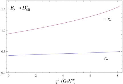
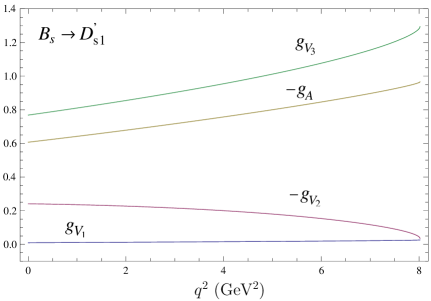
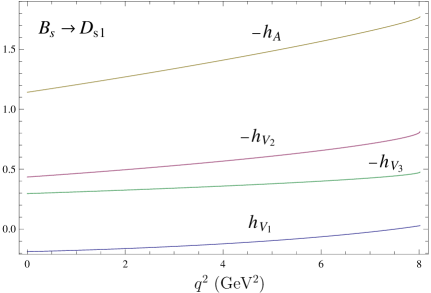
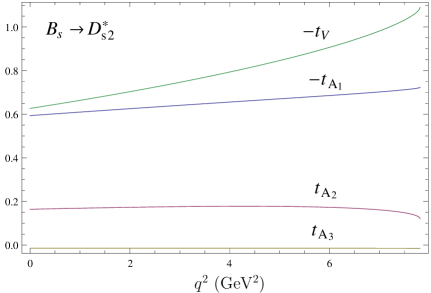
Figure 9: Form factors of the $B_{s}$ decays to the $P$–wave $D_{sJ}^{(*)}$ mesons.

Table 6: Calculated values of the form factors of the $B_{s}$ decays to the $P$–wave $D_{sJ}^{(*)}$ at $q^{2}=0$ and $q^{2}=q^{2}_{\rm max}\equiv(M_{B_{s}}-M_{D_{sJ}})^{2}$.

	$B_{s}\to D_{s0}^{*}$		$B_{s}\to D_{s1}^{\prime}$				$B_{s}\to D_{s1}$				$B_{s}\to D_{s2}^{*}$
$q^{2}$	$r_{+}$	$r_{-}$	$g_{A}$	$g_{V_{1}}$	$g_{V_{2}}$	$g_{V_{3}}$	$h_{A}$	$h_{V_{1}}$	$h_{V_{2}}$	$h_{V_{3}}$	$t_{V}$	$t_{A_{1}}$	$t_{A_{2}}$	$t_{A_{3}}$
0	0.40	$-0.91$	$-0.61$	$0.01$	$-0.24$	0.77	$-1.14$	$-0.19$	$-0.43$	$-0.29$	$-0.63$	$-0.59$	$0.16$	$-0.01$
$q^{2}_{\rm max}$	0.50	$-1.58$	$-0.97$	0.03	$-0.04$	$1.29$	$-1.77$	$0.03$	$-0.81$	$-0.48$	$-1.09$	$-0.72$	$0.12$	$-0.02$

In Fig. 9 we plot form factors of the weak $B_{s}$ transitions to the $P$-wave $D_{sJ}^{(*)}$ mesons. The calculated values of these form factors at $q^{2}=0$ and $q^{2}=q^{2}_{\rm max}\equiv(M_{B_{s}}-M_{D_{sJ}})^{2}$ are displayed in Table 6. The theoretical uncertainties of these form factors within our approach are mainly determined by the errors introduced by the replacement of $\epsilon_{c}(p+\Delta)$ by $\epsilon_{c}(\Delta)$ in the subleading vertex $\Gamma^{(2)}({\bf p},{\bf q})$ and $O(1/m_{b}^{3})$ contributions. They are almost negligible at $q^{2}=0$ and are less than 1% at $q^{2}=q^{2}_{\rm max}$.

IX Semileptonic $B_{s}$ decays to orbitally excited $D_{sJ}^{(*)}$ mesons

The differential semileptonic decay rates of $B_{s}$ mesons to orbitally excited $D_{sJ}^{(*)}$ mesons are given by Eq. (52). The helicity components $H_{\pm}$, $H_{0}$ and $H_{t}$ of the hadronic tensor are expressed through the invariant form factors (81)-(91) by the relations bcexc given in Appendix E.

Table 7: Comparison of the predictions for the branching fractions of the semileptonic decays $B_{s}\to D_{sJ}^{(*)}l\nu$ (in %).

Decay	this paper	$m\to\infty$	with $1/m_{Q}$	saefhp	zll	llw	as	h
		orbexc	orbexc
$B_{s}\to D_{s0}^{*}e\nu$	$0.36\pm 0.04$	0.10	0.37	0.443	0.49-0.571	$0.23^{+0.12}_{-0.10}$	$\sim 0.1$	0.20
$B_{s}\to D_{s0}^{*}\tau\nu$	$0.019\pm 0.002$					$0.057^{+0.028}_{-0.023}$	$\sim 0.01$
$B_{s}\to D_{s1}^{\prime}e\nu$	$0.19\pm 0.02$	0.13	0.18	0.174-0.570	0.752-0.869		$0.49$	0.10
$B_{s}\to D_{s1}^{\prime}\tau\nu$	$0.015\pm 0.002$
$B_{s}\to D_{s1}e\nu$	$0.84\pm 0.09$	0.36	1.06	0.477
$B_{s}\to D_{s1}\tau\nu$	$0.049\pm 0.005$
$B_{s}\to D_{s2}^{*}e\nu$	$0.67\pm 0.07$	0.56	0.75	0.376
$B_{s}\to D_{s2}^{*}\tau\nu$	$0.029\pm 0.003$

Substituting calculated form factors in these expressions we get predictions for the branching fractions of the semileptonic $B_{s}$ decays to orbitally excited $D_{s}$ mesons. We find that decays to $D_{s1}$ and $D^{*}_{s2}$ mesons are dominant. The obtained results are given in Table 7 in comparison with other calculations. First we compare with our previous calculation orbexc which was performed in the framework of the heavy quark expansion. We give results found in the infinitely heavy quark limit ($m_{Q}\to\infty$) and with the account of first order $1/m_{Q}$ corrections. It was argued orbexc ; llsw that $1/m_{Q}$ corrections are large and their inclusion significantly influences the decays rates. The large effect of subleading heavy quark corrections was found to be a consequence of the vanishing of the leading order contributions to the decay matrix elements, due to heavy quark spin-flavour symmetry, at the point of zero recoil of the final charmed meson, while the subleading order contributions do not vanish at this kinematical point. Here we calculated the decay rates without application of the heavy quark expansion. We find that nonperturbative results agree well with the ones obtained with the account of the leading order $1/m_{Q}$ corrections orbexc . This means that the higher order in $1/m_{Q}$ corrections are small, as was expected. Then we compare our predictions with the results of calculations in other approaches. The authors of Refs. saefhp ; zll employ different types of constituent quark models for their calculations. Light cone and three point QCD sum rules are used in Refs. llw ; as , while HQET and sum rules are applied in Ref. h . In general we find reasonable agreement between our predictions and results of Refs. saefhp ; llw ; as ; h , but results of the quark model calculations zll are slightly larger.

In Fig. 10 we plot the differential decay rates of the $B\to D_{sJ}^{(*)}l\nu$ semileptonic decays. The total semileptonic decay branching fractions to orbitally excited $D_{s}$ mesons are found to be $Br(B_{s}\to D_{sJ}^{(*)}e\nu)=(2.1\pm 0.2)\%$ and $Br(B_{s}\to D_{sJ}^{(*)}\tau\nu)=(0.11\pm 0.01)\%$.

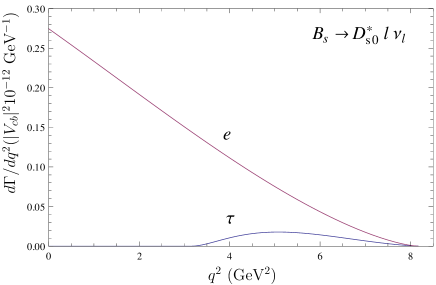
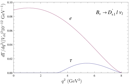
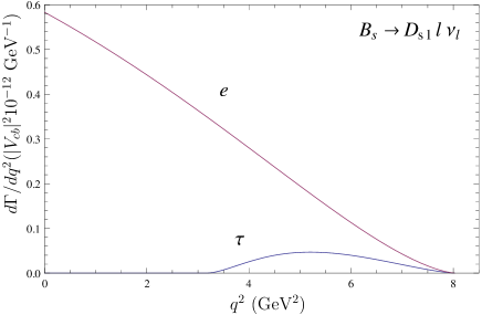
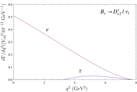
Figure 10: Predictions for the differential decay rates of the $B\to D_{sJ}^{(*)}l\nu$ semileptonic decays.

The first experimental measurement of the semileptonic decay $B_{s}\to D_{s1}\mu\nu$ was done by the D0 Collaboration d0 . The branching fraction was obtained by assuming that the $D_{s1}$ production in semileptonic decay comes entirely from the $B_{s}$ decay and using a prediction for $Br(D_{s1}\to D^{*}K^{0}_{S})=0.25$. Its value

$$Br(B_{s}\to D_{s1}X\mu\nu)_{\rm D0}=(1.03\pm 0.20\pm 0.17\pm 0.14)\%$$

is in good agreement with our prediction $0.84\pm 0.9$ given in Table 7.

Recently the LHCb Collaboration lhcb3 reported the first observation of the orbitally excited $D_{s2}^{*}$ meson in the semileptonic $B_{s}$ decays. The decay to the $D_{s1}$ meson was also observed. The measured branching fractions relative to the total $B_{s}$ semileptonic rate are

$$Br(B_{s}\to D_{s2}^{*}X\mu\nu)/Br(B_{s}\to X\mu\nu)_{\rm LHCb}=(3.3\pm 1.0\pm 0.4)\%,$$

$$Br(B_{s}\to D_{s1}X\mu\nu)/Br(B_{s}\to X\mu\nu)_{\rm LHCb}=(5.4\pm 1.2\pm 0.5)\%.$$

The $D_{s2}^{*}/D_{s1}$ event ratio is found to be

$$Br(B_{s}\to D_{s2}^{*}X\mu\nu)/Br(B_{s}\to D_{s1}X\mu\nu)_{\rm LHCb}=0.61\pm 0.14\pm 0.05.$$

These values can be compared with our predictions if we assume that decays to $D_{s1}$ and $D_{s2}^{*}$ mesons give dominant contributions to the ratios. Summing up the semileptonic $B_{s}$ decay branching fractions to ground state, first radial and orbital excitations of $D_{s}$ mesons, presented in Secs. V, VII, IX, we get for the total $B_{s}$ semileptonic rate $Br(B_{s}\to X\mu\nu)=(10.2\pm 1.0)\%$. Then using the calculated values from Table 7 we get

$$Br(B_{s}\to D_{s2}^{*}\mu\nu)/Br(B_{s}\to X\mu\nu)_{\rm theor}=(6.5\pm 1.2)\%,$$

$$Br(B_{s}\to D_{s1}\mu\nu)/Br(B_{s}\to X\mu\nu)_{\rm theor}=(8.2\pm 1.6)\%,$$

and

$$Br(B_{s}\to D_{s2}^{*}\mu\nu)/Br(B_{s}\to D_{s1}\mu\nu)_{\rm theor}=0.79\pm 0.14.$$

The predicted central values are larger than experimental ones, but the results agree with experiment within $2\sigma$.

X Nonleptonic decays

In the standard model nonleptonic $B_{s}$ decays are described by the effective Hamiltonian, obtained by integrating out the $W$-boson and top quark. For the nonleptonic $B_{s}$ decay to the ground state or excited $D_{s}$ meson and light meson governed by $b\to c$ transition the effective Hamiltonian is given by bbl

$$H_{\rm eff}=\frac{G_{F}}{\sqrt{2}}V_{cb}^{*}V_{uq}\left[c_{1}(\mu)O_{1}^{u}+c_{2}(\mu)O_{2}^{u}\right],$$ (92)

where $q=d,s$. For the nonleptonic $B_{s}$ decay to two charmed mesons the effective Hamiltonian ($\Delta B=1$) bbl reads

$$H_{\rm eff}=\frac{G_{F}}{\sqrt{2}}V_{cb}^{*}V_{cq}\sum_{i=1}^{10}c_{i}(\mu)O_{i}^{c}.$$ (93)

The Wilson coefficients $c_{i}(\mu)$ are evaluated perturbatively at the $W$ scale and then are evolved down to the renormalization scale $\mu\approx m_{b}$ by the renormalization-group equations. Functions $O_{i}^{q^{\prime}}$ are the local four-quark operators. The tree level operators have the form

$$O_{1}^{q^{\prime}} = (\bar{b}c)_{V-A}(\bar{q}^{\prime}q)_{V-A},$$ (94)

$$O_{2}^{q^{\prime}} = (\bar{b}_{j}c_{i})_{V-A}(\bar{q}^{\prime}_{j}q_{i})_{V-A},\$$ (95)

while the functions $O_{i}$ ($i=3,..,10$) are the penguin operators. The following notations are used

$$(\bar{q}q^{\prime})_{V\mp A}=\bar{q}\gamma_{\mu}(1\mp\gamma_{5})q^{\prime}.$$

The amplitude of the nonleptonic two-body $B_{s}$ decay to $D_{s}$ and light $M$ mesons can be expressed through the matrix element of the effective weak Hamiltonian $H_{\rm eff}$ in the following way

$$M(B_{s}\to D_{s}M)=\langle D_{s}M|H_{\rm eff}|B_{s}\rangle=\frac{G_{F}}{\sqrt{2}}\Biggl{\{}V_{cb}^{*}V_{uq}\left[c_{1}\langle D_{s}M|O_{1}^{u}|B_{s}\rangle+c_{2}\langle D_{s}M|O_{2}^{u}|B_{s}\rangle\right]\Biggr{\}}.$$ (96)

The factorization approach, which is widely used for the calculation of two-body nonleptonic decays, such as $B_{s}\to D_{s}M$, assumes that the nonleptonic decay amplitude reduces to the product of a meson transition matrix element and a weak decay constant bsw . Clearly, this assumption is not exact. However, it is expected that factorization can hold for energetic decays, where one final meson is heavy and the other meson is light and energetic dg . A more general treatment of factorization is given in Ref. bbns .

Then the $B_{s}\to D_{s}^{-}M^{+}$ decay amplitude can be approximated by the product of one-particle matrix elements. The matrix element $(q=d,s)$ is given by

$$\langle M^{+}D_{s}^{-}|c_{1}O_{1}^{u}+c_{2}O_{2}^{u}|B_{s}^{0}\rangle\approx a_{1}\langle D_{s}^{-}|(\bar{b}c)_{V-A}|B_{s}^{0}\rangle\langle M^{+}|(\bar{u}q)_{V-A}|0\rangle,$$ (97)

where the Wilson coefficients appear in the following linear combination

$$a_{1}=c_{1}+\frac{1}{N_{c}}c_{2}$$ (98)

and $N_{c}$ is the number of colors. For numerical calculations we use the values of Wilson coefficients given in Ref. wc .

The similar expression holds for $B_{s}\to D_{s}^{(*)-}D_{s}^{(*)+}$ decays llw , namely

$$\langle D_{s}^{+}D_{s}^{-}|\sum_{i=1}^{10}c_{i}(\mu)O_{i}^{c}|B_{s}^{0}\rangle \approx \left(a_{1}-\frac{V_{tb}^{*}V_{ts}}{V_{cb}^{*}V_{cs}}[a_{4}+a_{10}+r_{q}(a_{6}+a_{8})]\right)$$ (100)

$$\times\langle D_{s}^{-}|(\bar{b}c)_{V-A}|B_{s}^{0}\rangle\langle D_{s}^{+}|(\bar{c}s)_{V-A}|0\rangle,$$

where the second term in brackets results from the penguin contributions, which are small numerically. The coefficients $a_{2n}=c_{2n}+c_{2n-1}/N_{c}$, and $r_{q}$ can be found, e.g., in Ref. llw .

The matrix element of the weak current $J^{W}_{\mu}$ between vacuum and a final pseudoscalar ($P$) or vector ($V$) meson is parametrized by the decay constants $f_{P,V}$

$$\langle P|\bar{q}_{1}\gamma^{\mu}\gamma_{5}q_{2}|0\rangle=if_{P}p^{\mu}_{P},\qquad\langle V|\bar{q}_{1}\gamma_{\mu}q_{2}|0\rangle=\epsilon_{\mu}M_{V}f_{V}.$$ (101)

The pseudoscalar $f_{P}$ and vector $f_{V}$ decay constants were calculated within our model in Ref. fpconst . It was shown that the complete account of relativistic effects is necessary to get agreement with experiment for decay constants especially of light mesons. We use the following values of the decay constants: $f_{\pi}=0.131$ GeV, $f_{\rho}=0.208$ GeV, $f_{K}=0.156$ GeV, $f_{K^{*}}=0.214$ GeV, $f_{D_{s}}=0.260$ GeV and $f_{D_{s}^{*}}=0.315$ GeV. The relevant CKM matrix elements are $|V_{ud}|=0.975$, $|V_{us}|=0.225$, $|V_{cs}|=0.973$, $|V_{ts}|=0.0404$, $|V_{tb}|=0.999$ pdg .

The matrix elements of the weak current between the $B_{s}$ meson and the final $D_{s}$ meson entering in the factorized nonleptonic decay amplitude (97) are parametrized by the set of the decay form factors. Using the form factors obtained in Secs. IV, VI, VIII we get predictions for the branching ratios of the nonleptonic $B_{s}$ decays to ground state and excited $D_{s}$ mesons and present them in Tables 8, 9 in comparison with other calculations and available experimental data. We can roughly estimate the error of our calculations within the adopted factorization approach to be about 20%. It originates from both theoretical uncertainties in the form factors, effective Wilson coefficients and experimental uncertainties in the values of the CKM matrix elements (which are dominant), decay constants and meson masses.

Table 8: Comparison of various predictions for the branching fractions of the nonleptonic $B_{s}$ decays to ground state $D_{s}$ mesons with experiment (in $10^{-3}$).

Decay	this paper	bcnp	cfkw	llw	ikkss	akf	llz	Experiment pdg
$B_{s}\to D_{s}^{-}\pi^{+}$	3.5	5	$2.7^{+0.2}_{-0.3}$	$1.7^{+0.7}_{-0.6}$		$1.42\pm 0.57$	$1.96^{+1.23}_{-0.97}$	$3.2\pm 0.4$
$B_{s}\to D_{s}^{-}\rho^{+}$	9.4	13	$6.4^{+1.2}_{-1.1}$	$4.2^{+1.7}_{-1.4}$			$4.7^{+2.9}_{-2.3}$	$7.4\pm 1.7$
$B_{s}\to D_{s}^{*-}\pi^{+}$	2.7	2	$3.1^{+0.3}_{-0.2}$			$2.11\pm 0.73$	$1.89^{+1.20}_{-0.93}$	$2.1\pm 0.6$
$B_{s}\to D_{s}^{*-}\rho^{+}$	8.7	13	$9.0^{+1.5}_{-1.5}$				$5.23^{+3.34}_{-2.56}$	$10.3\pm 2.6$
$B_{s}\to D_{s}^{-}K^{+}$	0.28	0.4	$0.21^{+0.02}_{-0.02}$	$0.13^{+0.05}_{-0.04}$		$0.103\pm 0.051$	$0.170^{+0.087}_{-0.066}$
$B_{s}\to D_{s}^{-}K^{*+}$	0.47	0.6	$0.38^{+0.05}_{-0.05}$	$0.28^{+0.1}_{-0.8}$		$0.050\pm 0.022$	$0.281^{+0.147}_{-0.109}$
$B_{s}\to D_{s}^{*-}K^{+}$	0.21	0.2	$0.24^{+0.02}_{-0.02}$			$0.159\pm 0.067$	$0.164^{+0.084}_{-0.064}$
$B_{s}\to D_{s}^{*-}K^{*+}$	0.48	0.6	$0.56^{+0.06}_{-0.07}$			$0.163\pm 0.086$	$0.322^{+0.183}_{-0.124}$
$B_{s}\to D_{s}^{-}D_{s}^{+}$	11	10	$8.3^{+1.0}_{-1.0}$	$35^{+14}_{-12}$	16.5	$2.17\pm 0.82$		$5.3\pm 0.9$
$B_{s}\to D_{s}^{-}D_{s}^{*+}$	10	8	$8.4^{+1.2}_{-1.2}$	$33^{+13}_{-11}$		$2.62\pm 0.93$
$B_{s}\to D_{s}^{*-}D_{s}^{+}$	6.1	4	$7.0^{+1.6}_{-1.5}$			$2.54\pm 0.57$
$B_{s}\!\to\!D_{s}^{-}D_{s}^{*+}\!\!+\!D_{s}^{*-}D_{s}^{+}$	16.1	12	$15.4^{+2.0}_{-1.9}$		24.0	$5.16\pm 1.10$		$12.4\pm 2.1$
$B_{s}\to D_{s}^{*-}D_{s}^{*+}$	25	16	$24^{+4}_{-4}$		31.8	$27.7\pm 7.6$		$18.8\pm 3.4$
$B_{s}\to D_{s}^{(*)-}D_{s}^{(*)+}$	52.1	38	$47.7^{+4.6}_{-4.6}$		72.3	$35.0\pm 7.8$		$45\pm 14$

In Table 8 we give predictions for the branching ratios of the two-body nonleptonic $B_{s}$ decays to the ground state $D_{s}^{(*)}$ meson and light ($\pi$, $\rho$, $K^{(*)}$) or heavy $D_{s}^{(*)}$ meson. We compare our results with predictions of the QCD sum rules bcnp , relativistic constituent quark models cfkw ; ikkss , the light cone llw and three-point QCD sum rules akf , the perturbative QCD approach llz . Available experimental data pdg are also given. We find reasonable agreement between our results, QCD sum rules bcnp and quark model cfkw predictions and experimental data. Results of quark model calculation ikkss are slightly larger, while those of three-point QCD sum rules akf and perturbative QCD llz are slightly smaller. However, experimental and theoretical uncertainties are still too large to make possible the discrimination between theoretical approaches.

Table 9: Branching fractions of the nonleptonic $B_{s}$ decays to orbitally and radially excited $D_{s}$ mesons (in $10^{-3}$).

Decay	this paper	llw
$B_{s}\to D_{s0}^{*-}\pi^{+}$	0.9	$0.52^{+0.25}_{-0.21}$
$B_{s}\to D_{s0}^{*-}\rho^{+}$	2.2	$1.3^{+0.6}_{-0.5}$
$B_{s}\to D_{s0}^{*-}K^{+}$	0.07	$0.04^{+0.02}_{-0.02}$
$B_{s}\to D_{s0}^{*-}K^{*+}$	0.12	$0.08^{+0.04}_{-0.03}$
$B_{s}\to D_{s0}^{*-}D_{s}^{+}$	1.1	$13^{+7}_{-5}$
$B_{s}\to D_{s0}^{*-}D_{s}^{*+}$	2.3	$6.0^{+2.9}_{-2.4}$
$B_{s}\to D_{s1}^{{}^{\prime}-}\pi^{+}$	0.29
$B_{s}\to D_{s1}^{{}^{\prime}-}\rho^{+}$	0.83
$B_{s}\to D_{s1}^{{}^{\prime}-}K^{+}$	0.021
$B_{s}\to D_{s1}^{{}^{\prime}-}K^{*+}$	0.044
$B_{s}\to D_{s1}^{{}^{\prime}-}D_{s}^{+}$	0.54
$B_{s}\to D_{s1}^{{}^{\prime}-}D_{s}^{*+}$	1.5
$B_{s}\to D_{s1}^{-}\pi^{+}$	1.9
$B_{s}\to D_{s1}^{-}\rho^{+}$	4.9
$B_{s}\to D_{s1}^{-}K^{+}$	0.14
$B_{s}\to D_{s1}^{-}K^{*+}$	0.26
$B_{s}\to D_{s1}^{-}D_{s}^{+}$	3.0
$B_{s}\to D_{s1}^{-}D_{s}^{*+}$	5.9
$B_{s}\to D_{s2}^{*-}\pi^{+}$	1.6
$B_{s}\to D_{s2}^{*-}\rho^{+}$	4.2
$B_{s}\to D_{s2}^{*-}K^{+}$	0.12
$B_{s}\to D_{s2}^{*-}K^{*+}$	0.22
$B_{s}\to D_{s2}^{*-}D_{s}^{+}$	1.4
$B_{s}\to D_{s2}^{*-}D_{s}^{*+}$	4.5
$B_{s}\to D_{s}(2S)^{-}\pi^{+}$	0.7
$B_{s}\to D_{s}(2S)^{-}\rho^{+}$	1.7
$B_{s}\to D_{s}^{*}(2S)^{-}\pi^{+}$	0.8
$B_{s}\to D_{s}^{*}(2S)^{-}\rho^{+}$	2.2
$B_{s}\to D_{s}(2S)^{-}K^{+}$	0.05
$B_{s}\to D_{s}(2S)^{-}K^{*+}$	0.08
$B_{s}\to D_{s}^{*}(2S)^{-}K^{+}$	0.06
$B_{s}\to D_{s}^{*}(2S)^{-}K^{*+}$	0.12
$B_{s}\to D_{s}(2S)^{-}D_{s}^{+}$	1.0
$B_{s}\to D_{s}(2S)^{-}D_{s}^{*+}$	0.7
$B_{s}\to D_{s}^{*}(2S)^{-}D_{s}^{+}$	0.7
$B_{s}\to D_{s}^{*}(2S)^{-}D_{s}^{*+}$	1.7

In Table 9 we present our predictions for the two-body nonleptonic $B_{s}$ decays to orbitally and radially excited $D_{s}$ meson and light or heavy $D_{s}$ meson. They are compared with the results of the light cone sum rules llw , which are available only for decays involving the scalar $D_{s0}^{*-}$ meson. In general, central values of our predictions for the decays $B_{s}\to D_{s0}^{*-}M^{+}$ (where $M$ is a light meson) are slightly larger, but both results are compatible within errors. On the contrary, for decays $B_{s}\to D_{s0}^{*-}D_{s}^{(*+)}$ our results are significantly lower, especially for the $B_{s}\to D_{s0}^{*-}D_{s}^{+}$ decay. The same pattern of our predictions and the light cone sum rules results llw holds also for the $B_{s}$ decays to ground state mesons (see Table 8). From Table 9 we see that some of the nonleptonic $B_{s}$ decays to the excited $D_{s}$ mesons have branching fractions comparable with the ones for the decays to the ground state $D_{s}$ mesons, given in Table 8.

Very recently the LHCb Collaboration announced the first observation of the $B_{s}\to D_{s1}\pi$ decay lhcb4 . Only the relative branching fraction of this decay was measured. However, this observation indicates that we can expect the measurement of the nonleptonic $B_{s}$ decays to excited $D_{s}$ mesons in near future.

XI Conclusions

The weak form factors of the $B_{s}$ decays to ground state $D_{s}$ mesons, as well as to first orbital and radial excitations of $D_{s}$ mesons were calculated in the framework of the relativistic quark model based on the quasipotential approach. The heavy quark expansion was applied for the calculations of the form factors of the weak $B_{s}$ decays to $D_{s}^{(*)}$ and $D_{s}^{(*)}(2S)$ mesons. The obtained form factors satisfy all model independent constraints imposed by heavy quark symmetry and HQET. The leading and subleading Isgur-Wise functions were expressed through the overlap integrals of the meson wave functions. The form factors of weak $B_{s}$ decays to the orbitally excited $D_{sJ}^{(*)}$ mesons were calculated, by using previously developed methods bcexc . All relativistic effects, including contributions of the intermediate negative-energy states and transformations of the wave functions to the moving reference frame were consistently taken into account. For the numerical evaluations the relativistic wave functions of $B_{s}$ and $D_{s}$ mesons, obtained as the solutions of quasipotential equation (1) in Ref. hlm , were used. As a result the weak decay form factors were determined in the whole accessible kinematical range without applying any additional parametrizations and extrapolations. This significantly reduces theoretical uncertainties of the results.

Using these form factors we considered various semileptonic $B_{s}$ decays governed by the $b\to c$ weak transition. The obtained results were compared with previous calculations based on constituent quark models, light cone sum rules and QCD sum rules. The following total semileptonic $B_{s}$ branching ratios were found:

1. for decays to ground state $D_{s}^{(*)}$ mesons $Br(B_{s}\to D_{s}^{(*)}e\nu)=(7.4\pm 0.7)\%$ and $Br(B_{s}\to D_{s}^{(*)}\tau\nu)=(1.92\pm 0.15)\%$;

2. for decays to radially excited $D_{s}^{(*)}(2S)$ mesons $Br(B_{s}\to D_{s}^{(*)}(2S)e\nu)=(0.65\pm 0.06)\%$ and $Br(B_{s}\to D_{s}^{(*)}(2S)\tau\nu)=(0.026\pm 0.003)\%$;

3. for decays to orbitally excited $D_{sJ}^{(*)}$ mesons $Br(B_{s}\to D_{sJ}^{(*)}e\nu)=(2.1\pm 0.2)\%$ and $Br(B_{s}\to D_{sJ}^{(*)}\tau\nu)=(0.11\pm 0.01)\%$.

We see that these branching fractions significantly decrease with excitation. Therefore, we can conclude that considered decays give the dominant contribution to the total semileptonic branching fraction $Br(B_{s}\to D_{s}e\nu+{\rm anything})$. Summing up these contributions we get the value $(10.2\pm 1.0)\%$, which agrees well with the experimental value $Br(B_{s}\to D_{s}e\nu+{\rm anything})_{\rm Exp.}=(7.9\pm 2.4)\%$ pdg . Note that our predictions for the branching ratios of semileptonic decays to orbitally excited states $B_{s}\to D_{s1}\mu\nu$ and $B_{s}\to D_{s2}\mu\nu$ are in reasonable agreement with recent data from the D0 d0 and LHCb lhcb3 Collaborations.

The tree-dominated two-body nonleptonic $B_{s}$ decays to the ground state or excited $D_{s}$ meson and the light or charmed meson were calculated in the framework of the factorization approximation. This allowed us to express the decay matrix elements through the products of the weak form factors and decay constants. The obtained results were compared with previous calculations and experimental data, which are mostly available for the decays involving ground state $D_{s}$ mesons. Good agreement of our predictions and data was found. Detailed predictions for decays involving orbitally $D_{sJ}^{(*)}$ and radially $D_{s}^{(*)}(2S)$ excited mesons were obtained. Some of such decays have branching fractions comparable with the ones for decays to ground state $D_{s}$ mesons. The following decay channels were found to be the most promising: (1) decays to excited $D_{s}$ and light mesons $B_{s}\to D_{s1}^{-}\rho^{+}$, $B_{s}\to D_{s2}^{*-}\rho^{+}$, $B_{s}\to D_{s0}^{*-}\rho^{+}$, $B_{s}\to D_{s}^{*}(2S)^{-}\rho^{+}$, $B_{s}\to D_{s1}^{-}\pi^{+}$, $B_{s}\to D_{s}(2S)^{-}\rho^{+}$, $B_{s}\to D_{s2}^{*-}\pi^{+}$; (2) decays to excited and ground state $D_{s}$ mesons $B_{s}\to D_{s1}^{-}D_{s}^{*+}$, $B_{s}\to D_{s2}^{*-}D_{s}^{*+}$, $B_{s}\to D_{s1}^{-}D_{s}^{+}$. Therefore there are good reasons to expect that these decays will be measured in the near future. This expectation is confirmed by the very recent observation of the $B_{s}\to D_{s1}\pi$ decay by the LHCb Collaboration lhcb4 .

Appendix A HQET expressions for the weak form factors of the $B_{s}$ decays to ground state $D_{s}$ mesons

In HQET the weak form factors of the $B_{s}$ decays to ground state $D_{s}$ mesons up to $1/m_{Q}$ order are expressed as follows n

$$h_{+} = \xi+(\varepsilon_{c}+\varepsilon_{b})\left[2\chi_{1}-4(w-1)\chi_{2}+12\chi_{3}\right],$$ (102)

$$h_{-} = (\varepsilon_{c}-\varepsilon_{b})\left[2\xi_{3}-\bar{\Lambda}\xi\right],$$ (104)

$$h_{V} = \xi+\varepsilon_{c}\left[2\chi_{1}-4\chi_{3}+\bar{\Lambda}\xi\right]+\varepsilon_{b}\left[2\chi_{1}-4(w-1)\chi_{2}+12\chi_{3}+\bar{\Lambda}\xi-2\xi_{3}\right],$$ (106)

$$h_{A_{1}} = \xi+\varepsilon_{c}\left[2\chi_{1}-4\chi_{3}+\frac{w-1}{w+1}\bar{\Lambda}\xi\right]$$ (110)

$$+\varepsilon_{b}\left[2\chi_{1}-4(w-1)\chi_{2}+12\chi_{3}+\frac{w-1}{w+1}\left(\bar{\Lambda}\xi-2\xi_{3}\right)\right],\ \ \ \ \ \ \$$

$$h_{A_{2}} = \varepsilon_{c}\left[4\chi_{2}-\frac{2}{w+1}\left(\bar{\Lambda}\xi+\xi_{3}\right)\right],$$ (112)

$$h_{A_{3}} = \xi+\varepsilon_{c}\left[2\chi_{1}-4\chi_{2}-4\chi_{3}+\frac{w-1}{w+1}\bar{\Lambda}\xi-\frac{2}{w+1}\xi_{3}\right]$$ (116)

$$+\varepsilon_{b}\left[2\chi_{1}-4(w-1)\chi_{2}+12\chi_{3}+\bar{\Lambda}\xi-2\xi_{3}\right],$$

where $\varepsilon_{Q}=1/(2m_{Q})$ and $\bar{\Lambda}=M-m_{Q}$.

Appendix B Relations between two popular sets of form factors

$$f_{+}(q^{2})=\frac{M_{B_{s}}+M_{D_{s}}}{2\sqrt{M_{B_{s}}M_{D_{s}}}}h_{+}\!\!\left(\frac{M_{B_{s}}^{2}+M_{D_{s}}^{2}-q^{2}}{2M_{B_{s}}M_{D_{s}}}\right)-\frac{M_{B_{s}}-M_{D_{s}}}{2\sqrt{M_{B_{s}}M_{D_{s}}}}h_{-}\!\!\left(\frac{M_{B_{s}}^{2}+M_{D_{s}}^{2}-q^{2}}{2M_{B_{s}}M_{D_{s}}}\right),$$ (117)

$$f_{0}(q^{2})=\frac{1}{2\sqrt{M_{B_{s}}M_{D_{s}}}} \!\!\Biggl{[} \!\!\frac{(M_{B_{s}}+M_{D_{s}})^{2}-q^{2}}{M_{B_{s}}+M_{D_{s}}}h_{+}\!\!\left(\frac{M_{B_{s}}^{2}+M_{D_{s}}^{2}-q^{2}}{2M_{B_{s}}M_{D_{s}}}\right)$$ (120)

$$-\frac{(M_{B_{s}}-M_{D_{s}})^{2}-q^{2}}{M_{B_{s}}-M_{D_{s}}}h_{-}\!\!\left(\frac{M_{B_{s}}^{2}+M_{D_{s}}^{2}-q^{2}}{2M_{B_{s}}M_{D_{s}}}\right)\Biggr{]},$$

$$V(q^{2})=\frac{M_{B_{s}}+M_{D_{s}^{*}}}{2\sqrt{M_{B_{s}}M_{D_{s}^{*}}}}h_{V}\!\!\left(\frac{M_{B_{s}}^{2}+M_{D_{s}^{*}}^{2}-q^{2}}{2M_{B_{s}}M_{D_{s}^{*}}}\right),$$ (121)

$$A_{1}(q^{2})=\frac{(M_{B_{s}}+M_{D_{s}^{*}})^{2}-q^{2}}{2\sqrt{M_{B_{s}}M_{D_{s}^{*}}}(M_{B_{s}}+M_{D_{s}*})}h_{A_{1}}\!\!\left(\frac{M_{B_{s}}^{2}+M_{D_{s}^{*}}^{2}-q^{2}}{2M_{B_{s}}M_{D_{s}^{*}}}\right),$$ (122)

$$A_{2}(q^{2})=\frac{M_{B_{s}}+M_{D_{s}^{*}}}{2\sqrt{M_{B_{s}}M_{D_{s}^{*}}}}\Biggl{[}h_{A_{3}}\!\!\left(\frac{M_{B_{s}}^{2}+M_{D_{s}^{*}}^{2}-q^{2}}{2M_{B_{s}}M_{D_{s}^{*}}}\right)+\frac{M_{D_{s}^{*}}}{M_{B_{s}}}h_{A_{2}}\!\!\left(\frac{M_{B_{s}}^{2}+M_{D_{s}^{*}}^{2}-q^{2}}{2M_{B_{s}}M_{D_{s}^{*}}}\right)\Biggr{]},$$ (123)

$$A_{0}(q^{2})\!\! = \!\!\frac{(M_{B_{s}}+M_{D_{s}^{*}})^{2}-q^{2}}{4M_{D_{s}^{*}}\sqrt{M_{B_{s}}M_{D_{s}^{*}}}}h_{A_{1}}\!\!\left(\frac{M_{B_{s}}^{2}+M_{D_{s}^{*}}^{2}-q^{2}}{2M_{B_{s}}M_{D_{s}^{*}}}\right)$$ (128)

$$\!\!-\frac{M_{B_{s}}^{2}-M_{D_{s}^{*}}^{2}}{4M_{D_{s}^{*}}\sqrt{M_{B_{s}}M_{D_{s}^{*}}}}\Biggl{[}h_{A_{3}}\!\!\left(\frac{M_{B_{s}}^{2}+M_{D_{s}^{*}}^{2}-q^{2}}{2M_{B_{s}}M_{D_{s}^{*}}}\right)+\frac{M_{D_{s}^{*}}}{M_{B_{s}}}h_{A_{2}}\!\!\left(\frac{M_{B_{s}}^{2}+M_{D_{s}^{*}}^{2}-q^{2}}{2M_{B_{s}}M_{D_{s}^{*}}}\right)\Biggr{]}$$

$$\!\!+\frac{q^{2}}{4M_{D_{s}^{*}}\sqrt{M_{B_{s}}M_{D_{s}^{*}}}}\Biggl{[}h_{A_{3}}\!\!\left(\frac{M_{B_{s}}^{2}+M_{D_{s}^{*}}^{2}-q^{2}}{2M_{B_{s}}M_{D_{s}^{*}}}\right)-\frac{M_{D_{s}^{*}}}{M_{B_{s}}}h_{A_{2}}\!\!\left(\frac{M_{B_{s}}^{2}+M_{D_{s}^{*}}^{2}-q^{2}}{2M_{B_{s}}M_{D_{s}^{*}}}\right)\Biggr{]},\ \ \ \ \ \ \$$

Appendix C Helicity components of the hadronic tensor for the $B_{s}\to D_{s}^{(*)}l\nu$ decays

(a) $B_{s}\to D_{s}$ transition

$$H_{\pm} = 0,$$ (129)

$$H_{0} = \frac{\lambda^{1/2}}{\sqrt{q^{2}}}f_{+}(q^{2}),$$ (130)

$$H_{t} = \frac{1}{\sqrt{q^{2}}}(M_{B_{s}}^{2}-M_{D_{s}}^{2})f_{0}(q^{2}).$$ (131)

(b) $B_{s}\to D_{s}^{*}$ transition

$$H_{\pm}(q^{2}) = \frac{\lambda^{1/2}}{M_{B_{s}}+M_{D_{s}^{*}}}\left[V(q^{2})\mp\frac{(M_{B_{s}}+M_{D_{s}^{*}})^{2}}{\lambda^{1/2}}A_{1}(q^{2})\right],$$ (132)

$$H_{0}(q^{2}) = \frac{1}{2M_{D_{s}^{*}}\sqrt{q^{2}}}\left[(M_{B_{s}}+M_{D_{s}^{*}})(M_{B_{s}}^{2}-M_{D_{s}^{*}}^{2}-q^{2})A_{1}(q^{2})-\frac{\lambda}{M_{B_{s}}+M_{D_{s}^{*}}}A_{2}(q^{2})\right],\ \ \ \ \ \$$ (133)

$$H_{t} = \frac{\lambda^{1/2}}{\sqrt{q^{2}}}A_{0}(q^{2}).$$ (134)

Here the subscripts $\pm,0,t$ denote transverse, longitudinal and time helicity components, respectively.

Appendix D HQET expressions for the weak form factors of the $B_{s}$ decays to radially excited $D_{s}$ mesons

In HQET the structure of the weak decay form factors for $B_{s}$ decays to radially excited $D_{s}[(n+1)S]$ mesons up to $1/m_{Q}$ order is the following radexc

$$h_{+} = \xi^{(n)}+\varepsilon_{c}\left[2\tilde{\chi}_{1}-4(w-1)\tilde{\chi}_{2}+12\tilde{\chi}_{3}\right]+\varepsilon_{b}\chi_{b},$$ (135)

$$h_{-} = \varepsilon_{c}\left[2\tilde{\xi}_{3}-\left(\bar{\Lambda}^{(n)}+\frac{\bar{\Lambda}^{(n)}-\bar{\Lambda}}{w-1}\right)\xi^{(n)}\right]-\varepsilon_{b}\left[2\tilde{\xi}_{3}-\left(\bar{\Lambda}-\frac{\bar{\Lambda}^{(n)}-\bar{\Lambda}}{w-1}\right)\xi^{(n)}\right],$$ (137)

$$h_{V} = \xi^{(n)}+\varepsilon_{c}\left[2\tilde{\chi}_{1}-4\tilde{\chi}_{3}+\left(\bar{\Lambda}^{(n)}+\frac{\bar{\Lambda}^{(n)}-\bar{\Lambda}}{w-1}\right)\xi^{(n)}\right]$$ (141)

$$+\varepsilon_{b}\left[\chi_{b}+\left(\bar{\Lambda}-\frac{\bar{\Lambda}^{(n)}-\bar{\Lambda}}{w-1}\right)\xi^{(n)}-2\tilde{\xi}_{3}\right],$$

$$h_{A_{1}} = \xi^{(n)}+\varepsilon_{c}\left[2\tilde{\chi}_{1}-4\tilde{\chi}_{3}+\frac{w-1}{w+1}\left(\bar{\Lambda}^{(n)}+\frac{\bar{\Lambda}^{(n)}-\bar{\Lambda}}{w-1}\right)\xi^{(n)}\right]$$ (145)

$$+\varepsilon_{b}\left\{\chi_{b}+\frac{w-1}{w+1}\left[\left(\bar{\Lambda}-\frac{\bar{\Lambda}^{(n)}-\bar{\Lambda}}{w-1}\right)\xi^{(n)}-2\tilde{\xi}_{3}\right]\right\},$$

$$h_{A_{2}} = \varepsilon_{c}\left\{4\tilde{\chi}_{2}-\frac{2}{w+1}\left[\left(\bar{\Lambda}^{(n)}+\frac{\bar{\Lambda}^{(n)}-\bar{\Lambda}}{w-1}\right)\xi^{(n)}+\tilde{\xi}_{3}\right]\right\},$$ (147)

$$h_{A_{3}} = \xi^{(n)}+\varepsilon_{c}\left[2\tilde{\chi}_{1}-4\tilde{\chi}_{2}-4\tilde{\chi}_{3}+\frac{w-1}{w+1}\left(\bar{\Lambda}^{(n)}+\frac{\bar{\Lambda}^{(n)}-\bar{\Lambda}}{w-1}\right)\xi^{(n)}-\frac{2}{w+1}\tilde{\xi}_{3}\right]$$ (151)

$$+\varepsilon_{b}\left[\chi_{b}+\left(\bar{\Lambda}-\frac{\bar{\Lambda}^{(n)}-\bar{\Lambda}}{w-1}\right)\xi^{(n)}-2\tilde{\xi}_{3}\right],$$

where $\bar{\Lambda}(\bar{\Lambda}^{(n)})=M(M^{(n)})-m_{Q}$ is the difference between the heavy ground state (radially excited) meson and heavy quark masses in the limit $m_{Q}\to\infty$.

Appendix E Helicity components of the hadronic tensor for the $B_{s}\to D_{sJ}^{(*)}l\nu$ decays

(a) $B_{s}\to D_{s0}^{*}$ transition

$$H_{\pm} = 0,$$ (152)

$$H_{0} = \frac{\lambda^{1/2}}{\sqrt{q^{2}}}r_{+}(q^{2}),$$ (153)

$$H_{t} = \frac{1}{\sqrt{q^{2}}}[(M_{B_{s}}^{2}-M_{D_{s0}}^{2})r_{+}(q^{2})+q^{2}r_{-}(q^{2})].$$ (154)

(b) $B\to D_{s1}$ transition

$$H_{\pm} = (M_{B_{s}}+M_{D_{s1}})h_{V_{1}}(q^{2})\pm\frac{\lambda^{1/2}}{M_{B_{s}}+M_{D_{s1}}}h_{A}(q^{2}),$$ (155)

$$H_{0} = \frac{1}{2M_{D_{s1}}\sqrt{q^{2}}}\Biggl{\{}(M_{B_{s}}+M_{D_{s1}})(M_{B_{s}}^{2}-M_{D_{s1}}^{2}-q^{2})h_{V_{1}}(q^{2})$$ (157)

$$+\frac{\lambda}{2M_{B_{s}}}[h_{V_{2}}(q^{2})+h_{V_{3}}(q^{2})]\Biggr{\}},\ \ \ \ \$$

$$H_{t} = \frac{\lambda^{1/2}}{2M_{D_{s1}}\sqrt{q^{2}}}\Biggl{\{}(M_{B_{s}}+M_{D_{s1}})h_{V_{1}}(q^{2})+\frac{M_{B_{s}}^{2}-M_{D_{s1}}^{2}}{2M_{B_{s}}}[h_{V_{2}}(q^{2})+h_{V_{3}}(q^{2})]$$ (159)

$$+\frac{q^{2}}{2M_{B_{s}}}[h_{V_{2}}(q^{2})-h_{V_{3}}(q^{2})]\Biggr{\}}.$$

(c) $B\to D^{\prime}_{s1}$ transition
$H_{i}$ are obtained from expressions (155)-(159) by the replacement of form factors $h_{i}(q^{2})$ by $g_{i}(q^{2})$ and the final meson mass $M_{D_{s1}}$ by $M_{D^{\prime}_{s1}}$.

(d) $B\to D_{s2}^{*}$ transition

$$H_{\pm} = \frac{\lambda^{1/2}}{2\sqrt{2}M_{B_{s}}M_{D_{s2}}}\left[(M_{B_{s}}+M_{D_{s2}})t_{A_{1}}(q^{2})\pm\frac{\lambda^{1/2}}{M_{B_{s}}+M_{D_{s2}}}t_{V}(q^{2})\right],$$ (160)

$$H_{0} = \frac{\lambda^{1/2}}{2\sqrt{6}M_{B_{s}}M_{D_{s2}}^{2}\sqrt{q^{2}}}\Biggl{\{}(M_{B_{s}}+M_{D_{s2}})(M_{B_{s}}^{2}-M_{D_{s2}}^{2}-q^{2})t_{A_{1}}(q^{2})$$ (162)

$$+\frac{\lambda}{2M_{B_{s}}}[t_{A_{2}}(q^{2})+t_{A_{3}}(q^{2})]\Biggr{\}},\ \ \ \ \$$

$$H_{t} = \sqrt{\frac{2}{3}}\frac{\lambda}{4M_{B_{s}}M_{D_{s2}}^{2}\sqrt{q^{2}}}\Biggl{\{}(M_{B_{s}}+M_{D_{s2}})t_{A_{1}}(q^{2})+\frac{M_{B_{s}}^{2}-M_{D_{s2}}^{2}}{2M_{B_{s}}}[t_{A_{2}}(q^{2})+t_{A_{3}}(q^{2})]$$ (164)

$$+\frac{q^{2}}{2M_{B_{s}}}[t_{A_{2}}(q^{2})-t_{A_{3}}(q^{2})]\Biggr{\}}.$$

References

(1)
J. Beringer et al. [Particle Data Group], Phys. Rev. D 86,
010001 (2012).
(2)
R. Louvot et al. [Belle Collaboration],
Phys. Rev. Lett. 102, 021801 (2009).
(3)
R. Aaij et al. [LHCb Collaboration],
Phys. Lett. B 708, 241 (2012);
Phys. Rev. D 84, 092001 (2011).
(4)
R. Aaij et al. [LHCb Collaboration],
Phys. Lett. B 698, 115 (2011);
Phys. Lett. B 709, 50 (2012);
arXiv:1211.2674 [hep-ex].
(5)
I. Bediaga et al. [LHCb Collaboration],
arXiv:1208.3355 [hep-ex].
(6)
D. Becirevic, A. Le Yaouanc, L. Oliver, J. -C. Raynal, P. Roudeau and J. Serrano,
arXiv:1206.5869 [hep-ph].
(7)
D. Ebert, R. N. Faustov and V. O. Galkin,
Phys. Rev. D 75, 074008 (2007).
(8)
D. Ebert, R. N. Faustov and V. O. Galkin,
Phys. Rev. D 82, 034019 (2010).
(9)
D. Ebert, R. N. Faustov and V. O. Galkin,
Phys. Rev. D 67, 014027 (2003);
Phys. Rev. D 79, 114029 (2009);
Eur. Phys. J. C 71, 1825 (2011).
(10)
D. Ebert, V. O. Galkin and R. N. Faustov,
Phys. Rev. D 57, 5663 (1998)
[Erratum-ibid. D 59, 019902 (1999)]; D. Ebert, R. N. Faustov and V. O. Galkin,
Eur. Phys. J. C 66, 197 (2010).
(11)
R. N. Faustov and V. O. Galkin,
Z. Phys. C 66, 119 (1995).
(12)
D. Ebert, R. N. Faustov and V. O. Galkin,
Phys. Rev. D 73, 094002 (2006).
(13) R. N. Faustov, Ann. Phys. 78, 176 (1973); Nuovo
Cimento A 69, 37 (1970).
(14) N. Isgur and M. B. Wise, Phys. Lett. B 232, 113
(1989); Phys. Lett. B 237, 527 (1990).
(15) M. Neubert, Phys. Rep. 245, 259 (1994);
Int. J. Mod. Phys. A 11, 4273 (1996).
(16) M. E. Luke, Phys. Lett. B 252, 447 (1990).
(17) G. Kramer and W. F. Palmer,
Phys. Rev. D 46, 3197 (1992).
(18)
P. Blasi, P. Colangelo, G. Nardulli and N. Paver,
Phys. Rev. D 49, 238 (1994).
(19)
X. J. Chen, H. F. Fu, C. S. Kim and G. L. Wang,
J. Phys. G 39, 045002 (2012).
(20)
R. -H. Li, C. -D. Lu and Y. -M. Wang,
Phys. Rev. D 80, 014005 (2009).
(21)
G. Li, F. -l. Shao and W. Wang,
Phys. Rev. D 82, 094031 (2010).
(22)
M. A. Ivanov, J. G. Körner and P. Santorelli,
Phys. Rev. D 71, 094006 (2005)
[Erratum-ibid. D 75, 019901 (2007)].
(23)
R. N. Faustov and V. O. Galkin,
Mod. Phys. Lett. A 27, 1250183 (2012).
(24)
Y. Amhis et al. [Heavy Flavor Averaging Group Collaboration],
arXiv:1207.1158 [hep-ex].
(25)
S. -M. Zhao, X. Liu and S. -J. Li,
Eur. Phys. J. C 51, 601 (2007).
(26)
K. Azizi and M. Bayar,
Phys. Rev. D 78, 054011 (2008); K. Azizi,
Nucl. Phys. B 801, 70 (2008).
(27)
D. Ebert, R. N. Faustov and V. O. Galkin,
Phys. Rev. D 62, 014032 (2000).
(28)
D. Ebert, R. N. Faustov and V. O. Galkin,
Phys. Rev. D 61, 014016 (2000).
(29)
J. Segovia, C. Albertus, D. R. Entem, F. Fernandez, E. Hernandez and M. A. Perez-Garcia,
Phys. Rev. D 84, 094029 (2011).
(30)
T. M. Aliev and M. Savci,
Phys. Rev. D 73, 114010 (2006); T. M. Aliev, K. Azizi and A. Ozpineci,
Eur. Phys. J. C 51, 593 (2007).
(31)
M. -Q. Huang,
Phys. Rev. D 69, 114015 (2004).
(32)
A. K. Leibovich, Z. Ligeti, I. W. Stewart and M. B. Wise,
Phys. Rev. D 57, 308 (1998).
(33)
V. M. Abazov et al. [D0 Collaboration],
Phys. Rev. Lett. 102, 051801 (2009).
(34)
R. Aaij et al. [LHCb Collaboration],
Phys. Lett. B 698, 14 (2011); P. Urquijo,
arXiv:1102.1160 [hep-ex].
(35)
G. Buchalla, A. J. Buras and M. E. Lautenbacher,
Rev. Mod. Phys. 68, 1125 (1996).
(36) M. Bauer, B. Stech, and M. Wirbel, Z. Phys. C 34,
103 (1987).
(37) M. J. Dugan and B. Grinstein, Phys. Lett. B 255, 583
(1991).
(38) M. Beneke, G. Buchalla, M. Neubert and C. T. Sachrajda,
Phys. Rev. Lett. 83, 1914 (1999); Nucl. Phys. B 591, 313
(2000).
(39)
W. Altmannshofer, P. Ball, A. Bharucha, A. J. Buras, D. M. Straub and M. Wick,
JHEP 0901, 019 (2009).
(40)
D. Ebert, R. N. Faustov and V. O. Galkin,
Phys. Lett. B 635, 93 (2006).
(41)
M. A. Ivanov, J. G. Korner, S. G. Kovalenko, P. Santorelli and G. G. Saidullaeva,
Phys. Rev. D 85, 034004 (2012).
(42)
K. Azizi, R. Khosravi and F. Falahati,
Int. J. Mod. Phys. A 24, 5845 (2009).
(43)
R. -H. Li, C. -D. Lu and H. Zou,
Phys. Rev. D 78, 014018 (2008).
(44)
R. Aaij et al. [LHCb Collaboration],
arXiv:1211.1541 [hep-ex].