A self consistent chemically stratified atmosphere model for the roAp star 10 Aquilae

Abstract

Context. Chemically peculiar A type (Ap) stars are a subgroup of the CP2 stars which exhibit anomalous overabundances of numerous elements, e.g. Fe, Cr, Sr and rare earth elements. The pulsating subgroup of the Ap stars, the roAp stars, present ideal laboratories to observe and model pulsational signatures as well as the interplay of the pulsations with strong magnetic fields and vertical abundance gradients.

Aims. Based on high resolution spectroscopic observations and observed stellar energy distributions we construct a self consistent model atmosphere, that accounts for modulations of the temperature-pressure structure caused by vertical abundance gradients, for the roAp star 10 Aquilae (HD 176232). We demonstrate that such an analysis can be used to determine precisely the fundamental atmospheric parameters required for pulsation modelling.

Methods. Average abundances were derived for 56 species. For Mg, Si, Ca, Cr, Fe, Co, Sr, Pr, and Nd vertical stratification profiles were empirically derived using the DDAFit minimization routine together with the magnetic spectrum synthesis code Synthmag. Model atmospheres were computed with the LLmodels code which accounts for the individual abundances and stratification of chemical elements.

Results. For the final model atmosphere $T_{\rm eff}=7550$ K and $\log(g)=3.8$ were adopted. While Mg, Si, Co and Cr exhibit steep abundance gradients Ca, Fe and Sr showed much wider abundance gradients between log$\tau_{\rm 5000}=-1.5$ and $0.5$. Elements Mg and Co were found to be the least stratified, while Ca and Sr showed strong depth variations in abundance of up to $\approx 6$ dex.

1 Introduction

10 Aql (HR 7167, HD 176232, HIP 93179) is one of the brightest rapidly oscillating Ap (roAp) stars. These stars exhibit high-overtone, low-degree, non-radial $p$-mode pulsations with periods in the range of 6–24 minutes (Kurtz & Martinez, 2000; Alentiev et al., 2012). The most distinquished characteristic of roAp pulsations is the dependence of the radial velocity (RV) amplitude and phase on the particular chemical element/ion. After discovery of stratified abundance distribution in the atmospheres of Ap stars it became possible to connect the observed pulsational characteristics with the line depth formation in stratified atmospheres (Ryabchikova et al., 2002). However, to get a self-consistent model atmosphere of an Ap star one needs to take into account anomalous abundances of most elements of the Mendelejev table as well as the stratified distribution of those elements that provide significant contribution to the continuum and line opacities. Recently, such modelling was performed for a few roAp stars: $\alpha$ Cir (Kochukhov et al., 2009), HD 24712 (Shulyak et al., 2009), and HD 101065 - Przybylski’ star (Shulyak et al., 2010). Saio et al. (2010) showed that the use of the self-consistent model atmopshere of HD 24712 allowed to provide better modelling of pulsations and to derive the theoretical distribution of RV amplitudes and phases over the stellar atmosphere, compatible with the observed RV pulsational characteristics.

A first abundance analysis based on high resolution spectra was performed by Ryabchikova et al. (2000). The mean magnetic field modulus 1.2 kG was determined by comparison with magnetic spectrum synthesis calculations by Kochukhov et al. (2002). Pulsations in 10 Aql were discovered in a search for stars in the northern hemisphere by Heller & Kramer (1988). Pulsations in spectral lines were detected by Kochukhov et al. (2002). The star exhibits very sharp spectral lines which is typical for very slow rotators. Being one of the brightest roAp stars, 10 Aql was an excellent target for a photometric campaign with the space telescope MOST (Huber et al., 2008). From their detailed analysis Huber et al. could derive a lower limit for the rotation period, $P_{rot}>$ 1 month, which was later confirmed by the study of RV pulsations (Sachkov et al., 2008). The authors performed detailed measurements of RV pulsations in the atmosphere of 10 Aql and found a phase jump in the RV pulsations derived from lines of the rare-earth (REE) elements Nd and Pr. According to theoretical predictions (Khomenko & Kochukhov, 2009; Sousa & Cunha, 2011) the phase jumps may be associated with the so-called nodal regions. To get a proper pulsation model for any roAp star one needs to derive a depth-dependence of the pulsational characteristics.

The main goal of the present paper is to obtain the chemical and atmospheric structure of 10 Aql and global parameters such as radius, mass and luminosity based on the available high quality spectroscopic, spectrophotometric and photometric observations. The paper is organized as follows: spectroscopic observations and data reduction are shortly presented in Sect. 2, the methods of the analysis are given in Sect. 3. The resulting abundances, element stratification and atmospheric structure calculations are presented in Sect. 4. In Sect. 5 we discuss the importance of the detailed abundance and stratification analysis for atmospheric structure modelling.

2 Observations

As 10 Aql is a southern hemisphere object, the star was included in a larger survey for high resolution spectra of sharp-lined Ap stars with the ESO-VLT UVES spectrograph, 68.D-0254(A) (PI Kochukhov). Dichroic standard settings DIC$\#2$ centered at 346+580 nm and 437+860 nm were used to obtain a wavelength coverage from 3030 to 10 400 Å  with only a few minor gaps. The spectral resolution resulting from the chosen slit width of 0.5 arcseconds is $R\approx$ 80 000 with a signal-to-noise ratio of $450-550$. Data reduction of UVES observations (e.g. Ryabchikova et al., 2008) was performed with the ESO UVES pipeline (Ballester et al., 2000). Additional continuum rectification was performed using a dedicated IDL programme.

3 Methods

3.1 Abundance Analysis

As a first step in this investigation, a detailed abundance analysis was made for $10$ Aql in order to derive input parameters for the first calculation of an individual model atmosphere with the LLmodels code by Shulyak et al. (2004). This code takes into account individual abundances for all elements and can additionally accept vertical distributions of chemical elements as input. Abundances were derived from equivalent width measurements of 490 lines obtained with the IDL programme ROTATE, a graphical interface for comparison of observed and synthetic spectra, and a modified version of the WIDTH9 code (Kurucz, 1993; Tsymbal, 1996), which includes additional magnetic line broadening. Abundances for 56 species were calculated. Atomic line data were extracted from the Vienna Atomic Line Database (VALD II, Kupka et al. (1999); Ryabchikova et al. (1999); Piskunov et al. (1995)). For this initial abundance analysis atmospheric parameters from Ryabchikova et al. (2000) were used, i.e. $T_{\rm eff}$= 7650 K, $\log g$= 4.0 and a mean magnetic field modulus of $<B>$=1.2 kG. The results were then used to compute an individual model atmosphere. Comparison of observed H$\alpha$ line profiles with the synthetic profiles based on this new model revealed the necessity to reduce the effective temperature by 100 K in order to obtain a better fit. Table 1 lists the resulting abundances of chemical elements. These abundances were then used to identify elements that appear to be vertically stratified in the atmosphere of the star. Elements which revealed systematic differences between abundances derived from lines of different ionization stages are expected to be inhomogeneously distributed in the stellar atmosphere.

3.2 Stratification Analysis

Vertical abundance stratification is considered to be responsible for an impossibility to model cores and wings of strong lines with developed Stark wings with the same abundance, or as an impossibility to reproduce lines belonging to different ionization stages of the same element or high- and low-excitation lines with a chemically homogeneous atmosphere (Ryabchikova et al., 2003). All three effects were detected during the initial abundance analysis and nine elements were included in subsequent further stratification analysis.

Starting from the $T_{\rm eff}=7550$ K, $\log(g)=4.0$ model atmosphere with a peculiar but vertically homogeneous chemical composition, stratification profiles of Mg, Si, Ca, Cr, Fe, Co, and Sr were computed with the DDAFit IDL-based code (Kochukhov, 2007). This code iteratively fits a vertical abundance distribution to an unlimited set of observed spectral lines. The stratification profiles are defined by four parameters: upper atmospheric abundance, abundance in deep atmospheric layers, the vertical position of the abundance jump, and the width of the transition region where abundances change between the two values. All four parameters are optimized simultaneously for one element at a time, but a fixed stratification of other elements can also be taken into account.

Element Co was included in the model calculations only after a first consistent stratified model had been derived by Nesvacil (2009), as hyperfine structure data, which are necessary to synthesize observed Co line profiles, were not available at the beginning of our study. Stratification of rare earth elements was derived using a semi-empirical fitting procedure based on observed equivalent widths under NLTE assumption. Therefore the shape of derived abundance profiles may deviate from a single-step function. The method was described in Mashonkina et al. (2009) and Mashonkina et al. (2005).

3.2.1 Line Selection

During this first stratification analysis large numbers of spectral lines were inspected most carefully in order to assure the employment of the best suitable lines with the most accurate atomic parameters available. For the stratification analysis strong and weak lines of different ions are used to sample a wide range of atmospheric layers. Lines showing unusually broadened wings and relatively shallow cores, which were suspected to be a result of vertical element stratification, were also selected.

A list of the atomic parameters used for further analysis is given for each element in Table LABEL:atomicparsALL in the Online material. Atomic line parameters were extracted from VALD using the long format option for magnetic spectrum synthesis. The original sources of atomic data included in VALD are given in the corresponding table caption.

Part of the line sets selected for stratification analysis in this work correspond to the ones presented by Kochukhov et al. (2006) and Ryabchikova et al. (2008). The latter have studied simultaneously the effects of peculiar Ca isotopic mixtures on line shapes and stratification profiles in a large number of Ap stars. In the present investigation the same Ca lines were used for the analysis, with the exception of lines which would be sensitive to the isotopic mixture. Therefore, ignoring this effect does not have a negative influence on the results of the present study.

In order to estimate which atmospheric layers are sampled by the selected set of lines, formation depths of each line were calculated based on the method proposed by Achmad et al. (1991), which was implemented in our spectrum synthesis code. Based on the calculated contribution functions, a range of atmospheric depths which contribute most to the opacities at given wavelength points was derived for each line profile used in our stratification analysis. Figure 1 shows how these so called line formation depths change when Fe or Sr stratification are introduced in model atmosphere calculations. In the case of Fe a few lines were available in the high energy region to sample the upper atmosphere layers and constrain the upper abundance value. High excitation Fe lines are indicated to be useful for sampling lower atmospheric layers. For comparison, a similar plot is shown for a typical Sr stratification. The available observed Sr lines appear to be sensitive only to a narrow atmosphere depth region in the homogeneous as well as in the stratified case. Therefore the derived location of the jump and the deeper atmospheric abundance are considered to be more reliable than the upper atmospheric abundance, which is determined by the depth of the line cores of the strongest lines.

For iron, a large number of observed spectral lines was available. Lines from UV, visual and near infrared wavelength regions were selected to ensure a better sampling of the atmospheric layers where the abundance jump occurs, and put better constraints on the upper abundance value. In order to test the effect of the choice of line list on the resulting stratification profile two Fe distributions were calculated from a complete line list and one excluding UV and infrared lines. The difference between lower atmospheric abundances, and locations and slopes of the abundance jumps was found to be small, i.e. within the formal errors of the fitting routine. The upper atmospheric abundance derived from the line list including strong UV lines was found to be 1.7 dex lower than the one derived from the visual lines only. However, as only two lines in the sample are really sensitive to these layers, the uncertainty of the derived abundance is expected to be of the order of 1 dex.

In order to obtain the best possible sampling of atmosphere layers for all elements, the final stratification line lists aimed to include as many high excitation, UV and infrared lines as possible, in addition to weak and strong lines from the visual range and lines that exhibit unusually broad wings and shallow cores due to vertical stratification.

Figure 1: Range of atmosphere depths that contribute most to formation of selected line profiles, based on contribution functions according to Achmad et al. (1991) for Fe (left column) and Sr (right column). Upper panels show example stratification profile and formation depth ranges of selected lines in stratified model atmosphere, lower panels show formation depth ranges for lines in homogeneous model atmosphere.

3.2.2 Influence of calculation setup on profile fitting procedure

For several cases we find that the fitting routine DDAFit produces results with large nominal errors for abundances or width of the abundance jump, especially when the atmospheric layers are probed by only a few spectral lines. Therefore small changes in the model atmosphere setup could have a large effect on the resulting parameters, which might be misinterpreted as being caused by real chemical gradients. A few tests were performed to investigate the behaviour of the code in more detail.

In one experiment, a set of Fe stratification profiles was calculated based on the same model atmosphere but with different depth scales used to compute numerical derivatives in the minimization part of the code. Here we used optical depth $\log\tau_{\rm 5000}$ or column mass $M$. The resulting profiles showed no difference between abundance values in deep atmosphere layers larger than 0.1 dex, and location as well as slope of the transition region were comparable. The upper atmospheric abundance differed by 0.5 dex. This difference could be removed by using a model atmosphere with 288 layers instead of 72 in DDAFit calculations in log$\tau_{\rm 5000}$. As the increased number of layers also increases overall calculation times by up to a few hours, for the rest of the analysis column mass was used as a depth scale. Finally, results obtained this way are plotted on an optical depth scale. In the case of relatively wide jumps, this transformation results in rather smoothed shapes of the distribution profile instead of a simple two-step profile, due to the non-linear relation between $\tau_{\rm 5000}$ and $M$.

In another experiment, we computed different stratification profiles for seven elements using two model atmospheres with the same temperature, gravity and chemical composition, but using 80 or 118 layers. The resulting profiles were qualitatively identical for most elements except for Ca, Fe and Sr. In those three cases the model with higher depth resolution resulted in smaller abundances (-5, -1.5, and -2.5 dex) for upper atmospheric layers, while the overall distributions remained the same as for the model sampled on 80 depths. This finding indicates that for these three elements upper abundances are only constrained by a few sensitive lines and small changes in atmosphere depth resolution might therefore have a large impact on the upper atmospheric abundances derived with DDAFit. Adjusting the derivative step size used in DDAFit decreased the formal error of the fitting procedure for the upper atmospheric abundance value below 0.8 dex. The difference of upper atmospheric Ca and Fe abundances between the two models thereby decreased as well from -1.4 to -0.7 dex, while it remained $\approx-2.5$ dex for Sr. This result indicates that the upper abundance of Sr is indeed not very well constrained by the available set of spectral lines. Abundance values in higher atmospheric layers are very sensitive to small changes in model atmosphere and calculation setups for all three elements. Other fitting parameters for Ca, Fe and Sr, and overall stratification profiles of all other elements seem, however, not very much affected by such changes.

During the iterative calculation of self consistent stratification models it is sometimes necessary to adjust $T_{\rm eff}$ to obtain better fits to observed fluxes. Similar to what was described above another test showed that a change of $\pm$100 K can result in a change of the upper atmospheric abundance by up to a few dex, if most available spectral lines are not very sensitive in these layers. Location and slope of the abundance gradient, as well as lower atmospheric abundances were not affected noticeably by such changes in $T_{\rm eff}$.

3.2.3 Iterative Stratification Calculation

The basic steps of the iterative procedure of atmospheric parameters and abundance determination were outlined in Shulyak et al. (2009). After the first set of stratification profiles had been obtained, new model atmospheres for a set of $[T_{\rm eff},\log(g)]$ pairs were calculated using the derived stratification as input. For testing the quality of various atmosphere models observed hydrogen line profiles and spectral energy distributions were used. In particular we made use of spectrophotometric observations by Adelman et al. (1989) and Breger (1976), ultraviolet energy distributions from the IUE satellite mission, and spectrophotometric observations obtained by the STIS instrument mounted at the Hubble Space Telescope. A convergence of the stratification models was reached, when more iterations would not have improved the fit between synthetic line profiles and other observables any further, taking into account the formal error on abundances and step parameters of the DDAFit procedure.

4 Results

4.1 Abundance analysis

Mean abundances were computed for a converged stratified model and are summarized in the last three columns of Table 1. For comparison, the results of the abundance analysis based on the initial homogeneous model ($T_{\rm eff}=7550$ K and $\log(g)=4.0$) and an intermediate stratified model with lower temperature are listed (columns 2 and 3 respectively). Including stratification in the model atmosphere calculation did not affect the overall abundances of non-stratified elements. The difference between homogeneous and stratified models stayed within 0.1 dex for most elements, which is well within the accuracy of the method of abundance determination by fitting equivalent widths. The comparison of abundances from two stratified models with different temperatures illustrates that the mean abundances of homogeneously distributed elements were not affected by the changes in model structure between different iteration steps of the stratification fitting procedure.

Table 1: Mean abundances and standard deviations derived from observed EQW with the starting model, an intermediate model with $T_{\rm eff}=7450$ K and $\log(g)=4.0$, and the final model with $T_{\rm eff}=7550$ K and $\log(g)=3.8$. Column ”$\#$” denotes the number of lines measured for each ion. Stratified elements are marked by asterisks.

ion	log$N/N_{\rm tot}$	$\sigma$	log$N/N_{\rm tot}$	$\sigma$	log$N/N_{\rm tot}$	$\sigma$	$\#$
C i	-4.21	0.06	-4.28	0.06	-4.24	0.06	3
O i	-3.89	0.38	-3.96	0.40	-3.92	0.38	9
Na i	-6.21	0.10	-6.31	0.11	-6.29	0.12	2
Mg i	-4.60	0.12	$\ast$		$\ast$		2
Mg ii	-4.39		$\ast$		$\ast$		1
Al i	-5.84	0.03	-5.93	0.03	-5.90	0.03	2
Al ii	-4.90		-4.95		-4.91		1
Si i	-4.49	0.54	$\ast$		$\ast$		7
S i	-5.21	0.14	-5.29	0.14	-5.27	0.14	3
Ca i	-5.49	0.29	$\ast$		$\ast$		4
Ca ii	-4.67	0.03	$\ast$		$\ast$		2
Sc ii	-9.60	0.27	-9.76	0.27	-9.76	0.27	6
Ti i	-7.26	0.34	-7.37	0.35	-7.37	0.35	12
Ti ii	-7.31	0.19	-7.37	0.18	-7.36	0.19	19
V ii	-7.65	0.40	-7.80	0.40	-7.80	0.40	4
Cr i	-5.28	0.21	$\ast$		$\ast$		33
Cr ii	-5.38	0.28	$\ast$		$\ast$		49
Mn i	-6.35	0.30	-6.45	0.30	-6.44	0.30	7
Mn ii	-6.42	0.02	-6.51	0.08	-6.50	0.09	2
Fe i	-4.45	0.34	$\ast$		$\ast$		105
Fe ii	-4.09	0.36	$\ast$		$\ast$		48
Co i	-5.95	0.19	$\ast$		$\ast$		19
Co ii	-5.72	0.10	$\ast$		$\ast$		2
Ni i	-6.47	0.42	-6.56	0.41	-6.56	0.41	13
Ni ii	-6.06	0.56	-6.17	0.58	-6.17	0.58	2
Cu i	-8.29	0.31	-8.40	0.32	-8.40	0.33	2
Zn i	-8.16		-8.27		-8.27		1
Sr i	-6.94	0.19	$\ast$		$\ast$		12
Sr ii	-7.19	0.52	$\ast$		$\ast$		2
Y i	-8.48	0.08	-8.59	0.08	-8.58	0.08	4
Y ii	-8.80	0.22	-8.91	0.23	-8.90	0.24	11
Zr ii	-9.38	0.17	-9.51	0.18	-9.51	0.18	5
Ba ii	-9.93		-10.05		-10.05		1
La ii	-10.38	0.24	-10.54	0.22	-10.54	0.25	3
Ce ii	-9.81	0.27	-9.97	0.27	-9.97	0.27	6
Ce iii	-6.75	0.34	-6.88	0.37	-6.84	0.37	5
Pr ii	-9.36		$\ast$		$\ast$		1
Pr iii	-9.04	0.19	$\ast$		$\ast$		4
Nd ii	-10.27	0.36	$\ast$		$\ast$		9
Nd iii	-7.32	0.05	$\ast$		$\ast$		2
Sm ii	-9.39	0.24	-9.54	0.24	-9.54	0.24	7
Sm iii	-6.92	0.13	-6.94	0.15	-6.91	0.16	4
Eu ii	-9.91	0.17	-10.06	0.17	-10.04	0.17	4
Gd ii	-9.01	0.60	-9.16	0.60	-9.16	0.61	11
Gd iii	-7.65		-7.87		-7.86		1
Tb iii	-8.88	0.31	-9.08	0.31	-9.07	0.31	7
Dy ii	-9.96	0.37	-10.07	0.36	-10.07	0.36	12
Dy iii	-7.45	0.26	-7.63	0.26	-7.62	0.26	4
Ho ii	-10.19		-10.26		-10.27		1
Ho iii	-8.38	0.05	-8.58	0.06	-8.57	0.06	3
Er ii	-9.89	0.85	-10.02	0.84	-10.02	0.83	2
Er iii	-8.10		-8.28		-8.28		1
Tm ii	-10.84	0.22	-10.97	0.20	-10.97	0.20	2
Tm iii	-8.19		-8.41		-8.40		1
Yb ii	-9.76	0.46	-9.89	0.47	-9.89	0.47	3
Lu ii	-10.38	0.14	-10.53	0.14	-10.52	0.14	2

The final converged model contains stratification profiles of nine elements, including REEs. Only for Pr and Nd a chemical gradient with increased abundances in upper atmospheric layers was necessary to fit the observed spectral line profiles. All other elements indicate opposite gradients with concentration in deeper layers. A summary of the stratification profiles of all elements in the final model is shown in Figure 2. Stratification profiles did not change after convergence was reached, compared to the initial homogeneous model.

The largest differences for upper atmospheric abundances, which were found to be the most variable of the four parameters during the iterative process, were observed for Ca and Fe.

Detailed results of the DDAFit fitting routine, including formal errors for all four derived stratification parameters (upper or lower atmospheric abundance, position and width of the abundance jump in the column mass scale used for calculations) are presented in Table 2.

Two examples of observed lines, synthetic profiles with the best fitting homogeneous abundance and stratified abundances are shown for Fe and Si in Fig. 3. Additional figures for other elements are included in the online material. Deviation between observed and final synthetic line profiles were between 1.7% and 3.4% for all elements.

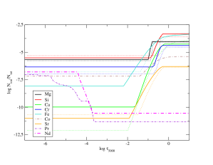
Figure 2: Stratification profiles of the final model with$T_{\rm eff}$= 7550 K and $\log g$= 3.8 (solid lines) and initial homogeneous model (dotted lines). Dash-dotted lines indicate elements that were not included in the initial model but added at a later stage.

Table 2: Stratification parameters for 7 elements based on the final model. Upper and lower atmospheric abundance values, abundance step position and width in column mass scale and deviation between observed and synthetic spectra are given. Formal errors of the DDAFit procedure are given.

	log$N/N_{\rm up}$	log$N/N_{\rm low}$	log$M_{\rm step}$	$\Delta$ log$M_{\rm step}$	dev
	$\pm$	$\pm$	$\pm$	$\pm$
Mg	-5.66	-4.03	0.06	0.04	2.8 %
	0.10	0.02	0.03	0.54
Si	-5.51	-3.33	0.17	0.16	1.7 %
	0.09	0.10	0.01	0.06
Ca	-9.98	-4.26	-0.02	0.56	3.2 %
	0.59	0.07	0.01	0.03
Cr	-6.30	-4.42	0.21	0.02	2.4 %
	0.06	0.10	0.01	0.10
Fe	-8.06	-3.16	-0.14	0.95	2.6 %
	0.78	0.28	0.04	0.19
Co	-7.16	-5.39	0.06	0.46	3.4 %
	0.16	0.41	0.05	0.36
Sr	-11.00	-6.30	-0.11	0.70	2.0 %
	0.73	0.22	0.04	0.17

Figure 3: Fit of observed (black) and synthetic lines with homogeneous (red) and stratified (blue) abundances. Fe is shown in the left column, Si in the right column.

4.1.1 Magnesium

Magnesium stratification profiles did not change significantly between the first and final iterations and were not sensitive to small atmospheric structure changes in any region. Analysis of the contribution functions indicates that the line set is sensitive to a variety of atmospheric depths, as it includes two rather strong Mg ii lines in the UV as well as a number of strong infrared lines, in addition to strong lines in the optical spectral region. The final stratification profile shows an abundance jump of 1.7 dex which is needed to reproduce observed line profiles.

4.1.2 Silicon

A variety of suitable Si lines were available for stratification analysis including five high excitation Si ii lines useful for probing deeper atmoshperic layers, two strong Si ii lines sensitive to upper atmospheric abundances, two infrared Si i lines as well as a number of Si i and Si ii lines that exhibit broad line wings. Throughout the iterative fitting process, the Si distribution remained stable between different iterations. The abundance jump of 2 dex is located in the same optical depth as for the Cr profile.

4.1.3 Calcium

Calcium shows the largest abundance stratification of all elements investigated in $10$ Aql with an abundance change of 5.7 dex between lower and upper atmospheric layers. The range of the transition region of the step profile was found to be $\log\tau_{\rm 5000}=[-0.2,-1.7]$. The upper atmospheric abundance was very sensitive to small changes in atmospheric structure occuring during the iterative model calculations, before reaching a converged solution. As many strong Ca lines with anomalously strong wings and shallow line cores were included in the analysis, the lower boundary of the abundance jump was constrained with better accuracy than the upper atmospheric abundance.

4.1.4 Chromium

Like Fe and Si, a variety of spectral lines was available for Cr analysis, including lines with high excitation energies, and strong UV lines which were found to be very sensitive to high atmospheric regions up to $\log\tau=-2$ according to the calculated contribution functions. The derived abundance profile remained very stable over all iterations and shows a small abundance gradient of 2 dex occuring in the same depth region as the Si abundance step.

4.1.5 Iron

Of all the investigated elements the highest number of suitable spectral lines for stratification calculations was found for Fe. Therefore the line list is expected to sample a large depth range of the stellar atmosphere. Two weak UV lines, two infrared lines, strong and weak lines of different ionization stages as well as high excitation Fe ii lines were included and a large final abundance gradient of 4.6 dex was derived. Inspection of the calculated contribution functions however revealed that only two strong lines were sensitive to higher atmospheric layers around $\log\tau=2$ while most other lines were mainly found to be formed between $\log\tau=-0.3$ and $-1.5$ in a stratified atmosphere. The upper atmospheric abundance was therefore very sensitive to small changes in atmospheric structure between different iteration steps. Nevertheless the lower atmospheric abundance, the position, and slope of the abundance gradient did not change significantly between first and final iterations.

4.1.6 Cobalt

The stratification analysis of Co became possible with the availability of better atomic line data, allowing to take into account hyperfine structure in spectrum synthesis. The coresponding data were taken from Pickering (1996) (Co i) and Bergemann et al. (2010) (Co ii). This is especially important as Co stratification is expected to be present (as indicated by the results of the abundance analysis) but not very strong. The final Co stratification was best represented by an abundance jump of 1.8 dex. This small abundance gradient (which was based on a short line list including strong UV lines and intermediate and weak optical lines) proved not to be very sensitive to small changes in model structure.

4.1.7 Strontium

Formation depth calculations predicted that the available set of Sr lines would be sensitive to a very narrow atmospheric region. Upper atmospheric abundance values were therefore found to be highly dependent on small changes in model structure and choice of input parameters for the fitting routine, throughout the iterative stratification fitting procedure. The final stratification profile of the converged model, however, did not differ significantly from the initial one. A large abundance gradient of 4.7 dex was fit to the observed line profiles by our algorithm. However, as the upper atmospheric abundance is constrained by only a few points in the line profiles of the strongest lines, the real size of the abundance jump might be overestimated.

4.1.8 Rare earth elements

For Pr and Nd we performed a NLTE stratification analysis as described in Mashonkina et al. (2005, 2009) using a trial-and-error method and the observed equivalent widths of the lines of the first and second ions, therefore the shape of the abundance profile may differ from a single-step function. Possible magnetic intensification for strong Nd iii lines was approximated by pseudomicroturbulent velocity of 1.0 km/s. The observed and calculated equivalent widths of Nd lines are illustrated in Fig. 4.

Pr and Nd are the only elements which are enriched in upper atmospheric layers between $\log\tau=-3.6$ and $-6.0$ and therefore required inclusion of inverted step profiles, compared to the other elements. The observed differences between upper and lower atmospheric abundances were 3.7 dex for Nd and 4.2 dex for Pr.

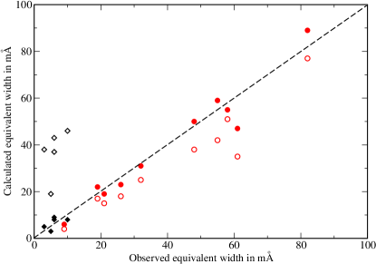
Figure 4: Comparison between the observed and calculated equivalent widths of Nd ii (diamonds) and Nd iii (circles) lines. Calculations are made with the derived Nd stratification in LTE (open symbols) and NLTE (filled symbols) approximations.

4.2 Fundamental and atmospheric parameters

Our determination of atmospheric parameters is based on the model fit to the observed energy distributions calibrated to absolute units (see Sect. 3.2.3). We note a discrepancy between space- and ground-based observations as can be seen from Fig. 5. In particular, data taken from the STIS archive are systematically lower than that of, e.g., broad-band spectrophotometry of Adelman et al. (1989) and Breger (1976) as well as fluxes computed from Johnson and Geneva photometric systems. In the attempt to fit these datasets one additional assumption about atmospheric chemistry was made. As follows from the computations of particle diffusion, helium always sinks in subphotosheric layers of A-F stars (Michaud et al., 1979). The same He depletion was found later also in the optically thin layers (Leblanc & Monin, 2004) suggesting that the atmospheres of CP stars of spectral types A-F may well be He-deficient. Having no spectroscopic clues about the true He stratification, we thus considered both He-normal (i.e. solar) and He-weak atmospheres with adopted He abundance of $\log(He/H)=-4$ (decreasing He abundance below this value has only marginal or no effect at all).

In addition, using observed spectral energy distributions and stellar parallaxes allowed us to derive the radius of the star. The latter is obtained by minimizing the deviation between observed and predicted fluxes for a given $T_{\rm eff}$ and $\log(g)$. The parallax $\pi=12.76\pm 0.29$ mas was taken from van Leeuwen (2007).

Making use of STIS data resulted in $T_{\rm eff}=7450$ K, $\log(g)=3.8$ both for He-normal and He-weak models. Formally, the He-weak model with $\log(g)=3.6$ provided a better fit with slightly lower $\chi^{2}$ compared to the model with $\log(g)=3.8$, but the computed mass of the star is then found to be $0.93M_{\odot}$ which is too small for an A-type star. Furthermore, the Paschen continuum, which is a good indicator of the atmospheric temperature, is clearly requiring a hotter temperature, which we find to be $T_{\rm eff}=7550$ K. The examples of the model predictions are shown on Fig. 5. The respective fundamental stellar parameters are: $R=2.53\pm 0.06R_{\odot}$, $M=1.47\pm 0.07M_{\odot}$, $L=17.78\pm 0.85L_{\odot}$ for $T_{\rm eff}=7450$ K model and $R=2.46\pm 0.06R_{\odot}$, $M=1.39\pm 0.07M_{\odot}$, $L=17.73\pm 0.88L_{\odot}$ for the $T_{\rm eff}=7550$ K model respectively. Note that the error-bars results from the parallax accuracy only.

As a next step we fitted the data obtained from ground-based observations. For this purpose we used spectrophotometric observations by Adelman et al. (1989) and extended them by NIR points ($\lambda>7000$Å) from Breger (1976). We did so because observations of Adelman cover the region of the Balmer jump and thus provide a homogeneous (in the sense of calibration) set of points in this important spectral region. In this particular case we find that He-normal models with $T_{\rm eff}=7450-7550$ K, $\log(g)=3.8$ and He-weak models with $T_{\rm eff}=7400-7450$ K, $\log(g)=3.8$ provide the best fit. The comparison of the observed and predicted fluxes is shown in Fig. 6. The respective fundamental stellar parameters for the He-normal and He-weak settings are given in table 3.

Table 3: Fundamental parameters for He-normal and He-weak models with $T_{\rm eff}$ corresponding to the best fits to observed fluxes.

	He-normal
$T_{\rm eff}$	7450 K	7550 K
R	$2.67\pm 0.06R_{\odot}$	$2.59\pm 0.06R_{\odot}$
M	$1.64\pm 0.08M_{\odot}$	$1.55\pm 0.07M_{\odot}$
L	$19.81\pm 0.90L_{\odot}$	$19.66\pm 0.90L_{\odot}$
	He-weak
$T_{\rm eff}$	7400 K	7450 K
R	$2.72\pm 0.06R_{\odot}$	$2.67\pm 0.06R_{\odot}$
M	$1.70\pm 0.08M_{\odot}$	$1.64\pm 0.08M_{\odot}$
L	$20.01\pm 0.90L_{\odot}$	$19.81\pm 0.90L_{\odot}$

Figure 7 illustrates a fit to the observed hydrogen Balmer line profiles for several models. It is seen that generally a model with $T_{\rm eff}=7450$ K provides an optimal fit to all three Balmer lines. On the other hand $\mathrm{H}\beta$ and $\mathrm{H}\gamma$ are best fitted with a slightly cooler $T_{\rm eff}=7400$ K He-weak model.

Taking into account a substantial scatter in the observed energy distributions, the derived atmospheric parameters of the star are $T_{\rm eff}=7500\pm 50$ K, $\log(g)=3.8\pm 0.1$. There are two major spectral regions that play a crucial role in the determination of atmospheric parameters: the Balmer jump (which controls best the value of surface gravity) and the Paschen continuum (which controls best the effective temperature). Therefore, it is important to use observed fluxes from the same data source that cover these two regions. Different calibration schemes applied by different observers could result in a systematic scatter in the derived model parameters. For instance, fluxes obtained by Breger lay slightly above the fluxes by Adelman in the region of the Balmer jump (see, e.g., top right panel of Fig. 5). Using them entirely in model fitting together with IUE data or UV points of Adelman results in a hotter best-fit temperature of $T_{\rm eff}=7550-7600$ K, compared to the one found by fitting data of Adelman extended with NIR points of Breger. Although this is not a large discrepancy, still one should be aware of similar systematics when analysing other stars for which no homogeneous datasets are available.

The difference between space- and ground-based observations results in radius uncertainity of $\Delta R=0.14R_{\odot}$ (assuming the same $T_{\rm eff}$ for reference models). This is a rather small discrepancy, which is of the same order as the errors provided by modern interferometry, as found by, e.g., Perraut et al. (2011) for another bright Ap star $\gamma$ Equ. Still, with improving interferometric accuracy, such a scatter between different observed spectrophotometric datasets could become important.

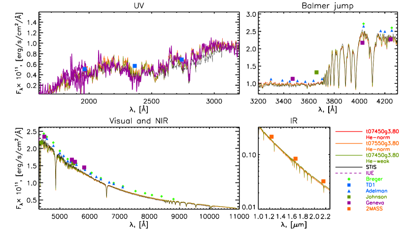
Figure 5: Comparison between observed and predicted fluxes of $10$ Aql. The model fit is done to the data obtained with STIS instrument. Please, see the online version of this figure for color-coding.

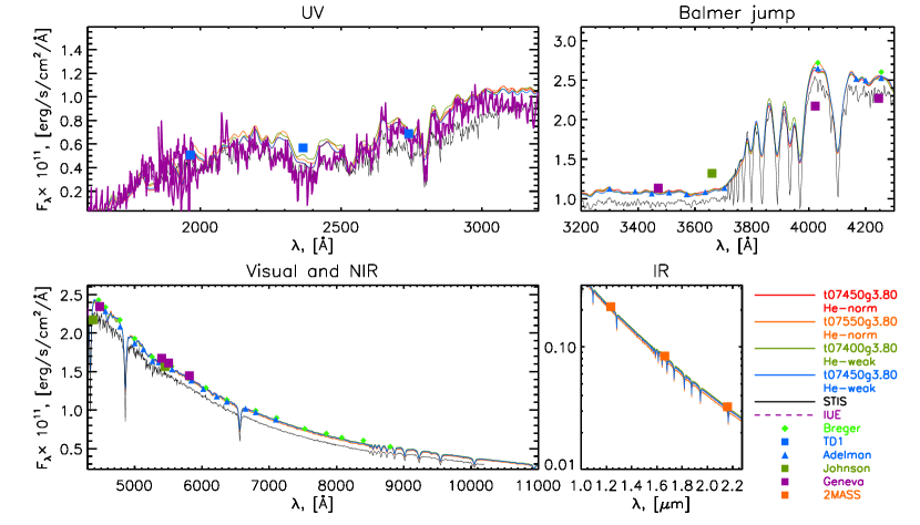
Figure 6: Same as on Fig. 5 but with the model fit to the ground-based spectrophotometric data of Adelman et al. (1989) and Breger (1976).

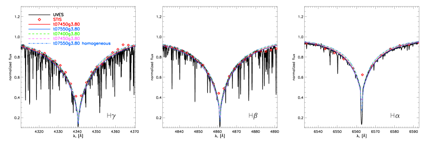
Figure 7: Observed Hydrogen Balmer lines compared to synthetic spectra calculated with different sets of fundamental parameters used during the iterative process. The dashed lines correspond to models computed with depleted He content.

To evaluate the influence of a change in model structure with modified He abundance on the derived stratification, two sets of profiles were computed using the He-weak and He-normal models with $T_{\rm eff}=7550$ K and $\log g=3.8$. Results of this comparison are shown in Fig. 8. A small systematic shift of abundance jumps towards lower atmospheric layers is observed when a He-weak composition is assumed. The quality of the fit of synthetic line profiles to observations was not found to be different between the two models.

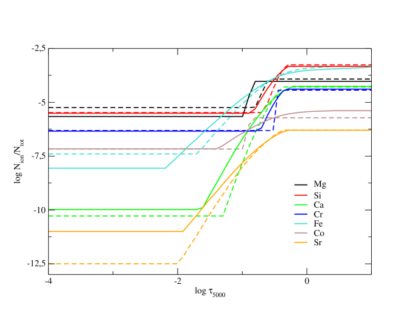
Figure 8: Comparison of stratification profiles of 7 elements computed with He-normal (solid lines) or He-weak (dashed lines) atmosphere models.

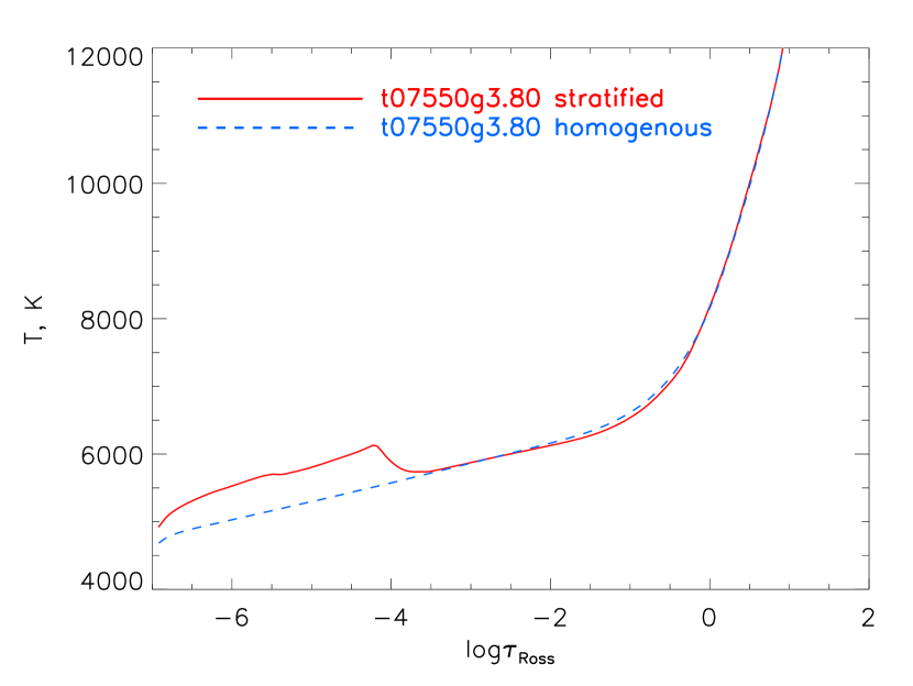
Figure 9: Temperature structure of models computed with homogeneous and stratified abundance patterns.

5 Discussion and conclusions

We have constructed a model atmosphere for $10$ Aql using a self-consistent iterative approach to derive atmospheric abundances and vertical chemical gradients by fitting models to the observed spectral lines and wide-range energy distributions.

By analyzing line profiles in a single spectrum we are able to derive somewhat mean vertical abundance gradients, i.e. gradients averaged over the visible surface of a star. It is to note that modern Doppler Imaging techniques (that rely on the rotationally modulated variability of line profiles) provide us with two-dimensional images of stellar surfaces and reveal non-uniform horizontal distributions of chemical elements and magnetic fields in atmospheres of CP stars. It is therefore natural to think of horizontal inhomogeneities as a result of variable vertical gradients, which depend on the local magnetic field geometry, hydrodynamic flows, and possibly other processes (that we don’t yet fully understand), the resulting force that pushes ions upwards or makes them diffuse downwards in the stellar atmosphere becomes variable over the stellar surface. That means that the positions of abundance jumps as well as their amplitudes are then the functions of local surface coordinates too. Only a self-consistent 3D mapping of stellar atmospheres has the potential of providing vertical and horizontal abundance gradients simultaneously from the same observed data sets. Modern theoretical models of atomic diffusion indeed predict a rather strong sensitivity of element stratification profiles to the geometry of the surface magnetic field (see, for example Leblanc et al., 2009; Alecian & Stift, 2010; Stift & Alecian, 2012).

However, the sharpness of spectral lines and lack of prominent line profile and magnetic field variations imply a very long rotational period for 10 Aql (Ryabchikova et al., 2005; Sachkov et al., 2008). In this situation we are not able to use Doppler imaging to constrain surface distributions of chemical elements. Very weak long-term line profile variability detected by (Sachkov et al., 2008) suggests that horizontal abundance gradients in this star are not large or that the star is viewed from nearly the same aspect angle during its rotation cycle. We have estimated that this weak variability would result in a mean abundance difference of $\leq$0.05 dex. Therefore, we do not expect stratification analysis to be significantly affected by horizontal inhomogeneities.

Our approach of using step-like assumption on derived abundance gradients has obvious limitations. First of all it is limited to a very narrow atmospheric region where a given set of atomic lines used in stratification analysis is formed. It naturally cannot predict abundances in optically very thin and thick layers which we simply do not see with our instruments. Secondly, it is impossible to restore any kind of complex vertical distribution whose shape may strongly deviate from a step-like assumption (see, for example Leblanc et al., 2009; Alecian & Stift, 2010; Stift & Alecian, 2012). However, what is important for us is to see a general trend of element distributions as a function of depths, i.e. whether a given element is being brought upwards or downwards in the line forming region of a stellar atmosphere and how strong the resulting abundance gradient is. In spite of its limitations this approach is suitable of tracking any kind of systematic as applied to different stars with, e.g., different temperatures and surface magnetic fields.

The detailed analysis of the high resolution spectra ranging from UV to infrared regions indicated that robustness of the inferred vertical stratification profiles is very much dependent on the sensitivity of the selected line set to a wide range of atmospheric depths. As seen, e.g. in our analysis of Cr stratification, inclusion of high- and low-excitation lines helps to constrain parameters describing a chemical gradient best. However, upper atmospheric abundances are sometimes still only constrained by a few lines which are sensitive to high atmospheric layers. Therefore the value of the upper atmospheric abundance might vary between an initial homogeneous model atmosphere and a stratified model found after the iterative calculations have converged.

The mean abundances for non-stratified elements changed by about 0.1 dex between the homogogeneous starting model and all other stratified models. Abundance variations between different stratified models were negligible.

The most striking change between our homogeneous starting model and the final stratified model atmosphere is seen in a systematic shift of the abundance jumps towards higher atmospheric layers in the stratified case.

Between the first and final models, derived stratification profiles were used to calculate synthetic flux distributions to be compared with a large number of observations. This comparison was used for fine tuning of fundamental parameters of $10$ Aql. We find that stratification itself has little effect on the synthetic energy distribution of the star compared to models computed with individual and homogeneous abundances. The overall fit and derived radii were almost identical. Therefore individual abundances appear to be the most important ingredient in the SED modelling, at least in the roAp temperature region. On the other hand, we do find that the observed hydrogen lines could not be reproduced with chemically homogeneous model atmospheres, as illustrated on Fig. 7 where we also show two He-normal models with $T_{\rm eff}=7550$ K, $\log(g)=3.8$ computed with stratified and homogeneous abundances. Therefore, the inclusion of vertical element stratification has to be preferred when trying to establish an atmosphere model for a single Ap star in order to reproduce spectroscopic and SED observation simultaneously.

Similar to the case of HD 24712 (Shulyak et al., 2009) we find a strong influence of REE opacity in the surface atmospheric structure of stratified models. In particular, strong abundance gradients of Pr and Nd shown in Fig. 2 lead to a heating of plasma and appearance of the characteristic temperature jump. This is illustrated on Fig. 9 for He-normal final models. Interesting to note that such a temperature jump was first empirically predicted by Kochukhov et al. (2002) in order to fit narrow region of Balmer line profiles between wings and core (the so-called core-wing anomaly). Unfortunately, the temperature jump predicted by our models is located way too high in the atmosphere compared to what was suggested by Kochukhov et al. (2002) (see their Fig. 3). We hope that a self consistent NLTE modelling of REE stratification will help to improve existing models and finally match the predicted position of the temperature jump. Last but not least, the incorporation of an atmospheric model with an inverse temperature gradient from Shulyak et al. (2009) allowed to improve pulsation models of HD 24712 as recently computed by Saio et al. (2010). All this suggests that the temperature structure of Ap stars is indeed very much different from the “canonical” $T-\tau$ relation and that the derived temperature jumps are real.

One of the important results of the present study is the decrease of the $\log(g)$ value from $4.0$ to $3.8$ once the fitting of SED is introduced in the atmospheric analysis. This is caused by the incorporation of realistic chemistry in model atmosphere computations as well as the use of homogeneous spectral energy distributions (i.e. STIS data in this particular case) which cover the whole Balmer jump region. A similar decrease of surface gravity was also required in two previous investigations of Ap stars $\alpha$ Cir (Kochukhov et al., 2009) and HD 24712 (Shulyak et al., 2009). In the latter case, recent pulsation modelling by Saio et al. (2010) also suggested that $\log(g)$ of HD 24712 should be lower than what we usually find from photometric calibrations of Ap stars. From our analysis we conclude that a decrease of $\log(g)$ is consistent with all observations if the appropriate abundance pattern is included in model calculations. On the other hand, decreasing surface gravity does not dramatically change stratification profiles (see our first and final profiles in Fig. 2).

One of the open questions that still needs to be answered is the true helium content in the atmospheres of Ap stars. Using available observational material it is impossible to distinguish between He-normal and He-weak models with high accuracy. Surface temperatures of roAp stars are too low to see He lines. The helium concentration formally influences the quality of the fit to energy distributions, but once plotted against low and moderate resolution data the difference is difficult to see, except for the Balmer jump region. In addition, hydrogen line profiles are also only marginally affected by He depletion. Pulsation calculations may therefore assume He depletion and still be compatible with all available observations (spectroscopy, spectrophotometry). Again, improved self-consistent diffusion models are probably the right way to go, in the search for a definite answer.

Table 4: Atomic parameters for all lines used in stratification analysis of 10 Aql. Abbreviations of references correspond to different internal line lists of VALD and individual line lists with observed parameters. In case broadening constants were absent in VALD, approximations were used.

Ion	$\lambda$ [Å]	$\log gf$	$E_{\rm low}$	$\gamma_{\rm Stark}$	Ref.
Mg i	4702.99	-0.420	4.346	-4.460	Bu
Mg i	4730.02	-2.409	4.346	approx	JK
Mg i	5172.68	-0.380	2.712	-5.470	Wi
Mg i	5183.60	-0.160	2.717	-5.470	Wi
Mg i	5528.40	-0.400	4.346	-4.460	Bu
Mg i	5711.08	-1.833	4.346	approx	Ku
Mg i	8806.75	-0.200	4.346	approx	$\odot$
Mg i	8923.56	-1.650	5.394	approx	LL
Mg ii	3104.71	-0.030	8.864	-3.970	Ku
Mg ii	3104.72	-1.330	8.864	-3.970	Ku
Mg ii	3104.80	-0.190	8.864	-3.970	Ku
Mg ii	4390.51	-1.700	9.999	-4.070	Wi
Mg ii	4390.57	-0.530	9.999	-4.070	Wi
Mg ii	4427.99	-1.200	9.996	-4.400	Wi
Mg ii	4433.98	-0.900	9.999	-4.400	Wi
Mg ii	4481.12	0.740	8.864	-4.700	Ku
Mg ii	4481.15	-0.560	8.864	-4.700	Ku
Mg ii	4481.32	0.590	8.864	-4.700	Ku
Mg ii	7877.05	0.390	9.996	-4.540	Wi
Mg ii	8213.98	-0.950	9.999	-4.770	$\odot$
Si i	5517.55	-2.384	5.080	8.380	BR
Si i	5645.03	-2.400	5.614	approx	NL
Si i	5665.56	-2.040	4.920	8.290	LL
Si i	5684.49	-1.650	4.950	8.250	NL
Si i	5690.43	-1.870	4.930	8.300	NL
Si i	5701.10	-2.050	4.930	8.310	NL
Si i	6125.02	-1.513	5.610	approx	sH
Si i	6131.57	-1.705	5.610	approx	sH
Si i	6131.85	-1.685	5.610	approx	sH
Si i	6142.48	-1.420	5.620	approx	BR
Si i	6155.13	-0.770	5.619	approx	BR
Si i	6244.47	-1.363	5.610	approx	sH
Si i	7017.66	-1.070	5.870	approx	sH
Si i	7034.90	-0.780	5.871	8.140	BR
Si ii	5055.98	0.440	10.074	9.040	AJPP
Si ii	5056.31	-0.359	10.074	9.030	NL
Si ii	5632.96	-0.820	14.186	approx	Wil
Si ii	5688.81	0.000	14.186	approx	Wil
Si ii	5957.55	-0.350	10.067	8.820	AJPP
Si ii	6347.10	0.290	8.121	9.090	Wil
Si ii	6371.37	-0.080	8.121	9.080	NIST
Si ii	6660.53	0.230	14.504	approx	Wil
Ca i	4226.72	0.244	0.000	-6.030	SG
Ca i	5857.45	0.240	2.933	-5.420	S
Ca i	5867.56	-1.570	2.933	-4.705	S
Ca i	6162.17	-0.090	1.899	-5.320	SN
Ca i	6163.75	-1.286	2.521	-4.998	SR
Ca i	6169.04	-0.797	2.523	-4.997	SR
Ca i	6169.56	-0.478	2.526	-4.994	SR
Ca i	6455.59	-1.340	2.523	-6.072	S
Ca i	6471.66	-0.686	2.526	-6.072	SR
Ca ii	5021.13	-1.207	7.515	-4.612	TB
Ca ii	6456.87	0.410	8.438	-3.711	TB
Ca ii	8248.79	0.556	7.515	-4.600	TB
Cr i	3355.73	-1.107	3.847	-5.118	GF
Cr i	5065.91	-1.340	2.708	-6.209	GF
Cr i	5110.74	-1.289	2.709	-6.210	GF
Cr i	5204.50	-0.208	0.941	-6.154	MFW
Cr i	5247.56	-1.640	0.961	-6.120	MFW
Cr i	5296.69	-1.400	0.983	-6.120	MFW
Cr i	5345.80	-0.980	1.004	-6.117	MFW
Cr i	5368.53	-1.033	3.847	-6.104	GF
Cr i	6762.41	-0.555	5.280	-5.246	GF
Cr i	6762.42	-0.092	5.282	-5.259	GF
Cr ii	3308.13	-1.094	4.920	-6.627	RU
Cr ii	3311.93	-0.510	4.156	-6.648	RU
Cr ii	3338.80	0.053	6.792	-5.671	RU
Cr ii	3355.65	-0.809	6.747	-5.670	RU
Cr ii	3378.33	-1.045	3.104	-6.716	RU
Cr ii	5024.52	-1.733	6.285	-6.652	RU
Cr ii	5085.65	-2.215	5.871	-6.643	RU
Cr ii	5210.82	-3.259	4.042	-6.720	RU
Cr ii	5210.86	-2.941	3.758	-6.584	RU
Cr ii	5232.49	-2.360	4.071	-6.639	RU
Cr ii	5379.79	-2.081	7.331	-6.558	RU
Cr ii	5678.39	-1.496	6.484	-6.627	RU
Cr ii	6418.90	-1.915	6.686	-6.603	RU
Fe i	3354.05	-1.169	2.858	-6.091	V2
Fe i	3356.68	-1.554	3.047	-5.082	GF
Fe i	4404.75	-0.142	1.557	-6.204	V2
Fe i	5198.71	-2.135	2.223	-6.185	V2
Fe i	5324.17	-0.103	3.211	-5.496	V2
Fe i	5367.46	0.443	4.415	-5.133	V2
Fe i	5410.90	0.398	4.473	-5.060	V2
Fe i	5434.52	-2.122	1.011	-6.303	V2
Fe i	5436.29	-1.540	4.386	-4.997	V2
Fe i	5445.04	-0.020	4.386	-4.582	V2
Fe i	5546.50	-1.310	4.371	-6.109	V2
Fe i	5560.21	-1.190	4.434	-4.323	V2
Fe i	5576.08	-1.000	3.430	-5.491	V2
Fe i	5862.35	-0.058	4.549	-4.582	GF
Fe i	6136.61	-1.400	2.453	-6.327	V2
Fe i	6137.69	-1.403	2.588	-6.112	V2
Fe i	6165.36	-1.474	4.143	-6.156	V2
Fe i	6173.33	-2.880	2.223	-6.194	V2
Fe i	6219.28	-2.433	2.198	-6.202	V2
Fe i	6421.35	-2.027	2.279	-6.310	V2
Fe ii	4923.92	-1.504	2.891	-6.583	RU
Fe ii	5015.75	-0.028	10.348	-5.287	RU
Fe ii	5045.11	-0.002	10.308	-4.984	RU
Fe ii	5047.64	-0.235	10.308	-4.976	RU
Fe ii	5061.71	0.284	10.308	-5.189	RU
Fe ii	5197.57	-2.348	3.230	-6.599	RU
Fe ii	5291.66	0.544	10.480	-5.468	RU
Fe ii	5325.55	-3.324	3.221	-6.603	RU
Fe ii	5362.86	-2.616	3.199	-6.666	RU
Fe ii	5534.84	-2.865	3.245	-6.601	RU
Fe ii	6432.68	-3.687	2.891	-6.687	RU
Fe ii	6516.08	-3.432	2.891	-6.686	RU
Fe ii	7449.33	-3.488	3.889	-6.668	RU
Fe ii	7711.72	-2.683	3.903	-6.666	RU
Co i	3502.27	0.070	0.432	-6.300	FMW
Co i	3502.61	-1.240	0.174	-6.374	FMW
Co i	4813.46	0.050	3.216	-5.627	GF
Co i	5342.69	0.690	4.021	-4.928	GF
Co i	5347.49	-0.160	4.149	-4.952	GF
Co i	6082.42	-0.520	3.514	-5.474	GF
Co ii	3415.77	-1.740	2.203	-6.675	SLW
Co ii	3501.71	-0.970	2.203	-6.673	T83av
Sr i	4607.32	-0.570	0.000	approx	Bh
Sr i	4722.27	-0.220	1.798	approx	GC
Sr i	4741.91	-0.410	1.775	approx	GC
Sr i	4784.31	-0.510	1.798	approx	Bh
Sr i	4811.87	0.190	1.847	approx	GC
Sr i	5222.19	-0.380	2.251	approx	GC
Sr i	5229.26	-0.330	2.259	approx	GC
Sr i	5450.83	-0.340	2.259	approx	GC
Sr i	5486.13	-0.460	2.251	approx	GC
Sr i	5504.17	0.090	2.259	approx	GC
Sr i	5521.76	-0.060	2.251	approx	GC
Sr i	5540.04	-0.410	2.259	approx	GC
Sr i	6408.45	0.510	2.271	approx	GC
Sr i	6503.99	0.320	2.259	approx	GC
Sr i	7070.07	-0.030	1.847	approx	GC
Sr ii	3380.70	0.199	2.940	approx	Bh
Sr ii	3464.45	0.487	3.040	approx	Bh
Sr ii	7334.95	-1.102	7.562	approx	Bh
Nd ii	5130.59	0.45	1.304	-5.61	HLSC
Nd ii	5165.13	-0.74	0.680	approx	HLSC
Nd ii	5255.51	-0.67	0.205	approx	HLSC
Nd ii	5293.16	0.10	0.823	-5.74	HLSC
Nd ii	5319.82	-0.14	0.550	-5.82	HLSC
Nd iii	5102.16	-0.62	0.296	approx	RRKB
Nd iii	5294.11	-0.69	0.000	approx	RRKB
Nd iii	5677.18	-1.45	0.631	approx	RRKB
Nd iii	5802.53	-1.71	0.296	approx	RRKB
Nd iii	5845.02	-1.18	0.631	approx	RRKB
Nd iii	5851.54	-1.55	0.460	approx	RRKB
Nd iii	6145.07	-1.33	0.296	approx	RRKB
Nd iii	6327.26	-1.41	0.141	approx	RRKB
Nd iii	6550.23	-1.49	0.000	approx	RRKB
Nd iii	6690.83	-2.46	0.460	approx	RRKB
Pr ii	4222.90	0.271	0.055	approx	ILW
Pr ii	5322.77	-0.319	0.483	approx	ILW
Pr iii	5299.99	-0.720	0.359	approx	ISAN
Pr iii	6090.01	-0.871	0.359	approx	ISAN
Pr iii	6160.23	-1.020	0.173	approx	ISAN
Pr iii	6195.62	-1.071	0.000	approx	ISAN
Pr iii	7030.39	-0.929	0.359	approx	ISAN
Pr iii	7781.98	-1.276	0.000	approx	ISAN

Table 4: continued.

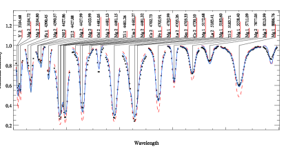
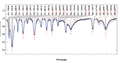
Figure 10: Fit of observed (black) and synthetic lines with homogeneous (red) and stratified (blue) abundances. Mg is shown in the left column, Ca in the right column.

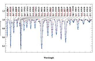
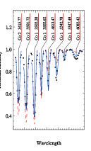
Figure 11: Fit of observed (black) and synthetic lines with homogeneous (red) and stratified (blue) abundances. Cr is shown in the left column, Co in the right column.

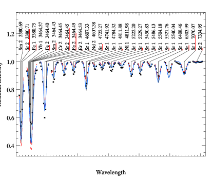
Figure 12: Fit of observed (black) and synthetic Sr lines with homogeneous (red) and stratified (blue) abundances.