Duality for stochastic models of transport
Abstract
We study three classes of continuous time Markov processes (inclusion process, exclusion process, independent walkers) and a family of interacting diffusions (Brownian energy process). For each model we define a boundary driven process which is obtained by placing the system in contact with proper reservoirs, working at different particle densities or different temperatures. We show that all the models are exactly solvable by duality, using a dual process with absorbing boundaries. The solution does also apply to the so-called thermalization limit in which particles or energy is instantaneously redistributed among sites.
The results shows that duality is a versatile tool for analyzing stochastic models of transport, while the analysis in the literature has been so far limited to particular instances. Long-range correlations naturally emerge as a result of the interaction of dual particles at the microscopic level and the explicit computations of covariances match, in the scaling limit, the predictions of the macroscopic fluctuation theory.
1 Introduction
Interacting particle systems are classical models to study non-equilibrium statistical mechanics. The standard setting is the one in which a system is placed in contact with reservoirs working at different parameters that create a stationary state characterized by a non-zero averaged current. The prototypical example are the Symmetric Exclusion process with at most one particle per site connected to birth and death process at the boundaries [L, D] and the KMP process [KMP] connected to reservoirs which impose at the boundaries Boltzmann-Gibbs distribution with different temperatures. The Symmetric exclusion process is a model for transport of a discrete quantity, whereas the KMP process models transport of a continuous quantity.
Problems that are very hard for classical Hamiltonian systems – for instance deriving Fourier law starting from the microscopic evolution – can be successfully approached using stochastic models. Furthermore stochastic models of transport have been used to prove new theorems in non-equilibrium statistical mechanics, such as the fluctuation theorem [GC, K], to introduce new principles, such as the additivity principle [BD], to construct new schemes, such as the macroscopic fluctuation theory that describes the density and current large deviations for diffusive systems [BDGJL1, DLS], to test new algorithms, such as cloning algorithms to simulate rare events [GKLT]. Recently, the connection between deterministic Hamiltonian systems and stochastic models is emerging either by considering evolutions in which they are coupled [BO] or by considering slow/fast variables [DL] and thermodynamic formalismo [LAW].
An important tool in the study of interacting stochastic systems is duality [S, L]. Duality provides the connection between a process and a simpler dual process. This technique has been applied in different contexts, including interacting particles systems, interacting diffusions, queueing theory and mathematical population genetics. For a recent review on duality, which also include many references, see [JK]. For recent applications of duality in the context of asymmetric processes and KPZ universality see [BCS].
In the context of interacting particle systems or interacting diffusion processes modeling non-equilibrium systems, the main simplification coming from duality lies in the fact that for an appropriate choice of the modeling of the boundary reservoirs, a dual process exists where the reservoirs are replaced by absorbing boundaries. This was originally found for the boundary driven Symmetric Exclusion process with at most one particle per site [Spo] and for the KMP model [KMP]. As a consequence, the -point correlation functions in the non-equilibrium steady state can be obtained from absorption probabilities of dual particles. In particular, the stationary density or temperature profile can be easily obtained from a single dual walker. Other simplifications due to duality include “from continuous to discrete”, i.e., connecting continuous systems with discrete particle systems and “from many to few”, i.e., correlation functions in a systems of possibly infinitely many particles reduce to as many dual particles as the degree of the correlation function.
In this paper we introduce and study a large class of boundary driven processes which can be dealt with via this technique of duality. We treat processes with interactions of “inclusion” (attractive) and “exclusion” (repulsive) type.
The particle systems range from the Symmetric Inclusion Processes (SIP) with Negative-Binomial product stationary measures at equilibrium, to the Symmetric Exclusion Processes (SEP) having a Binomial product measures as equilibrium state, via Independent Random Walkers (IRW) with a product Poisson stationary measures. The interacting diffusions corresponding to the SIP are given by the so-called Brownian Energy processes (BEP), having product of Gamma distributions as equilibrium.
We also study “thermalized versions” of these processes. For the diffusion models thermalization leads to “energy redistribution models” of which the famous KMP model is a particular instance. For particle systems thermalization leads to “occupation redistribution models” where in one event associated to a nearest neighbour edge, occupations of particles are reshuffled according to a specific redistribution measure. The dual KMP model is a particular instance of these thermalized particle systems. Most of these thermalized models are new, as well as their boundary driven versions. A non-trivial stationary state is found for these boundary driven thermalized models even considering only one site, since the reservoirs are not additive.
Some of the processes we discuss here have already been introduced before: we have chosen to include all of them, including independent random walkers, in order to provide a (up to know and to our knowledge) complete and self-contained overview of the interacting non-equilibrium systems that can be treated with duality. The main message of this paper is thus an extension of duality and its consequences into the boundary driven non-equilibrium setting for all the models discovered and studied in [GKR, GKRV, GRV].
2 Models definition
In this section we introduce
our models.
In the most complete setting,
they are constituted by a bulk which is kept in a non equilibrium state
by the contact with particles or energy reservoirs.
In particular, we consider one-dimensional systems
on a finite lattice , whose boundaries
(i.e. sites and )
interact with the reservoirs. When needed, the reservoirs themselves will be represented by two extra sites, namely sites and .
Accordingly, the generators of the random processes associated with our models can be generically expressed as the sum of three terms
| (2.1) |
where represents the generator of the dynamics in the bulk, while and represent the generators of the reservoirs.
We will consider four models: three classes of interacting particle systems, characterized by the different interactions between the particles, and one family of interacting diffusions introduced to model heat conduction
[GKR, GKRV, GRV]. The models are:
-
1.
the Symmetric Inclusion Process (SIP), with attractive interaction between neighbouring particles;
-
2.
the Symmetric Exclusion Process (SEP), with repulsive interaction between neighbouring particles;
-
3.
the Independent Random Walkers (IRW), without interactions among particles;
-
4.
the Brownian Energy Process (BEP).
In the first three cases the dynamic variable is a vector that specifies the number of particle on each site: ; here , the state space, depends on the model and will be defined ahead. In the case of the BEP the dynamic variable is a vector representing the energies on each site of the lattice: .
2.1 Interacting particle systems
The generators of the reservoirs for SIP, SEP and IRW have the following general form:
| (2.2) | |||||
| (2.3) |
Here
denotes the configuration obtained
from by moving a particle from site to site ,
i.e. .
According to (2.2) and (2.3) particles are injected into the system through the boundaries
with rate with , and removed from the same sites with rate . While is
model-dependent, the annihilation rate is not, being in any case proportional to the number of
particles at the boundary site.
We introduce now our models by defining the actions of the generators on the functions .
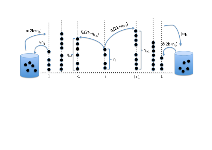
Inclusion walkers SIP(). The inclusion process (without boundaries) is introduced first in [GKR], and also studied further in [GRV].
In the SIP(), see Figure 1, each site can accomodate an arbitrary number of particles, thus . In the bulk each particle may jump to its left or right neighbouring site with rates proportional to the number of particles in the departure site and to the number of particles in the arrival site. In each boundary site particles are created with a rate proportional to plus the number of particles sitting in that site; labels the class of models. The generator is
The positive numbers and (resp. and ) tune the creation and annihilation rates of the left (resp. right) reservoirs.
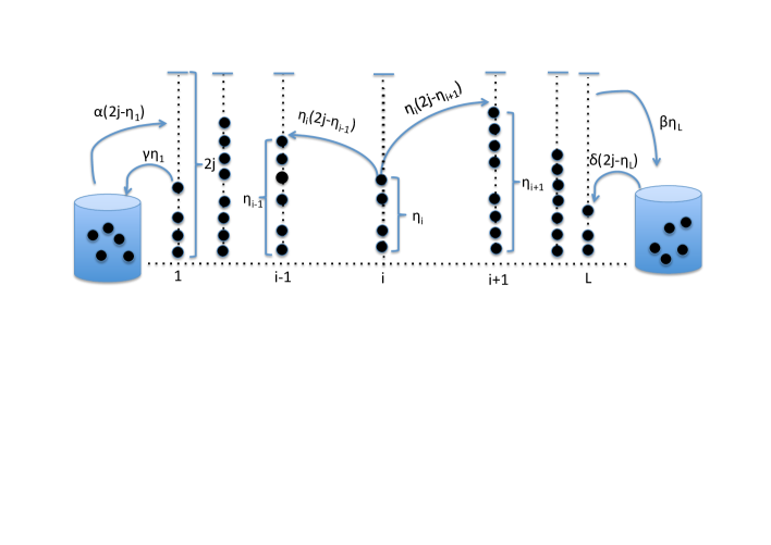
Exclusion walkers SEP(). For the boundary driven simple exclusion process has been studied using duality in [Spo]. The model for arbitrary has been introduced and studied in [SS]. From the mathematical point of view a related model which also exhibits product measures, but which does not have the self-duality property is studied (without boundary reservoirs) in [Keis].
In the SEP() the maximum occupation number at each site is , thus . In the bulk particles jump independently to nearest neighbouring lattices sites at rate proportional to the number of particles in the departure site times the number of holes in the arrival site. The reservoirs inject particles in the systems with a rate proportional to the holes in the boundary sites, see Figure 2. The generator is
The parameters have the same meaning as in the SIP().
Independent random walkers IRW. This well-known model is first considered in [S], and with boundaries is also well-known and studied e.g. in [LMS] (where also the more general boundary driven zero range process is studied).
In the IRW model each particle jumps independently to nearest neighbouring lattices sites at rate 1, and each site can accomodate an arbitrary number of particles, thus . Jumps occur with the same probability to the right and to the left, while particles are created at rates and irrespective of the numer of particles at the boundaries. Therefore the system is described by the generator
The dynamics in the bulk can be further described by saying that if at site there are particles, one of the particle jumps at rate either to the left or to the right. As in the previous cases, parameters and define the annihilation processes.
Remark 2.1.
The effect of the reservoirs is to impose the average number of particles
on the left and on the right sides of the chains.
With some misuse of language, but sticking to standard notations, we will call “densities” these averages and we will denote them (left reservoir)
and (right reservoir). The vaules of and are reported in the table below and computed in Sec.3.
System SIP SEP IRW
Remark 2.2.
Note that the SIP process requires and . This condition turns out to be necessary in order for the system to reach a stationary state (see also formula (3.8)).
Remark 2.3.
It is interesting to remark that the exclusion (resp. inclusion) walkers with parameters converges to the independent walkers with parameters in the limit (resp. ) under the scaling , (resp. , ). Indeed, in this limit the generators and converge to . This remark can be put on rigorous grounds by using the Trotter-Kunz theorem (see Theorem 2.12 of [L]); see for istance [GKRV] for the proof in the case of SEP().
2.2 Interacting diffusions
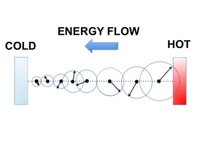
The last process we consider is the Brownian Energy Process (BEP), originally introduced (without boundaries) in [GKRV]. Here we present its boundary driven version. The bulk diffusion process of the BEP also appears in genetics, as the multi-type Wright-Fisher diffusion with parent independent mutation rate (see [CGGR] and references therein for a discussion of duality in the context of population dynamics).
Brownian energy process BEP(). This model describes symmetric energy exchange between nearest neighbouring sites, see Figure 3. The dynamical variables (energies) are collected in the vector and the generator is
Remark 2.4.
The origin of the bulk dynamics, generated by
| (2.8) |
can be explained as follows [GKR, GKRV]. Consider velocity variables on each site and call them with . Suppose that they evolve with the following generator
| (2.9) |
which defines a process, called Brownian Momentum Process, introduced in [BO, GK]. Each term in represents a rotation in the plane , therefore it conserves the total length , i.e. the total kinetic energy. One can check that the BEP is the evolution process, induced by (2.9), of the total energies on each site
| (2.10) |
The generator of the BEP reservoirs and , that will be discussed in some details in Sec. 3, impose an average energy on the left, and an average energy on the right. The choice of their form is motivated as follows. Consider an Ornstein-Uhlenbeck process on each of the velocities at site of the Brownian Momentum process (2.9), namely
| (2.11) |
Since in the stationary state of this reservoir the are independent centered Gaussian with variance then, using (2.10), the expectation of is .
2.3 Scaling limit of the particle systems
Besides duality, there is another relation connecting the bulk part of the BEP with generator (2.8), and the bulk part of the SIP with generator (third line in (2.1)). The BEP can be indeed obtained from the SIP, through a suitable scaling limit, by a reinterpretation of this process as a model of energy transport, by supposing that each particle carries a quantum of energy . In this interpretation, since conserves the number of particles, then it conserves the total energy. Consider the free boundary inclusion process generated by and let be the total number of particles, i.e. . Let be a parameter of the order of , then one expects to be of the order of as (despite attractive interactions for any finite there are no condensation phenomena in the SIP; one needs to rescale with to see particles coalescing into a single site; see [GRV2]). Then one may investigate the continuous dynamics generated in the limit as on the variables . It turns out that the limiting dynamics for is generated by .
Proposition 2.5.
Let be the bulk inclusion process generated by with particles. Let for some fixed . Then the process where is, in the limit , the bulk Brownian energy process generated by with total energy .
Proof. Let , be a two times countinuously differentiable function, i.e. . Let be such that , then for any as above, there exists , , such that
| (2.12) |
Let be the generator of the process induced by the SIP, then acts on as follows:
Suppose that converges to a finite limit as . Then, from the regularity assumptions on , we have
| (2.13) | |||||
while
| (2.14) | |||||
and
Therefore we have
| (2.15) |
Thus, for any as above, . Moreover the total energy is clearly conserved in the limit and it is given by . ∎
The same scaling analysis of the inclusion walkers can be performed on the bulk dynamics of independent random walkers. This yields a deterministic process as scaling limit, which is also dual to independent random walkers (cfr. [GKRV]).
Proposition 2.6.
Let be the bulk process generated by with particles. Let for some fixed . Then the process where is, in the limit , the deterministic energy process (DEP) with total energy generated by
Remark 2.7.
One may wonder whether there exists a diffusion process arising as a limit of the Exclusion process. By performing an analogous scaling as above, the rates of the SEP take the form that become negative in the limit as . Consistently the limit of the SEP generator is a second order differential operator that cannot be interpreted as the generator of a Markov process, since it is has a negative coefficient in front of the second order derivatives, i.e.
| (2.16) |
Remark 2.8.
The same scaling limit which transfoms the bulk dynamics of the SIP into the one of the BEP does not work with the reservoirs. Indeed, applying to the scaling of Propositon 2.5, the resulting generator is
| (2.17) |
which produces a deterministic behavior: . On the other hand it is simple to check that the thermal bath of the BEP can be obtained from a boundary driven SIP with a modified reservoir generated by
| (2.18) |
with the condition as .
3 Stationary measures at equilibrium
The models introduced in the previous section are Markov processes with discrete or
continuous state spaces. The long term behaviour of the processes are described by their stationary measures.
In general it is hard to determine such measures and, in fact, the invariant states of SIP, SEP and BEP
in non-equilibrium conditions are not explicitly known.
The problem of finding the explicit form of the invariant states is greatly
simplyfied at equilibrium. The equilibrium condition for our systems can be obtained in two ways: either by suppressing the reservoirs
(i.e. considering only the bulk dynamics ) or, retaining the reservoirs, by imposing equal densities
or equal temperatures at the boundaries of the chain, i.e. or .
In the first case there exists an infinite family of reversible measures labelled by a continuous parameter.
In the second case (i.e. in the presence of the reservoir) at density (resp. at temperature ) the boundary conditions select one reversible measure.
3.1 Equilibrium product measures
Reversible invariant probability measure of the bulk dynamics generated by can be obtained by imposing the detailed balance condition. When the state space is finite or countable, this condition is expressed by requiring that for any pair of configurations the probability satisfies
| (3.1) |
where is the transition rate from the configuration to , i.e. with . When the state space is continuos, a probability measure with density is said to be reversible stationary measure if, for all functions and in the domain of the generator , it holds
| (3.2) |
By imposing (3.1) in the case of SIP, SEP, IRW and (3.2) in the case of BEP and requiring the factorization of the probability measure one obtain the reversible measures described in the following proposition, whose proof is left to the reader.
Proposition 3.1.
For the bulk processes with generator defined in Sec. 2 we have
Inclusion walkers SIP()
The process with generator has a reversible stationary measure
given by products of generalized Negative Binomial measures with parameters
and arbitrary , i.e.
| (3.3) |
Exclusion walkers SEP()
The process with generator has reversible stationary measure
given by products of Binomial measures with parameters and arbitrary , i.e.
| (3.4) |
Independent random walkers IRW
The process with generator has reversible stationary measure
given by products of Poisson distribution with
arbitrary parameter i.e.
| (3.5) |
Brownian energy process BEP()
The process with generator has reversible measures given
by product of Gamma distributions with
parameters and arbitrary , i.e.
| (3.6) |
3.2 Equilibrium product measure with reservoirs
We recall that, in the case of particle systems (see Sec.2),
the reservoirs are modeled by birth-death processes with creation rate and annihilation rate , the number of particles at the boundary. Each reservoir has, thus, its own
reversible invariant probability measure, , which satisfies the detailed balance condition . This condition can be used to compute . The average value of the random number (that we call density, irrespective to its value) is the quantity imposed by the reservoir to the system.
The effects of the reservoirs, under the equilibrium conditions, are described in the following proposition, which can easily be proved with an explicit computation.
Proposition 3.2.
For the processes with generator defined in Sec. 2 we have:
Inclusion walkers SIP()
The left reservoir is modeled by the birth and death process with
rates
| (3.7) |
The stationary state of this reservoir is given by a Negative Binomial measure with parameters and . The reservoir density is . The boundary driven process with generator defined in (2.1), with parameters and such that (and thus ) admits the stationary product distribution:
| (3.8) |
Exclusion walkers SEP ()
The left reservoir is modeled by
| (3.9) |
The stationary state of this reservoir is given by a Binomial measure with parameters and . The reservoir density is . The boundary driven process with generator defined in (2.1), with parameters and such that (and thus ) admits the stationary product distribution:
| (3.10) |
Independent random walkers IRW
The left reservoir has a constant birth rate
| (3.11) |
This reservoir imposes a Poisson measure with parameter . Therefore the density (i.e. mean number of particle) is . If the process with generator defined in (2.1) admits the stationary product measure:
| (3.12) |
Brownian energy process BEP()
In this case the generator of the left reservoir is :
| (3.13) |
The stationary measure of this reservoir is the Gamma distribution with parameters and . From the properties of the Gamma distribution one has . If then the process with generator defined in (2.2) admits the stationary product measure:
| (3.14) |
4 Duality
When the reservoirs of our boundary driven processes work at different parameters value so that different densities or temperatures are imposed on the two sides, the stationary measure is in general unknown. Remarkable exceptions are the boundary driven SEP(1), with at most one particle per site, for which a matrix product solution is available [DEHP], and the case of IRW, where the product structure of the equilibrium invariant measure is preserved.
An alternative approach to characterize the stationary non-equilibrium state is provided by duality. In section 4.1 we describe duality for the processes previously defined. Dual processes have absorbing boundaries at two extra sites with suitable absorbing rates depending on the parameters reservoirs. In general the duality functions are related to moments of the stationary distribution. In section 4.2 we show several applications of duality and we obtain via duality the stationary non-equilibrium measure of independent random walkers.
4.1 Dual processes
Consider the extended chain obtained from the original one by adding the bounday sites . Let be the configuration in the original process, we denote by the configuration for the dual process, where the configuration space will be specified later. We say that and are dual with duality function if
| (4.1) |
where denotes the expectation in the original process started from the configuration , whereas denotes the expectation in the dual process started from the configuration .
Theorem 4.1.
For the processes defined in Sec. 2 we have
the following duality results.
Inclusion walkers SIP().
The process defined by (2.1) is dual to the absorbing boundaries process
with configuration space with generator
with duality function
| (4.3) |
Exclusion walkers SEP(). The process defined by (2.1) is dual to the absorbing boundaries process with configuration space with generator
with duality function
| (4.5) |
Independent random walkers IRW. The process defined by (2.1) is dual to the absorbing boundaries process with configuration space with generator
with duality function
| (4.7) |
Brownian energy process BEP(). The process defined by (2.2) is dual to the absorbing boundary process with configuration space with generator
the duality function is
| (4.9) |
Theorem 4.1 can be proven by explicit computations checking that the effect of the generator of a process on duality functions is the same as the effect of the generator of the dual process. See [GKR, GKRV] for this explicit computation and the proof of duality for the bulk process. The main novelty of Theorem 4.1 consists in including a general class of boundary rates. Therefore, we only include the proof of the duality property for the boundary terms. We treat the inclusion process, the proofs for the other processes being analogous.
Proof of Duality for the SIP. From [GKRV] we know that the free boundary inclusion process (i.e. the process generated by the operator defined in (2.1)) is self-dual with duality function:
| (4.10) |
this means that the action of on and on is the same, i.e.
| (4.11) |
thus, since does not act on the -th and -th components of , we have
| (4.12) |
It remains to verify that the actions of the operators and at the boundaries are the same on the duality function. We verify this for the left boundary:
| (4.13) | |||||
We have used the notations and to denote the left boundary parts of the generators and (i.e. the first line in (2.1), resp. (4.1)). By an analogous computation it is possible to verify that
| (4.14) |
where and are the right boundary parts of the two generators. This concludes the proof of the duality property. ∎
Remark 4.2.
At this point one may wonder whether there exists a diffusion process dual to the SEP. All the attempts that we have done in this direction seem to suggest that this is not the case. On the other hand, one may extend the definition of duality at the level of the generators, i.e. we say that the operator is dual to the operator with duality function if
| (4.15) |
Notice that this definition does not require and to be Markov generators. Under this definition, it turns out that the SEP free boundary operator is “dual” to the differential operator defined in (2.16) that has been obtained as a scaling limit of the SEP.
4.2 Moments and duality.
In this section we provide some applications of duality. These generalize the applications of duality considered before in the context of the simple symmetric exclusion process or the KMP model, [Spo, KMP, GKR]. Since the dual process voids the chain, the problem of computing stationary expectations for the original process is reduced to the computation of the absorption probabilities at the boundaries of the dual walkers. In particular, we will see how the -points correlations are related to the absorption probabilities at the extra sites and of dual walkers.
4.2.1 Stationary expectations and absorption probabilities
In the following Proposition we provide a relation connecting the expectation of the duality function and the absorption probabilities of the dual walkers.
Proposition 4.3.
Let denote expectation with respect to the stationary measure of the processes defined in Section 2. Let denote the dual processes defined in Theorem 4.1. For a given let and define the absorption probabilities of the corresponding dual walkers initialized at (i.e. dual walkers start from site ), namely
| (4.16) |
Then we have: in the case of the boundary driven processes , and
| (4.17) |
where for model, for model, for model, and where the densities and are defined in Table 1; in the case of the boundary driven processes
| (4.18) |
Proof. We prove (4.17). Let be the stationary measure of the process with boundary densities and . From the definition of duality in (4.1) and exploiting the fact that the dual walkers are absorbed at the boundaries, we have
where is the probability law of the dual process started at at time zero, and the last identity follows from the formulas of the duality functions (4.3), (4.5), (4.7) and the definitions of the densities given in Table 1. The proof of (4.18) is analogous. ∎
4.2.2 Averages in the stationary state
In this section we will see that all the boundary driven stochastic models considered so far have a linear density or temperature profile i.e. the expectations or with respect to the stationary measure is a linear function of . This is an immediate consequence of duality since, in order to study the average at site in the original process, it is enough to consider a single dual random walker started at and it is an elementary fact that its absorption probabilities at the boundaries will be linear in . Let us see.
For a system of size , the expectations and can be written, up to a factor, as the expectations (with respect to the stationary measures of the processes and ) of the duality functions computed in the configuration with . Furthermore, using Proposition 4.3, they can be explicitly found as functions of the dual absorption probabilities and ( as in Proposition 4.3). We have
| (4.20) |
for SIP, SEP and IRW, with as in Proposition 4.3. Moreover, denoting by and , we have
| (4.21) |
for the BEP.
It remains to compute .
Let be the random walker moving on the chain as follows.
In the bulk jumps to one of the neighbouring sites with rate (with as in Proposition (4.3)), whereas it is absorbed by the left boundary (site ) with rate and by the right boundary (site )
with rate . The values of and depend on the model, they are listed in Table (2).
System
The value can then be interpreted as the probability for the walker started at to be absorbed by the left boundary, i.e. . They verify the following system of equations:
| (4.22) |
Thus is a linear function of for and the solution of (4.22) is given by:
| (4.23) |
Remark 4.4.
Under a suitable rescaling of the constants tuning the annihilation rates at the boundaries (see Remark 2.3), the solutions of the exclusion and of the inclusion walkers scale to those of the independent walkers.
and, by a similar computation, we find
| (4.26) |
for the KMP model.
4.2.3 Stationary product measure for the boundary driven independent walkers
In the following proposition the stationary measure for the boundary driven IRW is obtained as an application of the duality property.
Proposition 4.5.
The stationary measure of the process with generator defined in 2.1 is the product measure with marginals at each site given by Poisson distribution with parameter
| (4.27) |
Proof.
Since for a random variable with Poisson distribution of parameter the factorial moment is given by , to prove the proposition is enough to check the identity
| (4.28) |
To this aim consider a dual walker that starts his walk from site . The probability of its ultimate absorption at site is given by
| (4.29) |
(see (4.23) and Table (2)). Using formula (4.17) and observing that the absorption probabilities of a total of dual walkers, with of them initialized at site , completely factorize because the walkers are independent, one has
Inserting (4.29) in the above formula and remembering the definition of the , equation (4.28) is verified and the proof of the proposition is completed. ∎
4.2.4 Duality moment functions
It turns out from the previous section that the expectations of the duality functions with respect to the probability law of the original process , i.e. the “duality moment functions”
| (4.30) |
are usually some kind of moments of the original process labelled by the discrete parameter . In the case of SEP, SIP and IRW, the function is, up to a multiplicative constant depending on , the -th factorial moment at time when the initial value is . In the case of BEP, the function is the standard -th moment. Under suitable conditions, the set of moments, obtained on varying the parameter , completely characterizes the law of the original process. From duality we find that the equations for the functions are closed and quite simple to write.
Proposition 4.6.
Let and be two dual Markov processes with duality function and let and be their generators, then the duality moment function defined in (4.30) satisfies the following equation:
| (4.31) |
Proof. For any function we have
| (4.32) |
Given , applying (4.32) to and using duality, namely one has
| (4.33) |
Equation (4.31) follows from the definition of the function (cfr. (4.30)). ∎
Corollary 4.7.
Let denote expectation in the stationary state and define the “stationary duality moment functions”
| (4.34) |
It immediately follows from Proposition 4.6 that satisfies the equation
| (4.35) |
We will see an application of the function in section 5.2.
5 Instantaneous thermalization and KMP model
In this Section we define the boundary driven process with instantaneous thermalization. An instantaneous thermalization process gives rise, for each couple of nearest neighbouring sites, to an instantaneous redistribution of the total energy (or of the total number of particles). The class of instantaneous thermalization processes we consider in this paper is obtained from the non-equilibrium processes defined so far after performing a suitable “instantaneous thermalization limit”: for each bond, the total energy (or the total number of particles) of that bond is redistributed according to the stationary measure of the original process at equilibrium on that bond, conditioned to the conservation of .
5.1 Thermalized models
To start with we recall a well known instantaneous thermalization model, the KMP model (see [KMP]). The KMP model is defined by considering on each bond a uniform redistribution of energy. At the boundaries the energy is fixed by a reservoir which imposes a Boltzmann-Gibbs exponential energy distribution with different temperatures and . The generator of the process is
for any .
At the end of this section we will see that the KMP model can be obtained as the instantaneous thermalization limit of the BEP model in the particular case .
From [KMP] we know that the KMP is dual to a suitable discrete Markov process. The dual process describes the motion of particles in a one dimensional -sites chain. The boundary sites and are absorbing. In the bulk, for each couple of neighbouring sites there is an instantaneous uniform redistribution of the total number of particles . The redistribution takes place whenever an exponentially distributed clock rings. The clocks (one for each couple ) are mutually independent. The generator of this process is defined on functions by
and the duality function is .
We will see that, for each of the instantaneous thermalization processes that we are going to introduce there is a dual process. The dual processes are instantaneous thermalization processes themselves. They have absorbing boundaries and can be naturally derived by a thermalization limit from the dual processes of the original ones (see Section 4).
Thermalized Inclusion walkers Th-SIP(). The instantaneous thermalization limit of the Inclusion process is obtained as follows. Imagine on each bond to run the SIP dynamics for an infinite amount of time. Then the total number of particles on the bond will be redistributed according to the stationary measure on that bond, conditioned to conservation of the total number of particles of the bond. We consider two independent random variables and distributed according to the stationary measure of the SIP() at the equilibrium. Thus and are two Negative Binomial random variables of parameters and . Hence is again a Negative Binomial r.v. with parameters and and then the distribution of one of them, given that the sum is fixed to , has a Negative Hypergeometric probability density of parameters , i.e.
| (5.3) |
On the other hand, the stationary distribution of the left Inclusion reservoir is the Negative Binomial with parameters and (resp. for the right reservoir). Then the generator of the instantaneous thermalization limit of the Inclusion process with reservoirs can be defined as follows
| (5.4) | |||||
It is easy to check that the thermalized inclusion process is dual, with duality function (4.3), to the process that behaves in the bulk as the thermalized SIP itself, and which has absorbing boundaries at two extra sites with absorbing rate 1. In other words the dual process is generated by:
| (5.5) | |||||
where .
Thermalized Exclusion walkers Th-SEP(). If we take two independent random variables and with Binomial distribution of parameters and , then is again a Binomial r.v. with parameters and ; then the distribution of one of them, given the sum fixed to , has an Hypergeometric distribution with parameters , i.e. a probability mass function
| (5.6) |
The stationary distribution of the left Exclusion reservoir is the Binomial with parameters and (resp. for the right reservoir). Then we define the generator of the instantaneous thermalization limit of the Exclusion process with reservoirs as follows
| (5.7) | |||||
The thermalized exclusion process is dual, with duality function (4.5), to the process that behaves in the bulk as the process itself, and which has absorbing boundaries at two extra sites with absorbing rate 1:
| (5.8) | |||||
where .
Thermalized Indepent walkers Th-IRW. Let and be two independent random variables with Poisson distribution of parameter , then is again a Poisson r.v. with parameter then the distribution of one of them, given the sum fixed to , has a Binomial density of parameters :
| (5.9) |
Moreover the stationary distribution of the left IRW reservoir is the Poisson with parameter (resp. for the right reservoir). Then the generator of the instantaneous thermalization limit of the independent walkers process with reservoirs is given by
| (5.10) | |||||
The thermalized independent walkers process is dual, with duality function (4.7), to the process that behaves in the bulk as the process itself, and which has absorbing boundaries at two extra sites:
| (5.11) | |||||
where .
Thermalized Brownian energy process Th-BEP(). We define the instantaneous thermalization limit of the Brownian Energy process as follows. On each bond we run the BEP for an infinite time. Then the energies on the bond will be redistributed according to the stationary measure on that bond, conditioned to the conservation of the total energy of the bond. If we take two independent random variables and with Gamma distribution of parameters and , then the distribution of one of them, given the sum fixed to , has density
| (5.12) |
Equivalently, the variable has a Beta distribution. Denoting by the density of such a random variable, we can define the generator of the instantaneous thermalization limit of the Brownian Energy process with reservoirs as follows
Remark 5.1.
For
this reproduces the uniform redistribution
rule of the KMP model on each bond of the bulk. The same is true for the reservoirs since the stationary
distribution of the Brownian Energy reservoir is Gamma with parameters and .
If one takes , then one obtains an Exponential distribution with parameter .
The thermalized Brownian Energy process is dual, with duality function (4.9) to the process that behaves in the bulk as the thermalized inclusion process, and which has absorbing boundaries at two extra sites with absorbing rate 1. In other words the dual process is generated by:
| (5.14) | |||||
where .
Remark 5.2.
It is immediately seen that for , this gives the KMP-dual process defined in (5.1).
5.2 Stationary measures for .
In this section we compute the moments of the istantaneous thermalization processes defined so far, by using the result obtained in Corollary 4.7. When there is no bulk contribution in the generator, since we have a site interacting with two sources.
The case is trivial for our original processes (SEP, SIP, IRW and BEP), because for these models the contributions of the baths are additive. Then the system is indeed equivalent to the system of one site interacting with one bath whose parameters are recombinations of the parameters of the two original baths. The stationary measure is, then, the stationary measure of this total bath.
The interest of the case for the thermalized processes lies in the fact that for these models the baths contribution are no longer additive. Thus, even in this basic case the computation of the stationary measure is worth to be investigated. A result in this direction has been obtained in [BDGJL] (see also the remark at the end of this section).
Thermalized Inclusion walkers Th-SIP(). From the previous section we know that the thermalized inclusion process is dual to the process defined in (5.5), with duality function (4.3), then the duality moment function is
| (5.15) |
where is the -th factorial moment with respect to the stationary measure of :
| (5.16) |
In order to find , from Corollary 4.7 we impose
This yields
| (5.17) |
Thermalized Exclusion walkers Th-SEP(). The thermalized inclusion process is dual to the process in (5.8), with duality function (4.5), then the stationary duality moment function is
| (5.18) |
where is the -th factorial moment with respect to the stationary measure of :
| (5.19) |
From Corollary 4.7, we have
This yields
| (5.20) |
Thermalized independent random walkers Th-IRW. The thermalized IRW process is dual to the process defined in (5.11), with duality function (4.7), then the stationary duality moment function is
| (5.21) |
where is the -th factorial moment with respect to the stationary measure as above. To find we impose
This gives
| (5.22) |
Thermalized brownian energy process Th-BEP(). The thermalized brownian energy process is dual to the process defined in (5.14), with duality function (4.9), then the stationary duality moment function is
| (5.23) |
where is now the moment with respect to the stationary measure of :
| (5.24) |
In order to find , from Corollary 4.7 we impose
This yields
| (5.25) |
Remark 5.3.
For the above becomes
| (5.26) |
The knowledge of all the moments fully describes the stationary measure of the KMP process with particle. A similar result was obtained in [BDGJL]. In that paper an explicit form of the stationary measure for 1 particle connected to two reservoirs is given, however for a process which is slightly different that the original KMP process. The difference lies at the boundaries thermalization mechanism: in the KMP model the first and last sites are directly thermalized by the reservoirs, in [BDGJL] the first and last sites share uniformly their energies with thermalized reservoirs.
6 Correlations in the stationary state
For some of our processes, such as for the SEP model [Spo], the BEP(1/2) model [GKR], the KMP model [BDGJL], the covariances have been proven to be bilinear. For the boundary driven SEP, from the exact solution of the microscopic stationary state (see e.g. [DE, DEHP, DLS1]), we know even more. Indeed for this process all the correlations in the stationary state are multilinear in the variables , and can be explicitely computed through a recursive argument on and by a matrix method.
The algebraic similarity of the generators for our whole class of models, that includes the SEP(1) , leads us to expect multilinear correlation functions. This turns out to be false in general, as we will see in this section. For instance bilinearity of the covariances holds only for a certain choice of the boundary parameters for the SEP() and for the SIP() and only in the case for the BEP. From Proposition 4.3, multilinearity of the correlation functions is in turn implied by multilinearity of the absorption probabilities of the dual walkers.
In this section we compute the two points correlations w.r. to the stationary measure, for a suitable choice of the parameters. We do this by direct computation, i.e. for the particle models we require that the generator of the process vanishes on the functions . This yields a linear system in the variables , . Analogous computations, with replaced by , are performed for the BEP model.
6.1 Covariances
The correlations in the stationary state, i.e. the expectations with , satisfy a system of equations. The equations are quite complicated (we include them in the Appendix, see section (8)) and then hard to solve directly. What we found is that, for a generic choice of the boundary parameters, for none of our processes there exists a bilinear function satisfying them. In other words, the ansatz
| (6.1) |
does not produce a solution for the systems in (8) and (8) (since the number of independent equations that the coefficients in (6.1) should satisfy is larger than 7). But there exist some conditions on producing an effective simplification of the systems (8). Under this conditions the correlations for the SIP() and for the SEP() are bilinear and then explicitly computable through the ansatz (6.1). In what follows we provide such explicit bilinear forms. In order to verify their validity one can simply put the generic forms (6.1) in the systems (8), find the equations that must be satisfied by the 7 coefficients and solve them.
Finally, at the end of the paragraph, we will see by duality that one needs to fix in order to have bilinear correlations for the BEP.
We denote by the covariances (truncated correlations) in the
stationary state of the particle models, namely .
Replacing with one defines the covariances of the BEP model.
Inclusion walkers SIP(). If the parameters satisfy the condition
| (6.2) |
i.e.
| (6.3) |
one has
| (6.4) |
whereas is a quadratic function of . Notice that, under this same choice of parameters, the expression for the averages is simplified to
| (6.5) |
Exclusion walkers SEP(). Under the choice of the parameters
| (6.6) |
i.e.
| (6.7) |
the two points correlations are bilinear and they are given by
| (6.8) |
the variances are quadratic and the average profile becomes
| (6.9) |
Brownian energy process BEP(). In [GKR] it was studied the BEP model for and it was found that the two points correlations are bilinear. For they are given by:
| (6.10) |
In this case one has the neat linear profile
| (6.11) |
The result in (6.10) can be obtained from (6.4) and duality. Indeed, comparing (4.1) and (4.1), one notices that the dual processes of BEP() and SIP() with and do coincide if and only if . Under this choice, when the dual process is initialized from the configuration having one particle at site and one particle at site , equation (4.3) becomes
| (6.12) |
and equation (4.9) becomes
| (6.13) |
Therefore, with this choice of parameters and initial conditions, the duality functions are the same if one identifies and and the result (6.10) immediately follows from (6.4).
We can summarize the situation as follows. The covariances are bilinear at least in the following cases:
-
(a)
SEP(), () and generic .
-
(b)
SEP() for and and .
-
(c)
SIP() for and and .
-
(d)
BEP(), () and generic .
We remark that the conditions (b),(c),(d) are those giving the neat average profile of equations (6.5), (6.9) and (6.11), i.e. those yielding exactly the densities and (resp. the temperatures and ) in the proximity of the reservoirs (i.e. for and ).
The following further properties of the covariances are observed by solving the equations in the Appendix (8)) on Mathematica. As the parameters are varied, the covariances are:
-
(i)
proportional to or .
-
(ii)
positive for the inclusion walkers and for the Brownian energy process, negative for the exclusion walkers: this is related to the attractive (bosonic) interaction of the first two system, compared to the repulsive (fermionic) interaction of exclusion. For the proof of this property see [GRV].
6.2 Results for the -points correlations
The multilinearity of the correlations seems to be, thus, prerogative of some special cases. One may wonder about the multilinearity for the -points correlations, in the same range of parameters leading to bilinearity for the -points correlations (i.e. in the cases (b),(c),(d) above). The explicit solution of the -points correlations problem becomes harder and harder as increases and even the case is quite difficult to solve exactly.
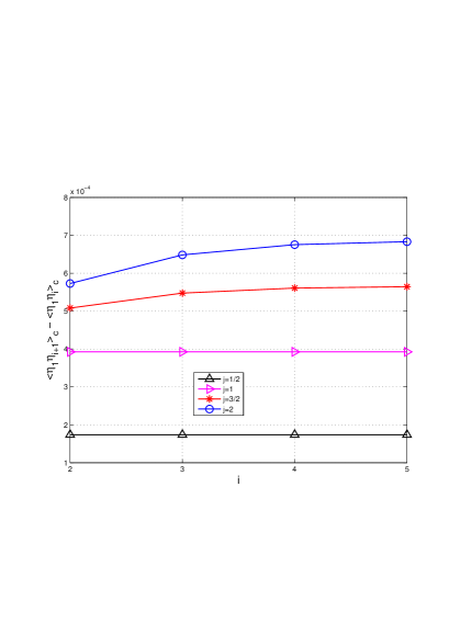
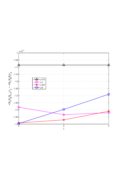
In this paragraph we provide the results of some numerical computations. We solved numerically the master equation for the invariant distribution of SEP() in the cases and and computed the correlations and . If were multilinear, the differences would be constant.
The simulations seem to confirm the bilinearity of the covariances in the cases (a) and (b) above, and the loss of bilinearity in the other cases. In Fig.1 (left panel) the values of are reported for the case : they are clearly constant for (case (a) above) and for (case (b) above) but not for and .
Concerning the 3-points correlations, the simulations show that the multilinearity is lost
even in the cases where it holds for (i.e. in the case (b)), while it
is conserved for the SEP(1) with at most one particle per site.
Figure 1 gives evidence for this phenomenon
by showing that are constant only for (case (a) above).
The deviation from multilinearity is in any case very small and, very likely, it is decreasing as increases.
7 Macroscopic fluctuation theory
The aim of this section is to show that the large scale properties of the models studied so far can be obtained by a suitable adaptation of the macroscopic fluctuation theory of [BDGJL, BDGJL1, BDGJL2, BDGJL3]. In particular we verify that the macroscopic limit of the exact solutions for the covariances found in Section 6 does match the prediction of the macroscopic fluctuation theory (see [DLS, DG] for the exclusion process with at most one particle per site).
7.1 Macroscopic fluctuation theory and density large deviations functional
We briefly review the approach of the macroscopic fluctuation theory. Let us consider a one dimensional diffusive systems of linear size in contact with two reservoirs at densities and . The macroscopic fluctuation theory describes the behavior of the system in the hydrodynamic limit in terms of the two quantities and , called diffusivity and mobility, defined by
| (7.1) | |||||
| (7.2) |
where
| (7.3) |
In the above equation is the total flow through the bond in the time interval , while is the instantaneous flow at time . The bracket denotes the expectation with respect to the stationary state for the system of size whose density on the left (resp. right) boundary is (resp. ).
From the macroscopic fluctuation theory [BDGJL2], we know that the probability of observing a time dependent density and current profiles and in a macroscopic time interval , under the diffusive scaling and , is , where is the action functional given by:
| (7.4) |
Then the probability of observing a density profile in the stationary state is where is the large deviation functional:
| (7.5) |
with the minimum in (7.5) taken over all the trajectories conditioned to the extreme values , the typical profile, and . Density and current must also satisfy the continuity equation
| (7.6) |
The density correlation functions in the stationary state can be obtained from the large deviation functional through the derivatives of its Legendre transform (see [D]):
| (7.7) |
Then, for large we have
| (7.8) | |||||
| (7.9) | |||||
7.2 From SEP(1) to models with constant diffusivity and quadratic mobility
In this section we use a scaling argument to deduce the density large deviations functional of a model with constant diffusivity and quadratic mobility from that of the SEP(1) (cfr. also [BDGJL2]). We start by recalling that for the SEP(1) one has
| (7.10) |
and therefore
| (7.11) |
then, from (7.5), one finds that the density large deviation functional is (see [DLS], [BDGJL3])
| (7.12) |
where the supremum is taken over the monotone functions with boundary values , . The supremum is attained for , monotone solution of the following differential problem:
| (7.13) |
The connected correlation functions can be obtained by computing the derivatives of the functional as in (7.7). One finds that the lowest order correlations are, for large ,
| (7.14) | |||||
for .
Let us now consider the generalization of (7.10) obtained by assuming that the diffusivity is constant and the mobility is a quadratic function parametrized as
| (7.15) |
where , and are given numbers. The action functional of this system
| (7.16) |
is related to through the following change of variables (cfr. [DG])
| (7.17) |
with
| (7.18) |
The scaling (7.17) has been chosen among all the possible scalings connecting and as it is the only one
preserving the conservation law (7.6) between and .
Then, by (7.17) and (7.5) it follows that
the large deviation functional for the system characterized by (7.15) is given by
| (7.19) |
and thus
with
| (7.21) |
where is the monotone function satisfying (7.13). Equivalently is the monotone solution of the differential problem
| (7.22) |
and, from (7.8) and (7.14), we have
| (7.24) | |||||
and, more generally, one gets a factor for the -point connected correlation function.
7.3 Macroscopic behavior of the correlations
With suitable choices of the parameters we can generate the large scale limits of models that we have considered in the previous sections.
Inclusion walkers SIP(). For interacting particle systems, the flux across bond in a time interval is given by the number of particles which jump from to minus the number of particles which jump from to . i.e.
| (7.25) | |||||
As a consequence, the expectation of the flow in the stationary state with boundary densities is given by
| (7.26) |
From Section 3.2 we know that the SIP() equilibrium stationary measure at density is the product of NegativeBinomial with a variance . Using (7.25)
| (7.27) |
Now we have
| (7.28) | |||||
where, in the last display, denotes the stationary equilibrium measure. By duality,
| (7.29) | |||||
where is the -dimensional configuration with and is the duality function defined in (4.10). Let be the transition probability from the site to the site in the time interval of a random walker on the set moving at rate , then
| (7.30) |
As a consequence (7.28) is equal to
| (7.31) |
where the two identities above follow from the product character of the equilibrium measure, and from the fact that depends only on the distance . Now the random walk is moving at rate , then, from the master equation we have
| (7.32) |
Then (7.3) is given by
| (7.33) |
Since vanishes as , we finally obtain, using (7.2) .
Summarizing, for the inclusion process SIP(), we have
| (7.34) |
which implies , and . This choice produces (see (7.24)) the following correlation functions:
| (7.35) |
where and are the SIP() boundary densities ( and in terms of our boundary parameters). Notice that the covariances in (7.3) do indeed agree with the macroscopic limit of the microscopic covariances that have been found in Section 6.1 (see (6.4)) for a particular choice of the parameters. Similarly, one gets for the density large deviation functional:
| (7.36) |
where is the monotone solution of
| (7.37) |
Exclusion walkers SEP(). The flux is now given by
| (7.38) | |||||
| (7.39) |
As a consequence, the expectation of with respect to the steady state measure reads
| (7.40) |
Thus, from (7.1) and (4.24), we get . From Section 3.2 we know that the SEP() stationary measure at density is the product of Binomial with a variance . Using a similar computation as for the inclusion walkers then, one can compute also the mobility, obtaining:
| (7.41) |
Therefore we have , , and, from (7.24), we have the following correlation functions:
| (7.42) |
where and are the SEP() boundary densities ( and in terms of our boundary parameters). The second line in (7.3) does agree with the microscopic SEP-covariances that have been found in Section 6.1 (see (6.8)) for a particular choice of the parameters. Moreover the density large deviation functional is given by
| (7.43) |
where is the monotone function satisfying
| (7.44) |
Independent random walkers IRW. As observed in [DG], the independent random walkers model, for which
| (7.45) |
is obtained in the limit as and . Under this choice, see (7.24), all the correlation functions vanish (this obviously reflects the fact that the stationary measure has a product structure, see Proposition 4.5). As , one can see from (7.2) that, due to the concavity of the logarithm, the derivative is constant. Therefore in this limit the optimal is given by
| (7.46) |
and one get
| (7.47) |
KMP model. The expectation of with respect to the steady state measure is now given by
| (7.48) | |||||
then, from (7.1) and (4.26), we get . We know that the KMP stationary measure at temperature is the product of Exponential. By a duality argument we compute also the mobility and get
| (7.49) |
The KMP model can be, then, obtained (see [DG]) by taking the unphysical limit , with . In this limit the first three connected correlations functions (see 7.24) are
| (7.50) |
which agree with (2.38) of [BDGJL]. Moreover the density large deviation functional that we obtain
| (7.51) |
agrees with the same function computed in [BGL].
Acknowledgments. We are extremely grateful to Bernard Derrida, with whom we discussed some of the topics in this work. In particular we own to him the results of Section 7 for the comparison to macroscopic fluctuation theory.
We acknowledge financial support from the by the Italian Research Funding Agency (MIUR) through FIRB project “Stochastic processes in interacting particle systems: duality, metastability and their applications”, grant n. RBFR10N90W and the Fondazione Cassa di Risparmio Modena through the International Research 2010 project.
8 Appendix: Equations for the two points correlations
We provide the linear systems that must be satisfied by
the two points correlation functions in the steady state, i.e.
with .
In the following, equations 1),2),3) are obtained by letting act the generator on a couple
of sites at distance larger or equal than two,
equations 4),5),6) are derived from nearest-neighbouring sites,
equations 7),8),9) correspond to the diagonal,
equation 10) is obtained from the couple (1,L).
Inclusion/Exclusion walkers: the equations for the inclusion walkers SIP() and for the exclusion walkers SEP()
are similar, with some relevant change of signs in the two cases; therefore we write them
together. With the convention to use upper symbol for inclusion and lower symbol for exclusion
in and and with the further convention that for SIP() and for SEP(),
the equations read
Brownian energy process BEP(): the equations for the BEP() read
References
- [BD] T. Bodineau, B. Derrida, “Current fluctuations in nonequilibrium diffusive systems: an additivity principle”, Phys. Rev. Lett. 92 (18),180601 (2004).
- [BDGJL] L.Bertini, A. De Sole, D. Gabrielli, G. Jona-Lasinio, C. Landim, “Stochastic interacting particle systems out of equilibrium”, J.Stat.Mech. P07014 (2007)
- [BDGJL1] L.Bertini, A. De Sole, D. Gabrielli, G. Jona-Lasinio, C. Landim, “Non equilibrium current fluctuations in stochastic lattice gases”, J.Stat.Phys. 123, 237–276, (2006).
- [BDGJL2] L. Bertini, A. De Sole, D. Gabrielli, G. Jona-Lasinio, C. Landim, “Large deviation approach to non equilibrium processes in stochastic lattice gases ”, Bull. Braz. Math. Soc., New Series 37 (4), 611–643, (2006).
- [BDGJL3] L. Bertini, A. De Sole, D. Gabrielli, G. Jona-Lasinio, C. Landim, “Large deviations for the boundary driven symmetric simple exclusion process”, Mathematical Physics, Analysis and Geometry 6, (3), 231–267 (2003).
- [BGL] L.Bertini, D. Gabrielli, J. Lebowitz, “Large deviations for a stochastic model of heat flow ”, J. Stat. Phys., Vol. 121, N. 5/6, 843-885, (2005).
- [BO] C. Bernardin, S. Olla, “Fourier’s law for a microscopic model of heat conduction ”, J. Stat. Phys. 121 , 271-289, (2005).
- [BCS] A. Borodin, I. Corwin, T. Sasamoto From duality to determinants for q-TASEP and ASEP preprint http://arxiv.org/abs/1207.5035 (2013).
- [CGGR] G. Carinci, C. Giardinà, C. Giberti, F. Redig, “Dualities in population genetics: a fresh look with new dualities”, preprint http://arxiv.org/abs/1302.3206 (2013).
- [D] B. Derrida, “Non-equilibrium steady states: fluctuations and large deviations of the density and of the current”, J. Stat. Mech. P07023 (2007).
- [DE] B. Derrida, M.R. Evans, “Exact correlation functions in an asymmetric exclusion model with open boundaries”, J. Phys. I France 3, 311-322 (1993).
- [DEHP] B. Derrida, M.R. Evans, V. Hakim, V. Pasquier, “Exact solution of a 1d asymmetric exclusion model using a matrix formulation”, J. Phys. A26, 1493-1517 (1993).
- [DG] B. Derrida, A.Gerschenfeld, “Current fluctuations in one dimensional diffusive system with a step initial profile”, J. Stat. Phys., Vol. 137, N. 5-6, 978-1000, (2009).
- [DL] D. Dolgopyat, C. Liverani, Energy transfer in a fast-slow Hamiltonian system, Comm. Math. Phys. 308, (1), 201–225, (2011).
- [DLS] B. Derrida, J.L. Lebowitz, E.R. Speer, “Large deviation of the density profile in the steady state of the open symmetric simple exclusion process”, J. Stat. Phys., Vol. 107, N. 3/4, 599-634, (2002).
- [DLS1] B. Derrida, J.L. Lebowitz, E.R. Speer, “Entropy of open lattice systems”, J. Stat. Phys., Vol. 126, N. 4/5, 1083-1108, (2007).
- [GC] G. Gallavotti, E.G.D. Cohen, “Dynamical ensembles in nonequilibrium statistical mechanics”, Phys. Rev. Lett. 74, 2694-2697 (1995); “Dynamical ensembles in stationary states”, J. Stat. Phys. 80, 931-970, (1995).
- [GK] C. Giardinà, J. Kurchan, “Fourier law in a momentum conserving chain”, J. Stat. Mech., P05009, (2005).
- [GKLT] C. Giardinà, J. Kurchan, V. Lecomte, J. Tailleur, “Simulating rare events in dynamical processes”, J. Stat. Phys. 145 (4) 787–811 (2011).
- [GKR] C. Giardinà, J. Kurchan, F. Redig, “Duality and exact correlations for a model of heat conduction”, J. Math. Phys. 48, 033301 (2007).
- [GKRV] C. Giardinà, J. Kurchan, F. Redig, K. Vafayi, “Duality and hidden symmetries in interacting particle systems”, J. Stat. Phys. 135 , 25-55, (2009).
- [GRV] C. Giardinà, F. Redig, K. Vafayi, “Correlation Inequalities for interacting particle systems with duality”, J. Stat. Phys., Vol.141, No. 2, 242-263 (2010).
- [GRV2] S. Grosskinsky,F. Redig, K. Vafayi, “Condensation in the inclusion process and related models”, J. Stat. Phys. 142 (5), 952–974, (2011).
- [JK] S. Jansen, N. Kurt, “On the notion(s) of duality for Markov processes”, preprint arXiv:1210.7193.
- [K] J. Kurchan, “The fluctuation theorem for stochastic dynamics”, J.Phys.A: Math. Gen. 31 3719 (1998).
- [KMP] C. Kipnis, C. Marchioro, E. Presutti, “Heat flow in an exactly solvable model”, J. Stat. Phys. 27(1), 65–74 (1982).
- [Keis] J.D. Keisling, “An ergodic theorem for the symmetric generalized exclusion process”, Markov Process. Related Fields 4, 351–379 (1998).
- [LAW] V. Lecomte, C. Appert-Rolland, F. van Wijland, “Thermodynamic formalism for systems with Markov dynamics”, J. Stat. Phys. 127, 51–106 (2007).
- [LMS] E. Levine, D. Mukamel, G. M. Schütz, “Zero range process with open boundaries”, J. Stat. Phys. 120, 759–778 (2005).
- [L] T. M. Liggett, “Interacting particle systems”, Springer, (1985).
- [S] F. Spitzer, “Interaction of Markov processes”, Adv. Math. 5, 246-290, (1970).
- [Spo] H. Spohn, “Long range correlations for stochastic lattice gases in a non-equilibrium steady state”, J.Phys.A: Math. Gen. 16, 4275-4291 (1983).
- [SS] G. Schütz, S. Sandow, “Non-Abelian symmetries of stochastic processes: Derivation of correlation functions for random-vertex models and disordered-interacting-particle systems”, Phys. Rev. E 49, 2726 (1994).