Large sets of consecutive Maass forms and fluctuations in the Weyl remainder

Abstract.

We explore an algorithm which systematically finds all discrete eigenvalues of an analytic eigenvalue problem. The algorithm is more simple and elementary as could be expected before. It consists of Hejhal’s identity, linearisation, and Turing bounds. Using the algorithm, we compute more than one hundredsixty thousand consecutive eigenvalues of the Laplacian on the modular surface, and investigate the asymptotic and statistic properties of the fluctuations in the Weyl remainder. We summarize the findings in two conjectures. One is on the maximum size of the Weyl remainder, and the other is on the distribution of a suitably scaled version of the Weyl remainder.

1. Introduction

The real-analytic eigenvalue problem of the Laplacian on finite, non-compact hyperbolic surfaces is an important one. The solutions are automorphic forms and play a central role in analytic number theory. They can be used to extend the classical theory of Dirichlet series with Euler products [21] and are closely related to the Millennium Problem of the Riemann Hypothesis [29]. Moreover, they serve to find class numbers of real quadratic number fields and hence solve questions which already inspired Gauss [5]. Non-holomorphic automorphic forms, the so called Maass forms, are intensively studied in spectral theory. The spectral decomposition into Maass forms let to the discovery of Selberg’s trace formula [30, 11] which connects the spectrum to the geometric properties of the underlying space. Automorphic forms are the prime example of quantum unique ergodicity [20]. In addition, Maass forms span a Hilbert basis in quantum mechanics on hyperbolic surfaces and serve as important examples in quantum chaos. For instance, they play a distinguished role in eigenvalue statistics [2, 3]. As a complete set of eigenfunctions of the Laplacian on hyperbolic surfaces they have also found applications in general relativity and cosmology [1].

By approximating them, numerics can bring Maass forms closer to us [16]. It is clear how to compute Maass forms [13]. However, it was difficult to find consecutive sets of solutions. We present an algorithm which allows us to find large consecutive sets of Maass forms efficiently. The algorithm is based on three ingredients: Hejhal’s identity to compute eigenfunctions corresponding to given eigenvalues; linearisation which converts the analytic eigenvalue problem locally to a matrix eigenvalue problem; and explicit Turing bounds which serve to check and complete the results.

As they lie on our route, we apply results of ergodic theory, namely the equidistribution of long closed horocycles [34, 28, 12, 14, 10, 32]. This allows us to unreveil an elegant view on the derivation of Hejhal’s identity in section 4, where we present the computation of Maass forms under the preliminary assumption that the discrete eigenvalues would be known. The eigenvalue problem is linearised in section 5, thereby almost all of the eigenvalues are found. Section 6 presents Turing bounds. These bounds drive a control algorithm which systematically checks and completes the list of Maass forms until a large set of consecutive Maass forms is found. We have computed more than $160\,000$ consecutive Maass forms. This exceeds any previous numerical solution of any non-integrable system by far. Results are listed in section 7, where we investigate the asymptotic and statistic properties of the fluctuations in the Weyl remainder.

2. Fundamental domains, equidistribution of long closed horocycles, and congruent points

In this section, we will consider fundamental domains, present a pullback algorithm, and use ergodic properties to show that a discrete subgroup of the isometries can be completely specified by a set of congruent pairs of points.

Let $X=\Gamma\backslash\mathcal{H}$ be a surface, where $\Gamma$ is a cofinite, non-cocompact subgroup of $\operatorname{SL}(2,\mathbb{R})$ which acts properly discontinuous on the Poincaré upper half-plane $\mathcal{H}$. The action is given by linear fractional transformations. On $X$ we have the invariant metric $ds=|dz|/y$. We use $\ell(\cdot)$ to denote length, and $d(\cdot,\cdot)$ to denote hyperbolic distance.

Because $\Gamma$ is non-cocompact, $X$ has at least one cusp. After a suitable coordinate transformation we may assume that one of the cusps lies at $\infty$, and that the corresponding isotropy subgroup $\Gamma_{\infty}\subset\Gamma$ is generated by $z\mapsto z+1$.

Take some point $p$ in $\mathcal{H}$, not an elliptic fixed point. Let $\mathcal{F}$ be the corresponding Dirichlet fundamental domain:

$$\mathcal{F}=\{z\in\mathcal{H}\ |\ d(p,z)\leq d(p,\gamma z)\ \forall\gamma\in\Gamma\}.$$

We know from Siegel’s theorem that $\mathcal{F}$ has a finite number of sides. The sides of $\mathcal{F}$ fall into congruent pairs, let us denote them $s_{1},s_{n+1};s_{2},s_{n+2};\ldots;s_{n},s_{2n}$, and let $g_{1},g_{2},\ldots,g_{n}\in\Gamma$ be the identification maps, $g_{k}s_{k}=s_{n+k}$. (Recall the convention that an elliptic fixed point of order two is considered as a vertex separating two distinct sides of $\mathcal{F}$.) We know that $g_{1},g_{2},\ldots,g_{n}$ generate $\Gamma$ (see [18, pp. 73–74]).

The following is an algorithm for computing the pullback of any given point in the hyperbolic plane into a Dirichlet fundamental domain.

Algorithm 1 (Pullback algorithm [31]).

1. Start with $z\in\mathcal{H}$.

2. Compute the $2n$ points $g_{1}z,g_{1}^{-1}z,g_{2}z,g_{2}^{-1}z,\ldots,g_{n}^{-1}z$. Let $z^{\prime}$ be the one of these which has smallest hyperbolic distance to $p$.

3. If $d(p,z^{\prime})<d(p,z)$, then replace $z$ by $z^{\prime}$, and repeat from 2.

4. In the other case, $d(p,z^{\prime})\geq d(p,z)$, we know that $z$ lies in $\mathcal{F}$, hence $z$ is the searched-for pullback.

Strömbergsson proved that his pullback algorithm always finds the pullback within a finite number of operations [31].

We use $z^{*}=x^{*}+iy^{*}$ to denote the pullback of $z=x+iy$, and $\mathcal{A}^{*}=\{z^{*}\ |\ z\in\mathcal{A}\}$ to denote the pullback of $\mathcal{A}$, for any $\mathcal{A}\subseteq\mathcal{H}$.

For any $y>0$, the curve $L_{y}=\{x+iy\ |\ x\in[0,1]\}$ is a closed horocycle of length $\ell=1/y$ on $X$. When $\ell\to\infty$, this curve is known to become uniformly equidistributed on $X$ with respect to the Poincaré area $d\mu=dxdy/y^{2}$ [32]. Let us consider $Q$ equidistant points $\{z_{j}\}_{1\leq j\leq Q}$ on the closed horocyle $L_{y}$. Using Algorithm 1, we can compute $\{z_{j}^{*}\}_{1\leq j\leq Q}$, and construct the congruent pairs of points $\{(z_{j},z_{j}^{*})\}_{1\leq j\leq Q}$.

Of importance is:

Lemma 2.

Fix $Q\in\mathbb{N}$ and $y>0$, and consider $Q$ equidistant points $\{z_{j}\}_{1\leq j\leq Q}$ on the closed horocycle $L_{y}$. For $Q$ sufficiently large and $y$ sufficiently small, the congruent pairs of points $\{(z_{j},z_{j}^{*})\}_{1\leq j\leq Q}$ contain all information of the group $\Gamma$.

For $\mathcal{A}\subseteq\mathcal{H}$, we use $\partial\mathcal{A}$ to denote its boundary, and $\Gamma\mathcal{A}=\{\gamma z\ |\ z\in\mathcal{A},\gamma\in\Gamma\}$ to denote its orbit.

For the proof of Lemma 2, we need the following:

Lemma 3.

If the horocycle $L_{y}^{*}$ comes sufficiently close to each point in $\mathcal{F}$, then we have: For each $1\leq k\leq n$ there exists a line segment $l_{k}\subset L_{y}$ such that $l_{k}$ meets $\Gamma\partial\mathcal{F}$ exactly once, $l_{k}^{*}$ does not meet $\partial\mathcal{F}$ in a vertex, and $\ell(l_{k})>\ell(l_{k}\cap\gamma_{k}^{-1}\mathcal{F})>0$ for some $\gamma_{k}\in\Gamma$.

Proof.

Fix $1\leq k\leq n$. Fix some point $\omega_{k}\in s_{k}$, not a vertex of $\mathcal{F}$. By assumption $L_{y}^{*}$ comes sufficiently close to any point in $\mathcal{F}$. Thus, for some $\varepsilon>0$ there exists $\gamma_{k}\in\Gamma$ such that $|y-\Im(\gamma_{k}^{-1}\omega_{k})|<\varepsilon$. If unexpectedly $\Im(\gamma_{k}^{-1}\omega_{k})=\sup_{\omega\in s_{k}}\Im(\gamma_{k}^{-1}\omega)$ should hold, we repeat the proof with another $\omega_{k}\in s_{k}$.

We have $\inf_{\omega\in s_{k}}\Im(\gamma_{k}^{-1}\omega)<\Im(\gamma_{k}^{-1}\omega_{k})<y+\varepsilon$ and $y-\varepsilon<\Im(\gamma_{k}^{-1}\omega_{k})<\sup_{\omega\in s_{k}}\Im(\gamma_{k}^{-1}\omega)$. For $\varepsilon$ sufficiently small, $L_{y}$ intersects $\gamma_{k}^{-1}s_{k}$ at least once (and at most twice) not at a vertex.

Take an open line segment $l_{k}\subset L_{y}$ such that $l_{k}$ intersects $\gamma_{k}^{-1}s_{k}$, and such that it meets $\Gamma\partial\mathcal{F}$ exactly once, but not in a vertex of $\gamma_{k}^{-1}\mathcal{F}$. Since $l_{k}$ is an open line segment, it has positive length on both sides of the intersection with $\gamma_{k}^{-1}s_{k}$. ∎

Proof of Lemma 2.

Our task is to extract the side identification maps $g_{1},\ldots,g_{n}$ from the pairs of points $\{(z_{j},z_{j}^{*})\}_{1\leq j\leq Q}$.

The points $z_{1},\ldots,z_{Q}$ are on the curve $L_{y}$. In the limit $y\to 0$, the closed horocycle $L_{y}$ equidistributes on $\Gamma\backslash\mathcal{H}$. If $y>0$ is finite, the curve $L_{y}^{*}$ is no longer dense in $\mathcal{F}$. Still, for $y$ sufficiently small, $L_{y}^{*}$ comes sufficiently close to each point in $\mathcal{F}$.

Fix some $1\leq k\leq n$. Let $l_{k}$ be the line segment given by Lemma 3. There are two distinct elements $\gamma_{k}$,$\gamma_{n+k}\in\Gamma$, $\gamma_{k}\not=\pm\gamma_{n+k}$, such that $\ell(l_{k}\cap\gamma_{k}^{-1}\mathcal{F})>0$ and $\ell(l_{k}\cap\gamma_{n+k}^{-1}\mathcal{F})>0$. For $Q$ sufficiently large, at least three succesive points of $\{z_{j}\}_{1\leq j\leq Q}$ are on $l_{k}\cap\gamma_{k}^{-1}\mathcal{F}$ and another three are on $l_{k}\cap\gamma_{n+k}^{-1}\mathcal{F}$. This is true for any $1\leq k\leq n$. Hence, for each $1\leq k\leq n$ there are six succesive pairs of points in $\{(z_{j},z_{j}^{*})\}_{1\leq j\leq Q}$ such that three of them satisfy $z_{j}^{*}=\gamma_{k}z_{j}$, while the other three satisfy $z_{j}^{*}=\gamma_{n+k}z_{j}$.

Now, let only the congruent pairs of points $\{(z_{j},z_{j}^{*})\}_{1\leq j\leq Q}$ be given. We search for all sequences of six succesive pairs of points in $\{(z_{j},z_{j}^{*})\}_{1\leq j\leq Q}$ subject to the condition that three of them satisfy $z_{j}^{*}=\gamma_{h}z_{j}$, while the other three of them satisfy $z_{j}^{*}=\gamma_{h^{\prime}}z_{j}$, where $\gamma_{h},\gamma_{h^{\prime}}\in\operatorname{SL}(2,R)$, $\gamma_{h}\not=\pm\gamma_{h^{\prime}}$. By construction all $\gamma_{h}$ and $\gamma_{h^{\prime}}$ are in $\Gamma$. Moreover, amongst all these sequences of six succesive pairs of points, for each $1\leq k\leq n$ there is at least one sequence which is associated to the congruent pair of sides $s_{k},s_{n+k}$. The corresponding side identification map (or its inverse) follows from $g_{k}=\gamma_{h}\gamma_{h^{\prime}}^{-1}$. ∎

3. Maass forms

Let $X=\Gamma\backslash\mathcal{H}$ be a finite, non-compact surface with invariant metric $ds=|dz|/y$. According to the metric, the Laplacian reads $\Delta=-y^{2}(\partial^{2}/\partial x^{2}+\partial^{2}/\partial y^{2})$.

Definition 4 ([21]).

A Maass form is a

1. real analytic, $f\in C^{\infty}(\mathcal{H})$,

2. square integrable, $f\in L^{2}(X)$,

3. automorphic, $f(\gamma z)=f(z)\ \forall\gamma\in\Gamma$,

4. eigenfunction of the Laplacian, $\Delta f(z)=\lambda f(z)$.

If a non-constant Maass form vanishes in all cusps of $X$, it is called a Maass cusp form.

According to the Roelcke-Selberg spectral resolution of the Laplacian [30, 24], its spectrum contains both, a discrete and a continuous part. The discrete part of the spectrum is spanned by the constant eigenfunction $f_{0}$ and a countable number of Maass cusp forms $f_{1},f_{2},f_{3},\ldots$ which we take to be ordered with increasing eigenvalues $0=\lambda_{0}<\lambda_{1}\leq\lambda_{2}\leq\lambda_{3}\leq\ldots$. The continuous part of the spectrum $\lambda\geq 1/4$, is spanned by Eisenstein series.

In order to keep notation simple, we focus on Maass cusp forms on finite surfaces with exactly one cusp. We assume that the cusps lies at $\infty$, and that the corresponding isotropy subgroup $\Gamma_{\infty}\subset\Gamma$ is generated by $z\mapsto z+1$.

In this setting, Maass cusp forms associated to the eigenvalue $\lambda=r^{2}+1/4$ have the Fourier expansion

$$f(z)=\sum_{n\in\mathbb{Z}-\{0\}}a_{n}y^{1/2}K_{ir}(2\pi|n|y)e^{2\pi inx},$$

where $K$ stands for the $K$-Bessel function which decays exponentially for large arguments [7, Eq. (14)]. The expansion coefficients $a_{n}$ grow at most polynomially in $n$. If we bound $y$ from below, $y\geq Y$, and allow for a small numerical error of size $\varepsilon>0$, there is an $M(Y)=const/Y$ such that

(1) $$f(z)=\sum_{0\not=|n|\leq M(Y)}a_{n}y^{1/2}K_{ir}(2\pi|n|y)e^{2\pi inx}+[|error|<\varepsilon].$$

The constant in $M(Y)=const/Y$, which depends on $\varepsilon>0$, $r$, and the group $\Gamma$, can be worked out explicitly in each case. Of importance is:

Lemma 5.

Let the fundamental domain $\mathcal{F}$ be bounded from below, $Y_{0}:=\inf_{z\in\mathcal{F}}\Im(z)>0$. Apart from a numerical error of at most $\varepsilon>0$, a Maass cusp form is completely specified by its eigenvalue and a finite number of expansion coefficients, $\{\lambda,\{a_{n}\}\}_{0\not=|n|\leq M(Y_{0})}$.

Proof.

Let $\{\lambda,\{a_{n}\}\}_{0\not=|n|\leq M(Y_{0})}$ be given. By automorphy it is enough to know $f(z)$ inside the fundamental domain. There, we have $y\geq Y_{0}$, and the value of $f(z)$ follows from (1). ∎

Remark 6.

For any $\{\lambda,\{a_{n}\}\}_{0\not=|n|\leq M(Y_{0})}$, the Fourier expansion (1) is real analytic, square integrable on $X$, vanishes in the cusp at $\infty$, and satisfies the eigenvalue equation of the Laplacian. However, only for very specific choices of $\{\lambda,\{a_{n}\}\}_{0\not=|n|\leq M(Y_{0})}$, the corresponding function is automorphic, and hence a Maass cusp form.

4. Computing Maass forms

For the moment, we assume that the eigenvalue would be given. Our task is to find the coefficients $\{a_{n}\}$ such that automorphy holds, $f(\gamma z)=f(z)\ \forall\gamma\in\Gamma$. We use the congruent pairs of points of Lemma 2 with $0<y<Y_{0}$ and $Q\geq 2M(y)$ to test automorphy, $f(z_{j}^{*})=f(z_{j})$ for all $1\leq j\leq Q$. This results in $Q$ linear equations in $2M$ unknowns $\{a_{n}\}_{0\not=|n|\leq M}$.

Note, however, that $f(z_{j})=f(z_{j}^{*})$ is ill-conditioned. If one tries to solve for $a_{M}$, one gets $a_{M}y^{1/2}K_{ir}(2\pi|M|y)e^{2\pi iMx_{j}}=f(z_{j}^{*})-[f(z_{j})_{\text{less the $M$-th summand}}]$. The absolute value of the l.h.s is bounded by $\varepsilon$ which is smaller than the numerical error of the r.h.s..

We use exponentially weighted superpositions to convert the ill-conditioned linear system of equations into a well-conditioned linear system of equations [13],

$$\frac{1}{Q}\sum_{j=1}^{Q}f(z_{j})e^{-2\pi imx_{j}}=\frac{1}{Q}\sum_{j=1}^{Q}f(z_{j}^{*})e^{-2\pi imx_{j}}.$$

Using geometric series on the l.h.s. and Fourier expanding the r.h.s. results in Hejhal’s identity:

(2) $$a_{m}y^{1/2}K_{ir}(2\pi|m|y)+[|error|<\varepsilon]=\frac{1}{Q}\sum_{j=1}^{Q}f(z_{j})e^{-2\pi imx_{j}}\\ =\frac{1}{Q}\sum_{j=1}^{Q}f(z_{j}^{*})e^{-2\pi imx_{j}}=\sum_{0\not=|n|\leq M(Y_{0})}a_{n}V_{mn}+[|error|<\varepsilon]\qquad\forall 0\not=|m|\leq M(y)$$

where $V_{mn}=\frac{1}{Q}\sum_{j=1}^{Q}{y_{j}^{*}}^{1/2}K_{ir}(2\pi|n|y_{j}^{*})e^{2\pi i(nx_{j}^{*}-mx_{j})}$.

Algorithm 7 (Phase 2 [13]).

If $\{\lambda,\{a_{n}\}\}_{0\not=|n|\leq M(Y_{0})}$ are given, then any further coefficients follow directly from

$$a_{m}\simeq\frac{1}{y^{1/2}K_{ir}(2\pi|m|y)}\sum_{0\not=|n|\leq M(Y_{0})}V_{mn}a_{n}\qquad\forall|m|>M(Y_{0})$$

as $y\to 0$. The numerical error is bounded by

$$|error\text{ of }a_{m}|<\frac{2\varepsilon}{|y^{1/2}K_{ir}(2\pi|m|y)|}.$$

We use $C(\lambda)$ to denote the matrix $C_{mn}(\lambda)=\delta_{mn}-\frac{V_{mn}}{y^{1/2}K_{ir}(2\pi|m|y)}$, $0\not=|m|\leq M(Y_{0})$, $0\not=|n|\leq M(Y_{0})$, and $\vec{a}$ to denote the vector $\vec{a}=(a_{-M(Y_{0})},a_{-M(Y_{0})+1},\ldots,a_{-1},a_{1},a_{2},\ldots,a_{M(Y_{0})})$.

Algorithm 8 (Phase 1 [13]).

If only $\lambda$ is given, then the coefficients $\{a_{n}\}_{0\not=|n|\leq M(Y_{0})}$ follow from solving the linear system of equations

$$C(\lambda)\vec{a}\simeq 0,\qquad\vec{a}\not=0.$$

The numerical error is bounded by

$$\Big{|}error\text{ of }\sum_{0\not=|n|\leq M(Y_{0})}C_{mn}a_{n}\Big{|}<\frac{2\varepsilon}{|y^{1/2}K_{ir}(2\pi|m|y)|}\qquad\forall 0\not=|m|\leq M(Y_{0}).$$

Remark 9.

If we make a good choice for the height $y$ of the horocycle and take some $M_{0}\geq M(Y_{0})$ such that $|y^{1/2}K_{ir}(2\pi|m|y)|\gg 1$ for all $0\not=|m|\leq M_{0}$, the linear system of equations (2) is well-conditioned for $0\not=|m|\leq M_{0}$.

5. Finding eigenvalues

It remains to find the eigenvalues $\lambda$ for which the linear system $C(\lambda)\vec{a}\simeq 0$ has non-trivial solutions $\vec{a}\not=0$, and for which the non-trivial solutions are independent of the height $y$ of the horocycle.

To this end, we discretise the $\lambda$-axis into trial values $0<\tilde{\lambda}_{1}<\tilde{\lambda}_{2}<\tilde{\lambda}_{3}<\ldots$ which lie sufficiently close together, and explore the neighbourhood of each trial value for non-trivial solutions of $C(\tilde{\lambda}+h)\vec{a}\simeq 0$. For the latter, we linearise with respect to the eigenvalue, cf. [27],

$$C(\tilde{\lambda}+h)=C(\tilde{\lambda})+hC^{\prime}(\tilde{\lambda})+\frac{h^{2}}{2}R(\tilde{\lambda},h),$$

where $R(\tilde{\lambda},h)$ is a matrix whose norm is bounded by

$$||R(\tilde{\lambda},h)||\leq\sup_{|\xi|\leq|h|}||C^{\prime\prime}(\tilde{\lambda}+h)||.$$

Let $\tilde{\lambda}$ be fixed, $\eta$ be a small complex parameter, and let $(h_{\eta},\vec{\alpha}_{\eta})_{|\tilde{\lambda}}$ be the non-trivial solutions of

(3) $${C^{\prime}}^{-1}(\tilde{\lambda})\big{(}C(\tilde{\lambda})+\frac{\eta^{2}}{2}R(\tilde{\lambda},\eta)\big{)}\vec{\alpha}_{\eta}=-h_{\eta}\vec{\alpha}_{\eta}.$$

For $\eta=0$, we know $(h,\vec{\alpha})_{|\tilde{\lambda}}:=(h_{0},\vec{\alpha}_{0})_{|\tilde{\lambda}}$ numerically. If $C^{\prime}(\tilde{\lambda})$ is regular, there are $2M(Y_{0})$ matrix eigenvalues of ${C^{\prime}}^{-1}(\tilde{\lambda})C(\tilde{\lambda})$, and there are $2M(Y_{0})$ generalized eigenvectors.

For $\eta\not=0$, we use perturbation theory to find $(h_{\eta},\vec{\alpha}_{\eta})_{|\tilde{\lambda}}$.

Conjecture 10.

Under suitable conditions, in particular $|\eta|$ sufficiently small, we have

$$h_{\eta}=h+O(\eta^{2})\quad\text{and}\quad\vec{\alpha}_{\eta}=\vec{\alpha}+O(\eta).$$

Apart from numerical confirmations, it would be nice to have a proof of Conjecture 10. However, it is not even evident that all solutions of (3) have a Taylor expansion in $\eta$ around $0$.

If Conjecture 10 is true, it implies the following: Using $\eta=h_{\eta}$ in (3), we get $C(\tilde{\lambda}+\eta)\alpha_{\eta}=0$ with $\eta=h+O(\eta^{2})$ and $\vec{\alpha}_{\eta}=\vec{\alpha}+O(\eta)$. For $|\eta|$ sufficiently small this can be solved for $\eta$ which gives $\eta=h+O(h^{2})$. This allows to find numerical approximations, $\lambda=\tilde{\lambda}+h+O(h^{2})$, for the eigenvalues of $C(\lambda)\vec{a}\simeq 0$ in some neighbourhood of the trial value $\tilde{\lambda}$. The approximations can be refined iteratively. This establishes:

Theorem 11.

If Conjecture 10 holds true, and if the trial values $0<\tilde{\lambda}_{1}<\tilde{\lambda}_{2}<\ldots<\tilde{\lambda}_{\text{max}}$ lie sufficiently close together, the linearisation in the eigenvalue allows to find all eigenvalues of $C(\lambda)\vec{a}\simeq 0$ in the interval $[0,\tilde{\lambda}_{\text{max}}]$.

Remark 12.

1. Not each solution of $\big{(}{C^{\prime}}^{-1}(\tilde{\lambda})C(\tilde{\lambda})+hI\big{)}\vec{\alpha}=0$ approximates a Maass form. Clearly, $|h|$ can be too large such that the linearisation becomes inappropriate. This is of no concern, since we do not need to consider Maass forms whose eigenvalues are further away than the next trial value $\tilde{\lambda}$.

2. It can happen that a formal solution is dependent on $y$. This has to be checked explicitly by re-evaluating $C(\lambda)\vec{a}$ for different heights $y$ of the horocycle. Only if $C(\lambda)\vec{a}\simeq 0$ holds for all $0<y<Y_{0}$, we have found a Maass cusp form. Typically, it is enough to (re-)evaluate for a few different, but well chosen values of $y$.

3. The Laplacian on $X$ is an essentially self-adjoint operator. Hence, all eigenvalues $\lambda$ are real. Note, however, that the matrix $C(\tilde{\lambda})$ is not hermite by construction. As such there is no guarantee that the linearisation of $C(\tilde{\lambda}+h)\vec{a}\simeq 0$ results in real solutions. But, if it turns out that a solution becomes independent of $y$ then the eigenvalue $\lambda=\tilde{\lambda}+h+O(h^{2})$ becomes real, and the Maass form can be made real.

4. It may happen that there is no eigenvalue $\lambda$ near a trial value $\tilde{\lambda}$. In this case, there are still $2M(Y_{0})$ formal solutions of $\big{(}{C^{\prime}}^{-1}(\tilde{\lambda})C(\tilde{\lambda})+hI\big{)}\vec{\alpha}=0$, but $|h|$ is too large, or the formal solutions depend on the height $y$ of the horocycle.

5. According to Remark 9, a good choice for the height $y$ of the horocycle is cruical. In addition, we have to take care that $C^{\prime}(\tilde{\lambda})$ is regular and well-conditioned. However, it is hard to predict a good value for the height $y$ of the horocycle in advance. Moreover, a good choice of $y$ depends on $\lambda$.

   We fix some reasonable value of $y$ and search with this value of $y$ for Maass forms. Sometimes, our choice of $y$ may be good, and sometimes not. Whenever the choice of $y$ is not good, we may miss Maass forms. We compensate for this by taking another reasonable value of $y$ and run the algorithm again.

6. It may happen that eigenvalues degenerate. In principle, this is no problem for our algorithm. However, the speed of numerical convergence and the numerically implied errors are strongly affected. Whenever a degenerated eigenvalue occurs, a good choice for the height $y$ of the horocycle becomes even more important.

7. One may argue that Maass cusp forms, if completely desymmetrised, are conjectured to be non-degenerated. However, the algorithm does not distinguish whether a degeneracy happens between Maass cusp forms, or whether the degeneracy is between a Maass cusp form and another formal solution of $\big{(}{C^{\prime}}^{-1}(\tilde{\lambda})C(\tilde{\lambda})+hI\big{)}\vec{\alpha}=0$. In particular, degeneracies with formal solutions happen frequently.

8. In order to speed up the numerics, we do not take the trial values $0<\tilde{\lambda}_{1}<\tilde{\lambda}_{2}<\ldots<\tilde{\lambda}_{\text{max}}$ to be sufficiently close together, and hence intentionally risk to oversee solutions. We compensate for this by using Weyl’s average law and Turing bounds after the fact to figure out whether eigenvalues have been overseen. Any missing eigenvalues are eventually found with the aid of Algorithm 18.

9. For each trial value $\tilde{\lambda}$, we search for Maass forms in a neighbourhood. The neighbourhoods may overlap. Additionally, we may re-run the algorithm. For this reason, we typically find each Maass form more than once. Whenever we find a Maass form, we consider it only, if it does not match any previously found Maass form.

6. Turing bound

From Remark 12(5) and 12(8) it is obvious that we may miss some eigenvalues. In the current section, we use average Weyl’s law and Turing bounds to detect whether eigenvalues have been missed, and to figure out small intervals where the missing eigenvalues are to be found.

Let $\mathcal{N}(t)=\#\{\lambda\ |\ 1/4\leq\lambda\leq t^{2}+1/4\}$ count the number of eigenvalues which fall into the interval $[1/4,t^{2}+1/4]$. Average Weyl’s law reads

$$\mathcal{N}(t)=\mathcal{M}(t)+S(t),$$

where $\mathcal{M}(t)$ is a smooth approximation to $\mathcal{N}(t)$ such that the average value of the Weyl remainder $S(t)$ becomes zero in the limit $t\to\infty$,

$$\langle S(t)\rangle:=\frac{1}{t}\int_{0}^{t}S(\tau)d\tau\overset{t\to\infty}{\longrightarrow}0.$$

For Maass forms on certain hyperbolic surfaces, average Weyl’s law has been derived explicitly [6, 17]. An important example is Weyl’s average law on the modular surface.

Theorem 13 (Average Weyl’s law on the modular surface [6]).

On the modular surface $X=\operatorname{SL}(2,\mathbb{Z})\backslash\mathcal{H}$ we have for $t>0$:

$$\mathcal{M}(t)=\frac{1}{12}t^{2}-\frac{2t}{\pi}\log\frac{t}{e\sqrt{\pi/2}}-\frac{131}{144}.$$

The proof is given in [6]. Another proof can be found in [17].

Remark 14.

For $X=\operatorname{SL}(2,\mathbb{Z})\backslash\mathcal{H}$ there are no small eigenvalues $0<\lambda<1/4$, [23, 8].

Let $\mathcal{N}^{\text{num}}(t)$ count the number of numerically found eigenvalues in the interval $[1/4,t^{2}+1/4]$. The difference $\mathcal{N}^{\text{num}}(t)-\mathcal{N}(t)$ is a non-positive integer whose absolute value counts the number of solutions which have been overseen numerically.

As $\mathcal{N}(t)$ is unknown, we consider $S^{\text{num}}(t)=\mathcal{N}^{\text{num}}(t)-\mathcal{M}(t)$, instead. $S^{\text{num}}(t)$ is a fluctuating function around its average value, $\mathcal{N}^{\text{num}}(t)-\mathcal{N}(t)$, see figure 1.

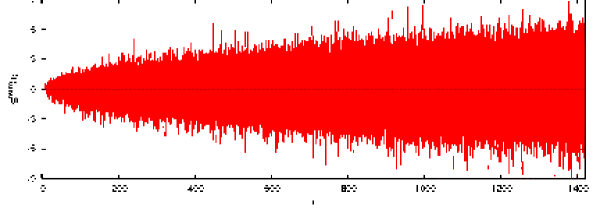
Figure 1. The fluctuations $S^{\text{num}}(t)$ for $\operatorname{SL}(2,\mathbb{Z})$.

From the graph of $\langle S^{\text{num}}(t)\rangle:=\frac{1}{t}\int_{0}^{t}S^{\text{num}}(\tau)d\tau$, we can read off whether all eigenvalues have been found. If all eigenvalues are found, $\langle S^{\text{num}}(t)\rangle$ equals $\langle S(t)\rangle$ and tends to zero in the limit of large $t$. As soon as a solution gets overseen near $\lambda=r^{2}+1/4$ with $r\geq 0$, $\langle S^{\text{num}}(t)\rangle$ deviates significantly from $\langle S(t)\rangle$ for $t>r$, $\langle S^{\text{num}}(t)\rangle\leq\langle S(t)\rangle+\frac{1}{t}\int_{r}^{t}(-1)d\tau$. This is visualised in figure 2, where we have intentionally removed the eigenvalue $\lambda_{135916}=1/4+1300.0191255^{2}$. From figure 2, we can read off that at least one eigenvalue is missing and that the first eigenvalue which is missing is somewhere near $\lambda=1/4+1300^{2}$.

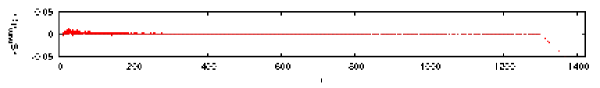
Figure 2. Mean $\langle S^{\text{num}}(t)\rangle$, with the eigenvalue $\lambda_{135916}=1/4+1300.0191255^{2}$ removed.

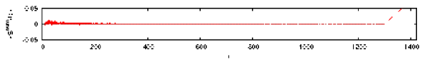
Figure 3. Mean $\langle S^{\text{num}}(t)\rangle$, with the fake “eigenvalue” $\lambda_{\text{fake}}=1/4+1300^{2}$ inserted.

On the other hand, if we are in doubt whether a given list of eigenvalues is consecutive, we can intentionally insert a fake “eigenvalue” near the end of the list. For instance, if we intentionally insert a fake “eigenvalue” $\lambda_{\text{fake}}=1/4+1300^{2}$ to the list of consecutive eigenvalues, the graph of $\langle S^{\text{num}}(t)\rangle$ will clearly show that there is one eigenvalue too much near $\lambda=1/4+1300^{2}$, see figure 3.

If we know Turing bounds for $\langle S(t)\rangle$, the comparison of $\langle S^{\text{num}}(t)\rangle$ against these bounds becomes conclusive. For the modular group, Turing bounds have been derived explicitly [6].

Theorem 15 (Turing bounds for the modular group [6]).

Consider the modular group $\Gamma=\operatorname{SL}(2,\mathbb{Z})$, and define $E(t)=\big{(}1+6.59125/\log t\big{)}\big{(}\pi/(12\log t)\big{)}^{2}$. Then for $t>1$, we have the lower and upper Turing bounds

$$E_{\text{lower}}(t):=-2E(t)<\langle S(t)\rangle<E(t)=:E_{\text{upper}}(t).$$

The proof is given in [6].

Theorem 16 (Turing’s method [33]).

If we add a fake “eigenvalue”, $\lambda_{\text{fake}}$, near the end of a list of eigenvalues, and if $\langle S^{\text{num}}(t)\rangle$ then exceeds the upper Turing bound, the list of eigenvalues is consecutive in the interval $1/4\leq\lambda\leq\lambda_{\text{fake}}$.

The importance of this theorem is highlighted in [4, 15]. For the proof, see [33].

Theorem 17.

Let a list of eigenvalues be given for which we compute $\langle S^{\text{num}}(t)\rangle$. Let lower and upper Turing bounds be given such that $-1/2<E_{\text{lower}}(t)<\langle S(t)\rangle<E_{\text{upper}}(t)<1/2$ $\forall t\geq t_{0}$, where $t_{0}>0$. Let

$$T:=\min\{\tau\geq t_{0}\ |\ \langle S^{\text{num}}(\tau)\rangle\leq E_{\text{lower}}(\tau)\}$$

and

$$t:=T\max\big{(}0,\langle S^{\text{num}}(T)\rangle-E_{\text{upper}}(T)+1\big{)}.$$

Then, we have: The list of eigenvalues is consecutive for $1/4\leq\lambda<t^{2}+1/4$, but there is an eigenvalue missing in $t^{2}+1/4\leq\lambda\leq T^{2}+1/4$.

Proof.

Since there are countably many eigenvalues, the given finite list cannot be complete, $\langle S^{\text{num}}(t)\rangle\overset{t\to\infty}{\longrightarrow}\mathcal{N}^{\text{num}}(t)-\mathcal{N}(t)\leq-1<E_{\text{lower}}(t)$. $T$ exists and we have $\langle S^{\text{num}}(T)\rangle\leq E_{\text{lower}}(T)<\langle S(T)\rangle$, which implies that the list of eigenvalues is not consecutive for $1/4\leq\lambda\leq T^{2}+1/4$.

If $\lambda=r^{2}+1/4$ is the first missed eigenvalue, we have $\langle S^{\text{num}}(T)\rangle\leq\langle S(T)\rangle+\frac{1}{T}\int_{r}^{T}(-1)d\tau<E_{\text{upper}}(T)+\frac{r-T}{T}$. Hence, $\langle S^{\text{num}}(T)\rangle\geq E_{\text{upper}}(T)+\frac{t-T}{T}$ implies $t<r$ and that all eigenvalues have been found for $1/4\leq\lambda<t^{2}+1/4$ if $t\geq 0$. ∎

Algorithm 18 (The control algorithm).

Let $\Lambda$ be a list of numerically found Maass cusp forms. Typically, $\Lambda$ is empty in the beginning.

1. Let all parameters take reasonable values.

2. Determine $t$ and $T$ according to Theorem 17.

3. Let $t^{2}+1/4=\tilde{\lambda}_{1}<\tilde{\lambda}_{2}<\ldots<\tilde{\lambda}_{\nu}=T^{2}+1/4$ be trial values, and search for eigenvalues in the neighbourhood of each trial value.

4. Use Algorithm 8 to compute the corresponding Maass cusp forms.

5. For each found Maass form, compare whether it is already in the list $\Lambda$. If not, add it to the list.

6. Let $t_{\text{old}}:=t$ and $T_{\text{old}}:=T$.

7. Determine $t$ and $T$ according to Theorem 17.

8. If $t$ is equal to $t_{\text{old}}$ and $T$ is equal to $T_{\text{old}}$, then increase $\nu$ and change all parameters to somewhat different reasonable values. Otherwise, decrease $\nu$ slightly in order to speed up the numerics.

9. Continue with 3

Theoretically, Algorithm 18 runs forever and finds an ever increasing list of consecutive Maass cusp forms.

For groups other than $\operatorname{SL}(2,\mathbb{Z})$, Turing bounds have not been derived, yet. It is possible to replace Turing bounds by heuristic bounds which follow from intentionally removing and inserting eigenvalues near the end of an almost consecutive list of eigenvalues, as was demonstrated in figures 2 and 3. However, this requires user interaction and slows down the algorithm. Results for certain moonshine groups are published in [17].

7. Fluctuations in the Weyl remainder

Here, we present results for the modular group $\Gamma=\operatorname{SL}(2,\mathbb{Z})$. It is worth while to desymmetrise the Maass cusp forms, as this speeds up their computation. On the modular surface $X=\Gamma\backslash\mathcal{H}$, Maass cusp forms fall into even, $f(-x+iy)=f(x+iy)$, and odd, $f(-x+iy)=-f(x+iy)$, eigenfunctions. Letting Algorithm 18 run for some days, we have found $80\,443$ consecutive even Maass cusp forms with $1/4\leq\lambda<1421.98^{2}+1/4$, but missed $1$ out of $81\,673$ with $1/4\leq\lambda<1432.64^{2}+1/4$ by the time when we interrupted the algorithm. For the odd symmetry, the algorithm was faster. In the same time, we have found $164\,232$ consecutive odd Maass cusp forms with $1/4\leq\lambda<2000^{2}+1/4$. The amount of data allows us to investigate the asymptotic and statistic properties of the fluctuations in the Weyl remainder $S(t)$, numerically.

From Rudnick [25] we know that the number of eigenvalues obeys a central limit theorem. In particular, he considers smoothed windows of length $1/L$ centered at points $t$, and examins the number $N_{L}(t)$ of $r_{j}$ that lie within each such window. In the limit $L\to\infty$ and $T\to\infty$ but $L=o(\log T)$, the distribution of $N_{L}(t)$ as $t$ varies through $[T,2T]$ approaches a Gaussian,

$$\lim_{T\to\infty}\frac{1}{T}\operatorname{meas}\{t\in[T,2T]:\frac{N_{L}(t)-\overline{N_{L}}(t)}{\sigma_{L}}<x\}=\int_{-\infty}^{x}e^{-u^{2}/2}\frac{du}{\sqrt{2\pi}}.$$

We ask whether the fluctuations in the Weyl remainder (without smoothing) also obey a central limit theorem.

In view of figure 1, we note that the magnitude of the remainder fluctuations grows in $t$, and we may better consider a scaled version of the Weyl remainder. From Li and Sarnak [19] we know a lower bound on the asymptotic growth rate of the remainder fluctuations,

$$S(t)=\Omega\Big{(}\frac{t^{1/2}}{\log t}\exp\big{(}\tfrac{1}{2}(\log\log t)^{5/17}\big{)}\Big{)}.$$

Figure 4 shows how close this lower bound is to the true asymptotic growth rate. Concerning an upper bound, nothing better than $S(t)=O(t/\log t)$ is known analytically.

Conjecture 19.

On the modular surface $X=\operatorname{SL}(2,\mathbb{Z})\backslash\mathcal{H}$, the asymptotic growth rate of the remainder fluctuations is bounded from above by

$$S(t)=o(\sqrt{t}).$$

Numerical evidence for the conjecture is displayed in figure 5, where the magnitude of fluctuations of $\frac{1}{\sqrt{t}}|S(t)|$ slightly decreases with $t$.

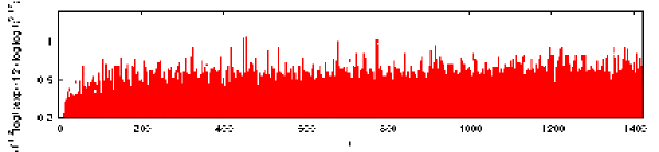
Figure 4. A graph of $\frac{\log t}{\sqrt{t}}\exp\big{(}-\tfrac{1}{2}(\log\log t)^{5/17}\big{)}|S(t)|$ whose magnitude of fluctuations slightly increases with $t$. This eventually lets the $\limsup$ of the graph diverge in the limit $t\to\infty$. The graph also shows how close the lower bound of Li and Sarnak comes to the true asymptotic growth rate.

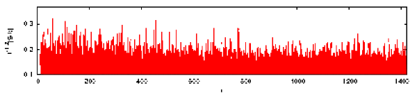
Figure 5. A graph of $\frac{1}{\sqrt{t}}|S(t)|$ whose magnitude of fluctuations slightly decreases with $t$. This eventually lets the graph vanish in the limit $t\to\infty$.

Conjecture 20.

Consider the fluctuations in the Weyl remainder $S(t)$ on the modular surface $X=\operatorname{SL}(2,\mathbb{Z})\backslash\mathcal{H}$. If scaled by $\frac{\log\log t}{\sqrt{t}}$, the fluctuations obey a central limit theorem. For any ${\mathcal{L}}>0$, we have

$$\lim_{T\to\infty}\frac{1}{\mathcal{L}}\operatorname{meas}\{t\in[T,T+{\mathcal{L}}]:\frac{\log\log t}{\sqrt{t}}\frac{S(t)}{\sigma}<x\}=\int_{-\infty}^{x}e^{-u^{2}/2}\frac{du}{\sqrt{2\pi}},$$

with $\sigma\approx 0.140$.

A histogram of the scaled distribution is shown in figure 6.

Figure 6. Distribution of $\frac{\log\log t}{\sqrt{t}}\frac{S(t)}{\sigma}$ (solid curve) as $t$ varies through $[0,1421.98]$, in comparison with the standard Gaussian (dashed curve).

The scale factor $\frac{\log\log t}{\sqrt{t}}$ results from numerical considerations. Namely, if we examine $S(t)$ in the interval $[a,b]$, the mean and the variance of the scaled fluctuations,

$$\mu_{[a,b]}=\frac{1}{b-a}\int_{a}^{b}\frac{\log\log t}{\sqrt{t}}S(t)dt,$$

$$\sigma_{[a,b]}^{2}=\frac{1}{b-a}\int_{a}^{b}\Big{(}\frac{\log\log t}{\sqrt{t}}S(t)-\mu_{[a,b]}\Big{)}^{2}dt,$$

are numerically independent of $t$. Quantitative results for $\mu_{[t-100,t+100]}$ and $\sigma_{[t-100,t+100]}$ in dependence of $t$ are shown in figure 7. We find that the mean vanishes $\mu\approx 0$ and that the standard deviation is constant $\sigma\approx 0.140$.

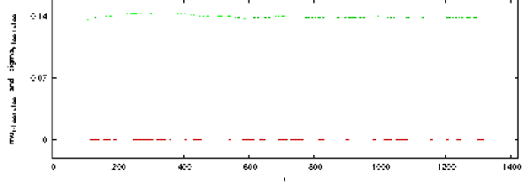
Figure 7. Plots of the mean $\mu_{[t-100,t+100]}$ and the standard deviation $\sigma_{[t-100,t+100]}$ in dependence of $t$.

By analogy with the law of the iterated logarithm, one might expect the correct scalings for the distribution and extreme values to differ by a factor of $\sqrt{\log\log t}$. However, for the $S(t)$ of Riemann zeta, it’s thought [9] that they differ by about $\sqrt{\log t}$, which is quite a bit larger. We expect that the difference between the $S(t)$ of Maass form eigenvalues and that of Riemann zeros comes from the level statistics. The eigenvalues of the Laplacian on arithmetic surfaces are expected to be Poisson distributed [2, 3], whereas the Riemann zeros are expected to lie on the critical line and show a distribution in resemblance to the eigenvalues of random matrices of the Gaussian unitary ensemble [22, 26].

We believe that the iterated logarithm heuristic is closer to the truth. If the Weyl remainder would result from a Wiener process, it would strictly follow the law of the iterated logarithm and we would have

$$\limsup_{t\to\infty}\Big{(}\frac{\log\log t}{2t}\Big{)}^{1/2}|S(t)|=\sigma.$$

We have checked this numerically and find that the predicted scaling of extreme values agrees with our numerical data. The scaling also agrees with the upper bound of Conjecture 19. However, the numerical values of the extrema are larger than predicted by a factor of $2.5$, i.e. we find

$$\limsup_{t\to\infty}\Big{(}\frac{\log\log t}{2t}\Big{)}^{1/2}|S(t)|\approx 2.5\sigma,$$

which indicates that the fluctuations in the Weyl remainder do not exactly follow the law of the iterated lagarithm.

References

- [1] R. Aurich, S. Lustig, F. Steiner, and H. Then, Hyperbolic universes with a horned topology and the cosmic microwave background anisotropy, Class. Quantum. Grav. 21 (2004), 4901–4925.
- [2] E. B. Bogomolny, B. Georgeot, M.-J. Giannoni, and C. Schmit, Chaotic billiards generated by arithmetic groups, Phys. Rev. Lett. 69 (1992), 1477–1480.
- [3] J. Bolte, G. Steil, and F. Steiner. Arithmetical chaos and violation of universality in energy level statistics. Phys. Rev. Lett. 69 (1992), 2188–2191.
- [4] A. R. Booker, Turing and the Riemann hypothesis, AMS Notices 53 (2006), 1208–1211.
- [5] A. R. Booker et al., Real quadratic class number certification, (in preparation).
- [6] A. R. Booker and A. Strömbergsson, Theoretical and practical aspects of Maass form computation, (in preparation).
- [7] A. R. Booker, A. Strömbergsson, and H. Then, Bounds and algorithms for the K-Bessel function of imaginary order, to appear in the LMS J. Comp. Math..
- [8] A. R. Booker, A. Strömbergsson, A. Venkatesh, Effective computation of Maass cusp forms, IMRN 2006, Article ID 71281, 34 pages.
- [9] D. W. Farmer, S. M. Gonek, and C. P. Hughes, The maximum size of L-functions, J. Reine Angew. Math. 609 (2007), 215–236.
- [10] L. Flaminio and G. Forni, Invariant distributions and time averages for horocycle flows, Duke Math. J. 119 (2003), 465–526.
- [11] D. A. Hejhal, The Selberg Trace Formula for PSL(2,R), Lecture Notes in Mathematics 548 (1973) and 1001 (1983), Springer.
- [12] D. A. Hejhal, On value distribution properties of automorphic functions along closed horocycles. In XVIth Rolf Nevanlinna Colloquium (Joensuu, Finnland, 1995), de Gruyter, Berlin, 1996, 39–52.
- [13] D. A. Hejhal. On eigenfunctions of the Laplacian for Hecke triangle groups. In D. A. Hejhal, J. Friedman, M. C. Gutzwiller, and A. M. Odlyzko, editors, Emerging Applications of Number Theory, IMA Series No. 109, pp. 291–315. Springer, 1999.
- [14] D. A. Hejhal, On the uniform equidistribution of long closed horocycles. Loo-Keng Hua: a great mathematician of the twentieth century, Asian J. Math. 4 (2000), 839–853.
- [15] D. A. Hejhal and A. M. Odlyzko, Alan Turing and the Riemann zeta function. In S. B. Cooper and J. van Leeuwen, editors, Alan Turing – His Work and Impact, Elsevier, to appear.
- [16] D. A. Hejhal and B. Rackner, On the topography of Maass waveforms for PSL(2,Z), Experiment. Math. 1 (1992), 275–305.
- [17] J. Jorgenson, L. Smajlović, and H. Then, On distribution of eigenvalues of Maass forms on certain moonshine groups, (submitted).
- [18] S. Katok, Fuchsian Groups, Chicago Lectures in Mathematics, University of Chicago Press, 1992.
- [19] X. Li and P. Sarnak, Number variance for SL(2,Z)H, http://web.math.princeton.edu/sarnak/SarnakNumberPaper04.pdf
- [20] E. Lindenstrauss, Invariant measures and arithmetic quantum unique ergodicity, Ann. of Math. (2) 163 (2006), 165–219.
- [21] H. Maass, Über eine neue Art von nichtanalytischen automorphen Funktionen und die Bestimmung Dirichletscher Reihen durch Funktionalgleichungen, Math. Annalen 121 (1949), 141–183.
- [22] L. Montgomery, The pair correlation of zeros of the zeta function, Analytic Number Theory (Proc. Sympos. Pure Math., Vol. XXIV, St. Louis Univ., St. Louis, Mo., 1972), Proc. Sympos. Pure Math., vol. 24, Amer. Math. Soc., Providence, 1973, 181–193.
- [23] W. Roelcke, Über die Wellengleichung bei Grenzkreisgruppen erster Art, Sitzungsberichte Heidelberger Akad. Wiss. Math.-nat. Kl. 1953/55, Abh. 4 (1956), 159–267.
- [24] W. Roelcke, Das Eigenwertproblem der automorphen Formen in der hyperbolischen Ebene, I and II, Math. Ann. 167 (1966), 292–337, and 168 (1967), 261–324.
- [25] Z. Rudnick, A central limit theorem for the spectrum of the modular domain, Ann. Henri Poincaré 6 (2005), 863–883.
- [26] Z. Rudnick and P. Sarnak, Zeros of principal L-functions and random matrix theory, Duke Math. J. 81 (1996), 269–322.
- [27] A. Ruhe, Algorithms for the nonlinear eigenvalue problem, SIAM J. Num. Anal. 10 (1973), 674–689.
- [28] P. Sarnak, Asymptotic behavior of periodic orbits of the horocycle flow and Eisenstein series, Comm. Pure Appl. Math. 34 (1981), 719–739.
- [29] P. Sarnak, Problems of the Millenium: The Riemann Hypothesis (2004), Clay Mathematics Institute http://www.claymath.org/millennium/Riemann_Hypothesis/
- [30] A. Selberg, Harmonic analysis and discontinuous groups in weakly symmetric Riemannian spaces with applications to Dirichlet series, J. Indian Math. Soc. (N.S.) 20 (1956), 47–87.
- [31] A. Strömbergsson, A pullback algorithm for general (cofinite) Fuchsian groups, (2000), http://www2.math.uu.se/~astrombe/papers/pullback.ps
- [32] A. Strömbergsson, On the uniform equidistribution of long closed horocycles, Duke Math. J. 123 (2004), 507–547.
- [33] A. M. Turing, Some calculations of the Riemann zeta-function, Proc. London Math. Soc. 3 (1953), 99–117.
- [34] D. Zagier, Eisenstein series and the Riemann zeta function. In Automorphic Forms Representation Theory and Arithmetic (Bombay, 1979), Tata Inst. Fund. Res. Studies in Math. 10, Tata Inst. Fundamental Res., Bombay, 1981, 275–301.