Interdependency and hierarchy of exact and approximate epidemic models on networks

Abstract

Over the years numerous models of $SIS$ (susceptible $\rightarrow$ infected $\rightarrow$ susceptible) disease dynamics unfolding on networks have been proposed. Here, we discuss the links between many of these models and how they can be viewed as more general motif-based models. We illustrate how the different models can be derived from one another and, where this is not possible, discuss extensions to established models that enables this derivation. We also derive a general result for the exact differential equations for the expected number of an arbitrary motif directly from the Kolmogorov/master equations and conclude with a comparison of the performance of the different closed systems of equations on networks of varying structure.

1 Introduction

Modeling the spread of infectious diseases requires an understanding of not only disease characteristics but also an understanding of the community (be it a hospital, school, town, etc) in which it pervades. An important consideration in modelling the spread of diseases is thus the contact structure on which disease transmission happens. Whereas traditional approaches ([2, 6]) assume little or no topological structure, recent work ([15, 16, 17]) has tried to incorportate the underlying linkages between entities in the population and study how these links facilitate the spread of the disease. For a continuous-time stochastic disease transmission model on an arbitrary network it is possible ([13]), to write down the relevant Kolmogorov/master equations and thus model it as a continuous time Markov chain that fully describes the movement between all possible system states. Unfortunately the complexity of the model comes from the size of the state space and the number of equations scales exponentially as $a^{N}$, where $a$ is the number of different states a node can be in and $N$ is the network size. One widely used resolution to this complexity is to create individual-based simulation models and investigate the system behaviour directly. Even though increasing computational power makes simulations an increasingly attractive proposition they lack analytic tractability. Whilst this is not always a hindrance, when the system displays a rich range of behaviour (e.g. oscillations, bistability) it may not be feasable to obtain a global overview of the effects of different parameter values and thus the more analytic approach is needed. For this reason, low-dimensional systems of differential equations ([15, 7, 17]) are sought provided that these can approximate the exact solution. By reducing the problem to a smaller system of equations it is easier to study the bifurcation structure of the model and gain a greater understanding of the full spectrum of behaviour. The challenge is then finding the set of equations that best approximate the solution of the Kolmogorov equations.

Given that here we focus on epidemic models, usually such models are formulated in terms of the expected values of the number of infected and/or susceptible individuals or some other motif in the network such as the expected number of infected and/or susceptible individuals of different degrees (the number of connections a node has). Such models range from classic meanfield [1] to pairwise [15], heterogenous pairwise [7], effective degree [17, 18] and individual-level models [22] to name a few. Whilst these models seem to use different approaches their derivation is based on the same conceptual framework, namely they begin by choosing a base-motif (e.g. a node, a link and the two nodes it connects, a node and all its links). These base-motifs are then used to formulate equations for the different possible states that they can achieve (e.g. for the expected number of motifs in different states or the probability that a specified motif in the network is in a certain state). These equations generally involve not only the base-motif itself, but larger or extended motifs of which they are usually part of. These larger motifs in turn depend on more complex motifs and a closure is needed in order to obtain a self-contained system of equations of reasonable size. Importantly the base-motif determines not only the complexity of the model (the larger the motif the greater the number of states it can be in) but also how much of the network topology can be captured. Interestingly differential equations for smaller motifs that are part of the base-motif should, in theory, be recoverable from the original differential equation. To this end the main focus of the paper is the consideration of various simple models of disease dynamics and the relations between them. We also consider which models are derivable directly (subject to a suitable closure) from the Kolmogorov/master equations and can thus be referred to as exact.

We begin in section 2 with an introduction of some of the more common approaches to modelling disease dynamics on networks, considering meanfield ([1]), pairwise ([15]), heterogeneous pairwise ([7]) and the effective degree ([17]) model formulations. In section 3 we formulate an exact version of the effective degree model and then illustrate how the pairwise model can then be recovered from this new set of equations. We are, however, unable to recover the heterogenous pairwise model from the exact effective degree and this motivates, in section 4, an extension of this which incorporates further network topology into the ODEs. From this extension we then show how it is then possible to recover the heterogeneous pairwise equations. Once the links between the models have been established, in section 5 we show how the unclosed version of the models can be derived directly from the Kolmogorov equations. This is done by proving that as long as the heuristic equations for any motif are written following a certain set of rules they will always be exact. We conclude, in section 5 with a brief comparison of the models and discuss under what circumstances they perform best, in the sense of being close to simulation results.

2 Models of disease dynamics

In this paper we focus on susceptible $\rightarrow$ infected $\rightarrow$ susceptible ($SIS$) disease dynamics on networks but note that all of the following models can be adapted for other disease (e.g. $SIR$ and/or contact tracing) or non-disease (e.g. evolutionary [10]) dynamics. With this in mind we use $\tau$ as the per-link transmission rate between susceptible and infected nodes and $\gamma$ as the recovery rate of an infected individual. Both infection and recovery are modelled as independent poisson processes. As a starting point we give a short summary of ODE-based models that are either exact or an approximation of the true dynamics resulting from the full system based on the Kolmogorov/master equations, where these are solvable, or based on simulation.

2.1 Pairwise and the resulting simple compartmental model

In order to focus on the underlying network of contacts, we introduce the pairwise model first ([15, 21]). The main idea of this model is to develop the hierarchical dependence of lower order moments (e.g. expected number of susceptible $[S]$ and infected $[I]$ nodes) on higher ones (e.g. expected number of pairs with one susceptible and one infected node, $[SI]$) and to derive appropriate models that correctly account for these. As already suggested, the expected number of pairs will depend on larger motifs, in this case these being the expected number of triples denoted by $[ABC]$, where $A,B,C\in\{S,I\}$ and $B$ is connected to $A$ and $C$. Using this notation the equations governing the evolution of the disease dynamics at the level of singles and pairs are given by

$$\frac{d}{dt}\left[I\right] =-\gamma\left[I\right]+\tau\left[SI\right],$$ (1)

$$\frac{d}{dt}\left[SS\right] =-2\tau[ISS]+2\gamma[IS],$$ (2)

$$\frac{d}{dt}\left[SI\right] =\tau\left([ISS]-[ISI]-[IS]\right)+\gamma\left([II]-[IS]\right),$$ (3)

$$\frac{d}{dt}\left[II\right] =2\tau\left([ISI]+[SI]\right)-2\gamma[II].$$ (4)

Here we consider ordered pairs and triples, meaning they are counted in both directions. For pairs (with similar remarks for triples) this means $[IS]=[SI]$ and links of type $S-S$ and $I-I$ have a double contribution to the $[SS]$ and $[II]$ counts. Importantly we note that these equations are unclosed as no equations are given for the evolution of the triples. The standard closure (in the absence of clustering) makes the assumption that the status of pairs are statistically independent of one another and then

$$\left[ABC\right]\approx [AB](n-1)\frac{[BC]}{n[B]},$$

where $n$ is the average degree of the network. When we use this closure we say we have closed “at the level of triples” . In order to derive the classic mean-field model a closure at the level of paris can be applied, namely, $[SI]$ can be approximated as

$$[SI]\approx n[S]\frac{[I]}{N}$$

and upon using Eq. (1), the classic mean-field model can be recovered

$$\frac{d}{dt}\left[I\right] =-\gamma\left[I\right]+\tau n\left[S\right]\frac{\left[I\right]}{N},$$ (5)

where the widely used transmission rate from the compartmental model,[1], is $\beta=\tau n$.

It is also important to note that the unclosed equations above (Eqs. (1-4)) can be derived directly from the state-based Kolmogorov equations and for this reason we refer to these equations as exact. Whilst a proof for the exactness of these equations was given in [23], in section 5 we provide a more general proof that allows us to write down exact equations for, not just pairs, but any motif structure. We also note that an alternative approach was used by Sharkey in [22], to prove that the standard pairwise equations were exact for models with susceptible $\rightarrow$ infected $\rightarrow$ recovered ($SIR$) disease dynamics.

2.2 Heterogeneous pairwise model

Whilst the pairwise equations perform well in capturing disease dynamics on networks that are well described by their average degree, the closure assumption fails when greater heterogeneity is introduced. More precisely, whilst the pairwise equations above are exact for an arbitrary network before a closure, these do not guarantee that with the current choice of singles and pairs (i.e. $[S]$ could be further divided to account for heterogeneity in degree) a valid closure could be found for any network. Indeed, to account for greater heterogeneity Eames et al. [7] further developed the pairwise model by taking into account not just the state of nodes and pairs but also the degrees of the nodes. By using $[A^{n}]$ to represent expected number of nodes of type $A$ with degree $n$ and with similar notation for pairs and triples, they were able to formulate the following set of unclosed equations

$$\frac{d}{dt}\left[S^{n}\right] =\gamma\left[I^{n}\right]-\tau\sum_{q}{\left[S^{n}I^{q}\right]},$$ (6)

$$\frac{d}{dt}\left[I^{n}\right] =-\gamma\left[I^{n}\right]+\tau\sum_{q}{\left[S^{n}I^{q}\right]},$$ (7)

$$\frac{d}{dt}\left[S^{n}S^{m}\right] =-\tau\sum_{q}{\left(\left[S^{n}S^{m}I^{q}\right]+\left[I^{q}S^{n}S^{m}\right]\right)}+\gamma\left(\left[S^{n}I^{m}\right]+\left[I^{n}S^{m}\right]\right),$$ (8)

$$\frac{d}{dt}\left[S^{n}I^{m}\right] =\tau\sum_{q}{\left(\left[S^{n}S^{m}I^{q}\right]-\left[I^{q}S^{n}I^{m}\right]\right)}-\tau\left[S^{n}I^{m}\right]-\gamma\left[S^{n}I^{m}\right]+\gamma\left[I^{n}I^{m}\right],$$ (9)

$$\frac{d}{dt}\left[I^{n}I^{m}\right] =\tau\sum_{q}{\left(\left[I^{n}S^{m}I^{q}\right]+\left[I^{q}S^{n}I^{m}\right]\right)}+\tau\left[I^{n}S^{m}\right]+\tau\left[S^{n}I^{m}\right]-2\gamma\left[I^{n}I^{m}\right].$$ (10)

Again assuming the statistical independence of pairs and absence of clustering, Eames et. al, [7], suggest the following approximations of triples

$$\left[B^{n}C^{m}D^{p}\right]\approx [B^{n}C^{m}](m-1)\frac{[C^{m}D^{p}]}{m[C^{m}]}.$$

2.3 The effective degree model

In [17], Lindquist et  al. introduced the effective degree model for $SIS$ (and also $SIR$) dynamics on a network (an equivalent model formulation was also proposed by Marceau et al. [18]). In this model they consider not only the state of a node ($S$ or $I$), but also the number of the immediate neighbours in the various potential states. This is done by writing the following set of equations for all the possible star-like motifs in the network where $S_{s,i}$ ($I_{s,i}$) represents the expected number of susceptible (infected) nodes with $s$ susceptible and $i$ infected neighbours,

$$\dot{S}_{s,i}= -\tau iS_{s,i}+\gamma I_{s,i}+\gamma[(i+1)S_{s-1,i+1}-iS_{s,i}]$$

$$+\tau\frac{\sum_{k=1}^{M}\sum_{j+l=k}jlS_{j,l}}{\sum_{k=1}^{M}\sum_{j+l=k}jS_{j,l}}[(s+1)S_{s+1,i-1}-sS_{s,i}],$$ (11)

$$\dot{I}_{s,i}= \tau iS_{s,i}-\gamma I_{s,i}+\gamma[(i+1)I_{s-1,i+1}-iI_{s,i}]$$

$$+\tau\frac{\sum_{k=1}^{M}\sum_{j+l=k}l^{2}S_{j,l}}{\sum_{k=1}^{M}\sum_{j+l=k}jI_{j,l}}[(s+1)I_{s+1,i-1}-sI_{s,i}],$$ (12)

with $1\leq s+i\leq M$, where $M$ is the maximum degree and the equations are suitably adjusted on the boundaries. It is important to note that this model is not exact as a closure has been already applied. Namely the infection of a node’s susceptible neighbours is based on a population-level approximation. To illustrate this more precisely we borrow the notation of the pairwise model and make two observations

$$\frac{\sum_{k=1}^{M}\sum_{j+l=k}jlS_{j,l}}{\sum_{k=1}^{M}\sum_{j+l=k}jS_{j,l}} =\frac{[ISS]}{[SS]},$$

$$\frac{\sum_{k=1}^{M}\sum_{j+l=k}l^{2}S_{j,l}}{\sum_{k=1}^{M}\sum_{j+l=k}jI_{j,l}} =\frac{\sum_{k=1}^{M}\sum_{j+l=k}l(l-1)S_{j,l}+lS_{j,l}}{\sum_{k=1}^{M}\sum_{j+l=k}jI_{j,l}}=\frac{[ISI]+[SI]}{[SI]}=\frac{[ISI]}{[SI]}+1.$$

These means that the infection pressure on the susceptible neighbours of the central node is equal to the population level average taken from all the possible star-like configurations rather then from the extended star structures that would account exactly for these infections.

3 Recovering the pairwise model from the effective degree

Whilst the pairwise and effective degree models seem different they are based on a similar approach. Both models work on approximating the evolution of different motifs in the network; individuals and links in the pairwise model and star-like structures in the effective degree. For both models, but more clearly for the pairwise, the models begin with a starting or base motif (e.g. nodes) for which an evolution equation is required. This will of course depend on an extended motif, typically the base motif extended by the addition of an extra node (e.g. pairs). This dependency on higher order motifs continues, for example, with pairs depending on triples, and then triples depending on quadruplets (four nodes connected by a line, i.e. $A-B-C-D$, or a star with a centre and three spokes, i.e. $A-\overbracket{B-C\quad D}$). Hence, the models only differ in the choice of the base motif and then potentially in the way in which the systems are closed to curtail the dependency on higher order motifs. Since, here we are mainly interested in exact models, that is before a closure is applied, we begin by conjecturing an exact version of the effective degree model and show how starting from this the exact pairwise model can be derived.

3.1 Exact effective degree

Based on the ideas presented above, we extend the star-like base motif to reveal the dependence on higher order motifs and conjecture that this unclosed version of the effective degree model is exact. We begin by introducing a variable to count the expected number of infecteds connected to a node’s susceptible neighbours. This is done by introducing two new terms, $[ISS_{s^{\prime},i^{\prime}}]$ and $[ISI_{s^{\prime},i^{\prime}}]$. For the term $[ISI_{s^{\prime},i^{\prime}}]$ (and similarly for $[ISS_{s^{\prime},i^{\prime}}]$) the $S$ in the middle is actually used to represent the susceptible neighbours of the central $I$ from the motif with composition $I_{s^{\prime}i^{\prime}}$ (i.e. the $I$ node with neighbourhood $(s^{\prime},i^{\prime})$ is the centre of the star, while $S$ is a susceptible spoke). The $I$ (on the left-hand side), in turn, represents the infective neighbours of these susceptibles’ and within this count, in the case of $[ISI_{s^{\prime},i^{\prime}}]$, we also include the originating central $I$. The exact effective degree model can then be written as

$$\dot{S}_{s,i}= -\tau iS_{s,i}+\gamma I_{s,i}+\gamma[(i+1)S_{s-1,i+1}-iS_{s,i}]$$

$$+\tau\left[ISS_{s+1,i-1}\right]-\tau\left[ISS_{s,i}\right],$$ (13)

$$\dot{I}_{s,i}= \tau iS_{s,i}-\gamma I_{s,i}+\gamma[(i+1)I_{s-1,i+1}-iI_{s,i}]$$

$$+\tau\left[ISI_{s+1,i-1}\right]-\tau\left[ISI_{s,i}\right].$$ (14)

Fig. 1 shows the possible transitions captured by this model.

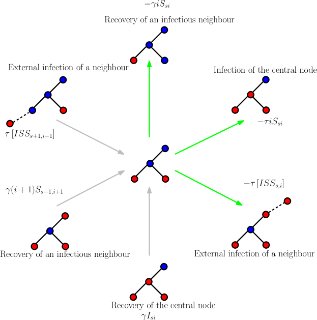
Figure 1: Illustration of the transitions into and out of the $S_{2,1}$ class. Susceptible nodes are given in blue and infective nodes in red. Transitions into and out of the class are shown in grey and green, respectively. The corresponding terms of the general equation are also given. In Appendix $1$ a similar illustration is given for a configuration with a centrally infectious node.

3.2 Recovering the pairwise equations

The star-like composition of the effective degree model allows us to recover the pairwise equations via careful summations. The full derivation of the pairwise model is given in Appendix $2$, whilst here we only illustrate the derivation of the individuals (trivial but given for completeness) and the [$II$] pairs,

$$\frac{d}{dt}\left[S\right] =\sum_{s,i}\dot{S}_{s,i}=\gamma\left[I\right]-\tau\left[SI\right],$$

$$\frac{d}{dt}\left[I\right] =\sum_{s,i}\dot{I}_{s,i}=-\gamma\left[I\right]+\tau\left[SI\right],$$

where most terms from the original effective degree equations cancel and we have used that $\sum_{s,i}iS_{s,i}=[SI]$ and $\sum_{s,i}I_{s,i}=[I]$. For $[II]$ the following equality holds

$$\frac{d}{dt}\left[II\right]= \sum_{s,i}i\dot{I}_{s,i}$$

$$= \tau\sum{i^{2}S_{s,i}}-\gamma\sum{iI_{s,i}}+\gamma\sum{i(i+1)I_{s-1,i+1}}-\gamma\sum{i^{2}I_{s,i}}$$

$$+\tau\sum{i[ISI_{s+1,i-1}]}-\tau\sum{i[ISI_{s,i}]}$$

$$= \tau\sum{i(i-1)S_{s,i}}+\tau\sum{iS_{s,i}}-\gamma[II]$$

$$+\gamma[III]-\gamma\sum{i(i-1)I_{s,i}}-\gamma\sum{iI_{s,i}}$$

$$+\tau\sum{(i-1)[ISI_{s+1,i-1}]}+\tau\sum{[ISI_{s+1,i-1}]}-\tau\sum{i[ISI_{s,i}]}$$

$$= \tau[ISI]+\tau[IS]-\gamma[II]+\gamma[III]-\gamma[III]-\gamma[II]+\tau[ISI]+\tau[IS]$$

$$= 2\tau\left([ISI]+[IS]\right)-2\gamma[II],$$

where we have used that $\sum_{s,i}iI_{si}=[II]$, $\sum_{s,i}{(i-1)[ISI_{s+1,i-1}]}=\sum{i[ISI_{s,i}]}$ and that $\sum{[ISI_{s+1,i-1}]}=[ISI]+[SI]$. These all follow from the definition of the pairwise model and the definition of the new extended motifs from the exact effective degree model. We note that this result does indeed correspond to that of the given pairwise model.

4 Higher order models

Whilst we can recover the pairwise equations from the exact effective degree model we note that the same is not possible with the heterogeneous pairwise equations. This motivates an extension of the effective degree model where the degrees of neighbouring nodes are also taken in to account. Again we conjecture that this model can, in theory, be derived from the exact Kolmogorov equations and thus refer to it as exact.

4.1 Exact effective degree with neighbourhood composition

We extend the exact effective degree model to include the number of neighbours of the central nodes’ neighbours. We begin by defining the following notation

$$s^{\prime} =(s_{1},s_{2},\ldots,s_{M}),$$

$$i^{\prime} =(i_{1},i_{2},\ldots,i_{M}),$$

$$|s^{\prime}| =s_{1}+s_{2}+\ldots+s_{M},$$

$$|i^{\prime}| =i_{1}+i_{2}+\ldots+i_{M},$$

where $s_{j}$ ($i_{j}$) represents the number of susceptible (infective) neighbours of degree $j$. We now define $S_{s^{\prime}i^{\prime}}$, ($I_{s^{\prime}i^{\prime}}$) as the number of susceptible (infective) nodes with neighbouring nodes whose own degrees are given by the entries in $s^{\prime}$ and $i^{\prime}$. We can now write the extended ODEs in the following form

$$\dot{S}_{s,^{\prime}i^{\prime}}= -\tau|i^{\prime}|S_{s,^{\prime}i^{\prime}}+\gamma I_{s^{\prime},i^{\prime}}+\gamma\sum_{k=1}^{M}{(i_{k}+1)S_{s^{\prime}_{k-},i^{\prime}_{k+}}}-\gamma|i^{\prime}|S_{s^{\prime},i^{\prime}}$$

$$+\tau\sum_{k=1}^{M}{\left[IS^{k}S_{s^{\prime}_{k+},i^{\prime}_{k-}}\right]}-\tau\left[ISS_{s^{\prime},i^{\prime}}\right],$$ (15)

$$\dot{I}_{s^{\prime},i^{\prime}}= \tau|i^{\prime}|S_{s^{\prime},i^{\prime}}-\gamma I_{s^{\prime},i^{\prime}}+\gamma\sum_{k=1}^{M}{(i_{k}+1)I_{s^{\prime}_{k-},i^{\prime}_{k+}}}-\gamma|i^{\prime}|I_{s^{\prime},i^{\prime}}$$

$$+\tau\sum_{k=1}^{M}{\left[IS^{k}I_{s^{\prime}_{k+},i^{\prime}_{k-}}\right]}-\tau\left[ISI_{s^{\prime},i^{\prime}}\right].$$ (16)

Here $s^{\prime}_{k-}=(s_{1},s_{2},\ldots,s_{k}-1,\ldots,s_{M})$ and $s^{\prime}_{k+}=(s_{1},s_{2},\ldots,s_{k}+1,\ldots,s_{M})$ with a similar definition for $i^{\prime}_{k-}$ and $i^{\prime}_{k+}$. With a small modification to the exact effective degree notation terms such as $\left[IS^{k}S_{s^{\prime}_{k+},i^{\prime}_{k-}}\right]$ are taken to represent number of infectious contacts of the susceptible neighbours of degree $k$.

4.2 Model recovery

Here we show how, from the extended effective degree model, we can recover the heterogenous pairwise model. It is also straightforward to show, and thus omitted here, that the extended effective degree leads to the simpler exact effective degree. In turn, it also follows easily that both the exact effective degree and heterogenous pairwise models reduce to the standard pairwise model. This hierarchy of recovery is illustrated in Fig. 2.

4.2.1 Recovering the heterogeneous pairwise model from the extended effective degree

As earlier we make use of careful summation to recover the model. The full derivation is provided in Appendix $3$ so here we just provide the derivation at the individual level and of the [$I^{l}I^{n}$] pairs. For singles the following identities hold,

$$\frac{d}{dt}\left[S^{n}\right] =\sum_{|s^{\prime}|+|i^{\prime}|=n}\dot{S}_{s^{\prime},i^{\prime}}=\gamma\left[I^{n}\right]-\tau\left[S^{n}I\right],$$

$$\frac{d}{dt}\left[I^{n}\right] =\sum_{|s^{\prime}|+|i^{\prime}|=n}\dot{I}_{s^{\prime},i^{\prime}}=-\gamma\left[I^{n}\right]+\tau\left[S^{n}I\right],$$

where most terms from the original effective degree cancel and we have used that

$$\sum_{|s^{\prime}|+|i^{\prime}|=n}I_{s^{\prime},i^{\prime}}=[I^{n}]\quad\text{ and }\sum_{|s^{\prime}|+|i^{\prime}|=n}|i^{\prime}|S_{s^{\prime},i^{\prime}}=[S^{n}I].$$

For the $[I^{l}I^{n}]$ pair we obtain

$$\frac{d}{dt}\left[I^{l}I^{n}\right]= \sum_{|s^{\prime}|+|i^{\prime}|=n}{i_{l}\dot{I}_{s^{\prime},i^{\prime}}}$$

$$= \tau\sum{i_{l}|i^{\prime}|S_{s^{\prime},i^{\prime}}}-\gamma\sum{i_{l}I_{s^{\prime},i^{\prime}}}+\gamma\sum{i_{l}\sum_{k=1}^{M}{(i_{k}+1)I_{s^{\prime}_{k-}i^{\prime}_{k+}}}}$$

$$-\gamma\sum{i_{l}|i^{\prime}|I_{s^{\prime},i^{\prime}}}+\tau\sum{i_{l}\sum_{k=1}^{M}{\left[IS^{k}I_{s^{\prime}_{k+},i^{\prime}_{k-}}\right]}}-\tau\sum{i_{l}\left[ISI_{s^{\prime},i^{\prime}}\right]}$$

$$= \tau\sum{i_{l}\left(|i^{\prime}|-1\right)S_{s^{\prime},i^{\prime}}}+\tau\sum{i_{l}S_{s^{\prime},i^{\prime}}}-\gamma\left[I^{l}I^{n}\right]$$

$$+\gamma\left[I^{l}I^{n}I\right]-\gamma\sum{i_{l}\left(|i^{\prime}|-1\right)I_{s^{\prime},i^{\prime}}}-\gamma\sum{i^{\prime}_{l}I_{s^{\prime},i^{\prime}}}$$

$$+\tau\sum{i_{l}\sum_{k\neq l}{\left[IS^{k}I_{s^{\prime}_{k+},i^{\prime}_{k-}}\right]}}+\tau\sum{\left(i_{l}-1\right)\left[IS^{l}I_{s^{\prime}_{l+},i^{\prime}_{l-}}\right]}$$

$$+\tau\sum{\left[IS^{l}I_{s^{\prime}_{l+},i^{\prime}_{l-}}\right]}-\tau\sum{i_{l}\left[ISI_{s^{\prime},i^{\prime}}\right]}$$

$$= \tau\left[I^{l}S^{n}I\right]+\tau\left[I^{l}S^{n}\right]-2\gamma\left[I^{l}I^{n}\right]$$

$$+\gamma\left[I^{l}I^{n}I\right]-\gamma\left[I^{l}I^{n}I\right]+\tau\left[IS^{l}I^{n}\right]+\tau\left[S^{l}I^{n}\right]$$

$$= \tau\left[I^{l}S^{n}I\right]+\tau\left[I^{l}S^{n}\right]-2\gamma\left[I^{l}I^{n}\right]+\tau\left[IS^{l}I^{n}\right]+\tau\left[S^{l}I^{n}\right]$$

$$= \tau\sum_{q}{\left(\left[I^{l}S^{n}I^{q}\right]+\left[I^{q}S^{l}I^{n}\right]\right)}+\tau\left[I^{l}S^{n}\right]+\tau\left[S^{l}I^{n}\right]-2\gamma\left[I^{l}I^{n}\right].$$

Again, we note that this result corresponds to previously given heterogenous pairwise model.

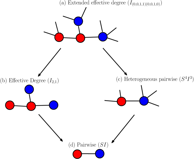
Figure 2: Illustration of the hierarchial structure of model recovery. Links that are known are given by lines and knowledge of a nodes status is given by circles. Susceptible and infective nodes are shown in blue and red respectively. The upper level (a) represents the extended effective degree ODEs. The status of the central node is known along with that of it’s neighbours and also their degrees. The secondary level is given by (b), the effective degree model where there is no knowledge of neighbours’ degrees and (c), the heterogenous pairwise model where the number of pairs of nodes and their relative degree is know. The final level shown, (d), is known as the standard pairwise model, [15], where the status of individual nodes and pairs is used.

5 Exactness of the models

In the previous sections we have at times referred to a set of ODEs as being exact. This terminology implies that the ODEs can be derived directly from the Kolmogorov equations which describe the evolution of the epidemic through the full state space $\mathcal{S}$ (on a network of size $N$, $\mathcal{S}=\{S,I\}^{N}$). In [23] the exactness of the pairwise equations was rigorously proven but no other motif structures were considered. In section 1, we conjectured that the newly defined exact effective degree model is derivable from the Kolmogorov equations. Due to the structure of the motifs used in the effective degree model a mechanistic proof (as in [23]) may be difficult and intricate to implement. Instead we will prove that a heuristic formulation of the ODEs for any motif structure is indeed exact providing they are written following rigorous bookkeeping. This derivation of the evolution equations for an arbitrary motif, directly from the Kolmogorv equations, will be based on an extension of ideas presented in [13] and [23] and using the notation defined in Tables 1 and 2.

We should note that in what follows a motif of connected nodes will only ever be counted once. In a network of size $N$ and considering a motif, $m$, with $k$ nodes this singular counting can be understood in the following way. We consider each of the $\binom{N}{k}$ unique sets of $k$ nodes between $1$ and $N$. Then for each set whose nodes are isomorphic in topological structure and status to the motif $m$, we simply increase the counter of such motifs by one. This formalism is unlike that used in the standard pairwise model where an $SS$ link would contribute a value of two to the $[SS]$ count. However, the two resultant sets of equations are equivalent in the sense that the different ways of counting can easily be recovered by using a simple mapping between the two. For this reason, whilst we prove that the following theorem is correct, it’s intricacy and generality means a certain amount of care is needed when interpreting the resultant terms. Using the notation defined in Table 2 the result for a general motif is then given in the following theorem.

Theorem 1

The equation for the expected number ($|\mathcal{M}|$) of motifs of type $\hat{m}$, given by

$$\dot{|\mathcal{M}|}= \tau\mathcal{N}_{in}^{SI}(\hat{m}^{-},\hat{m})+\tau\mathcal{N}_{ex}^{SI}(\hat{m}^{-},\hat{m})-\tau|\mathcal{M}|N_{in}^{SI}(\hat{m})-\tau\mathcal{N}_{ex}^{SI}(\hat{m})$$

$$+\gamma\mathcal{N}^{I}(\hat{m}^{+},\hat{m})-\gamma|\mathcal{M}|N^{I}(\hat{m})$$ (17)

is derivable directly from the exact Kolmogorov equations.

Table 1: Notation for matrix representation of the Kolmogorov equations (Table from [23]).

Variable	Definition
$N$	Number of nodes in the network
$G=(g_{ij})\in\{0,1\}^{N^{2}}$, $i,j=1,2,\ldots,N$	Adjacency matrix with $g_{ij}=1$ if nodes $i$ and $j$ are connected and $g_{ij}=0$ otherwise. The network is bi-directional and has no self loops such that $G=G^{T}$ and $G_{ii}=0$, $\forall$ $i$.
$\tau$	Rate of infection per ($S,I$) edge.
$\gamma$	Rate of recovery.
$\mathcal{S}=\{S,I\}^{N}$	State space of the network, with nodes either susceptible, $S$, or infected, $I$ and $|S|$ = $2^{N}$.
$\mathcal{S}^{k}=\{\mathcal{S}_{1}^{k},\mathcal{S}_{2}^{k},\ldots,\mathcal{S}_{c_{k}}^{k}\}$	The $c_{k}=\binom{N}{k}$ states with $k$ infected individuals in all possible configurations, with $k=0,1,\ldots,N$.
$X_{j}^{k}(t)$	Probability of being in state $\mathcal{S}_{j}^{k}$ at time $t$, where $k=0,1,\ldots,N$ and $j=1,2,\ldots,c_{k}$.
$X^{k}(t)$	$X^{k}(t)=\left(X_{1}^{k}(t),X_{2}^{k}(t),\ldots,X_{c_{k}}^{k}(t)\right)^{T}$.
$A^{k}_{i,j}$	Rate of transition from $\mathcal{S}_{j}^{k-1}$ to $\mathcal{S}_{i}^{k}$, where $k=0,1,\ldots,N$, $i=1,2,\ldots,c_{k}$ and $j=1,2,\ldots,c_{k-1}$ . Note that only one individual is changing (i.e. in this case an $S$ node changes to an $I$ through infection).
$C^{k}_{i,j}$	Rate of transition from $\mathcal{S}_{j}^{k+1}$ to $\mathcal{S}_{i}^{k}$, where $k=0,1,\ldots,N$, $i=1,2,\ldots,c_{k}$ and $j=1,2,\ldots,c_{k+1}$. Note that only one individual is changing (i.e. in this case an $I$ node changes to an $S$ through recovery).
$B^{k}_{i,j}$	Rate of transition from $\mathcal{S}_{j}^{k}$ to $\mathcal{S}_{i}^{k}$, where $B_{i,j}^{k}=0$ if $i\neq j$ with $k=0,1,\ldots,N$ and $i,j=1,2,\ldots,c_{k}$.

Table 2: Additional notation for matrix representation of the Kolmogorov equations

Variable	Definition
$\hat{m}$	An arbitrary motif encompassing both topology and status of nodes (e.g. an $S-I$ edge or a star like structure such as $I_{3,0}$). The arbitrary motif we are consdering which will encompass both topology and status of nodes.
$\hat{m}^{+}$	Represents the different motifs with the same structure as $\hat{m}$ but with a susceptible node of $\hat{m}$ having become infected.
$\hat{m}^{-}$	Represents the different motifs with the same structure as $\hat{m}$ but with with an infective node of $\hat{m}$ having become susceptible.
$M_{k,j}$	Set of $\hat{m}$ motifs in configuration state $\mathcal{S}_{j}^{k}$. Defining the $i^{th}$ element of $M_{k,j}$ as $\hat{m}_{k,j}^{i}$ gives $M_{k,j}=\{\hat{m}_{k,j}^{1},\hat{m}_{k,j}^{2},\ldots,\hat{m}_{k,j}^{|M|}\}$.
$M_{k,j}^{+}$	The set of motifs, in configuration state $\mathcal{S}_{j}^{k}$, with the same topology as $\hat{m}$ but with $1$ more infective and $1$ less susceptible. Defining the $i^{th}$ element of $M_{k,j}^{+}$ as $\hat{m}_{k,j}^{i+}$ gives $M_{k,j}^{+}=\{\hat{m}_{k,j}^{1+},\hat{m}_{k,j}^{2+},\ldots,\hat{m}_{k,j}^{|M_{k,j}^{+}|+}\}$.
$M_{k,j}^{-}$	The set of motifs, in configuration state $\mathcal{S}_{j}^{k}$, with the same topology as $\hat{m}$ but with $1$ less infective and $1$ more susceptible. Defining the $i^{th}$ element of $M_{k,j}^{-}$ as $\hat{m}_{k,j}^{i-}$ we have $M_{k,j}^{-}=\{\hat{m}_{k,j}^{1-},\hat{m}_{k,j}^{2-},\ldots,\hat{m}_{k,j}^{|M_{k,j}^{-}|-}\}$.
$N_{\hat{m}}(\mathcal{S}_{j}^{k})$	Number of $\hat{m}$ motifs in state $\mathcal{S}_{j}^{k}$, with $k=0,1,\ldots,N$ and $j=1,2,\ldots,c_{k}$.
$N_{in}^{SI}(\hat{h})$	Number of $SI$ links within the motif $\hat{h}$.
$\mathcal{N}_{in}^{SI}(\hat{h})$	Expected total number of $SI$ links within all motifs of type $\hat{h}$
$N_{in}^{SI}(\hat{h},k)$	Number of $SI$ links within the motif $\hat{h}$, along which, were an infection to occur, would result in a motif of type $k$.
$\mathcal{N}_{in}^{SI}(\hat{h},k)$	Expected total number of $SI$ links within all motifs of type $\hat{h}$, along which, were an infection to occur, would result in a motif of type $k$.
$N_{ex}^{SI}(\hat{h})$	Number of $SI$ links where the $S$ is contained within the motif $\hat{h}$ and the $I$ is external to it.
$\mathcal{N}_{ex}^{SI}(\hat{h})$	Expected total number of $SI$ links to all motifs with structure $\hat{h}$, where the $S$ is contained within the motif $\hat{h}$ and the $I$ external to it.
$N_{ex}^{SI}(\hat{h},k)$	Number of $SI$ links where the $S$ is contained within the motif $\hat{h}$ and the $I$ is external to it, along which, were an infection to occur, would result in a motif of type $k$.
$\mathcal{N}_{ex}^{SI}(\hat{h},k)$	Expected total number of $SI$ links to all motifs with structure $\hat{h}$, where the $S$ is contained within the motif $\hat{h}$ and the $I$ external to it, along which, were an infection to occur, would result in a motif of type $k$.
$N^{I}(\hat{h})$	Number of $I$ nodes within motif $\hat{h}$.
$N^{I}(\hat{h},k)$	Number of $I$ nodes within motif $\hat{h}$, whose recovery lead to a motif of type $k$.
$\mathcal{N}^{I}(\hat{h},k)$	Expected total number of $I$s within motifs of type $\hat{h}$, whose recovery lead to a motif of type $k$.

5.1 Proof of Theorem 1

For a detailed description of writing the Kolmogorov equations for an arbitrary graph we refer the reader to [13]. Here we only provide a brief description making use of the notation defined in Table 1. The $2^{N}$ elements of the state space, $\mathcal{S}=\{S,I\}^{N}$, can be divided into $N+1$ subsets where, for $0\leq k\leq N,\mathcal{S}^{k}$ is the subset of all states with $k$ infected nodes. Necessarily each subset contains $c_{k}=\binom{N}{k}$ distinct configurations, i.e.  $\mathcal{S}^{k}=(\mathcal{S}^{k}_{1},\mathcal{S}^{k}_{2},\ldots,\mathcal{S}^{k}_{c_{k}})$. The state of the system can only ever change in one of two ways, either via the infection of a node or via the recovery of a node. We can describe the evolution in the state space by a continuous time Markov-process. Setting $X^{k}_{j}(t)$ as the probability of the system being in state $\mathcal{S}_{j}^{k}$ at time $t$ and letting $X^{k}(t)=(X^{k}_{2}(t),X^{k}_{2}(t),\ldots,X^{k}_{c_{k}}(t)$ we can then write the Kolmogorov equations that capture the two possible transitions in the following matrix and vector form,

$$\dot{X}^{k}(t)=\begin{cases}B^{0}X^{0}+C^{0}X^{1}&\mbox{if }k=0,\\ A^{k}X^{k-1}+B^{k}X^{k}+C^{k}X^{k+1}&\mbox{for }1\leq k\leq N-1,\\ A^{N}X^{N-1}+B^{N}X^{N}&\mbox{if }k=N\end{cases}$$

Here the matrices $A^{k}$ capture the transitions into $\mathcal{S}^{k}$ via infection, $C^{k}$ capture the transitions into $\mathcal{S}^{k}$ via recovery and $B^{k}$ captures transitions within $\mathcal{S}^{k}$. Their entries are given as follows:

• $A^{k}_{i,j}$ is the rate of transition from $\mathcal{S}_{j}^{k-1}$ to $\mathcal{S}_{i}^{k}$, where $k=0,1,\ldots,N$, $i=1,2,\ldots,c_{k}$ and $j=1,2,\ldots,c_{k-1}$ . Note that none-zero entries of the matrix represent the transitions where only one individual is changing from susceptible to infected and the corresponding entrance will then equal $\tau$ multiplied by the number of infectious neighbours of the susceptible. These matrices encode the topological structure of the network.

• $C^{k}_{i,j}$ is the rate of transition from $\mathcal{S}_{j}^{k+1}$ to $\mathcal{S}_{i}^{k}$, where $k=0,1,\ldots,N$, $i=1,2,\ldots,c_{k}$ and $j=1,2,\ldots,c_{k+1}$. Note that none-zero entries of the matrix represent the transitions where only one individual is changing from infected to susceptible and the corresponding entrance will then equal $\gamma$.

• $B^{k}_{i,j}$ is the rate of transition from $\mathcal{S}_{j}^{k}$ to $\mathcal{S}_{i}^{k}$ where $B_{i,j}^{k}=0$ if $i\neq j$ with $k=0,1,\ldots,N$ and $i,j=1,2,\ldots,c_{k}$.

Letting $X(t)=(X^{0}(t),X^{1}(t),\ldots,X^{N}(t))^{T}$, we then write Kolmogorov equations in the following block tridiagonal form, $\dot{X}=PX$, where

$$P =\left(\begin{array}[]{cccccc}B^{0}&C^{0}&0&0&0&0\\ A^{1}&B^{1}&C^{1}&0&0&0\\ 0&A^{2}&B^{2}&C^{2}&0&0\\ 0&0&A^{3}&B^{3}&C^{3}&0\\ 0&0&\dots&\dots&\dots&0\\ 0&0&0&0&A^{N}&B^{N}\\ \end{array}\right).$$

From [13], we also know that the entries of the matrix $B$ are zero except on the diagonals, where we find that

$$B_{jj}^{k} =-\sum_{i=1}^{c_{k+1}}{A_{i,j}^{k+1}}-\sum_{i=1}^{c_{k-1}}{C_{i,j}^{k-1}}$$

$$=-\tau N_{SI}(S_{j}^{k})-k\gamma.$$ (18)

Where [13] focussed on individual and edge motifs here we focus on the derivation of evolution equations for the expected number of an arbitrary motif, $\hat{m}$. We begin by writing the exact equations for an arbitrary motif $\hat{m}$ based on the transition and recovery matrices. Using the notation from Table 2 this yields,

$$\dot{|\mathcal{M}|}= \sum_{k=0}^{N}{N_{\hat{m}}(S^{k})\dot{X}^{k}}$$

$$= N_{\hat{m}}(S^{0})\left[B^{0}X^{0}+C^{0}X^{1}\right]$$

$$+\sum_{k=1}^{N-1}N_{\hat{m}}(S^{k})\left[A^{k}X^{k-1}+B^{k}X^{k}+C^{k}X^{k+1}\right]$$

$$+N_{\hat{m}}(S^{N})\left[A^{N}X^{N-1}+B^{N}X^{N}\right]$$

$$= \sum_{k=1}^{N}N_{\hat{m}}(S^{k})A^{k}X^{k-1}+\sum_{k=0}^{N}N_{\hat{m}}(S^{k})B^{k}X^{k}+\sum_{k=0}^{N-1}N_{\hat{m}}(S^{k})C^{k}X^{k+1}$$

$$= \sum_{k=0}^{N-1}N_{\hat{m}}(S^{k+1})A^{k+1}X^{k}+\sum_{k=0}^{N}N_{\hat{m}}(S^{k})B^{k}X^{k}+\sum_{k=1}^{N}N_{\hat{m}}(S^{k-1})C^{k-1}X^{k}$$

$$= \left[N_{\hat{m}}(S^{1})A^{1}+N_{\hat{m}}(S^{0})B^{0}\right]X^{0}$$

$$+\sum_{k=1}^{N-1}\left[N_{\hat{m}}(S^{k+1})A^{k+1}+N_{\hat{m}}(S^{k})B^{k}+N_{\hat{m}}(S^{k-1})C^{k-1}\right]X^{k}$$

$$+\left[N_{\hat{m}}(S^{N})B^{N}+N_{\hat{m}}(S^{N-1})C^{N-1}\right]X^{N}.$$ (19)

Before continuing we note the following

$$B^{N} =B_{1,1}^{N}=-\sum_{i=1}^{N}C_{i,1}^{N-1}=-\gamma N,$$

$$B^{0} =B_{1,1}^{0}=-\sum_{i=1}^{N}A_{i,1}^{1}=-\tau N_{SI}(S_{1}^{0})=0.$$

Taking these and (18) into account and using the fact that $B$ is only none zero on it’s diagonal, we then obtain the following equation,

$$\dot{|\mathcal{M}|}= N_{\hat{m}}(S^{1})A^{1}X^{0}$$

$$+\sum_{k=1}^{N-1}\left[N_{\hat{m}}(S^{k+1})A^{k+1}-\tau\left(N_{\hat{m}}(S^{k})*N_{SI}(S^{k})\right)-\gamma kN_{\hat{m}}(S^{k})\right.+N_{\hat{m}}(S^{k-1})C^{k-1}\left.\right]X^{k}$$

$$+\left[N_{\hat{m}}(S^{N-1})C^{N-1}-\gamma NN_{\hat{m}}(S^{N})\right]X^{N}$$

$$= \sum_{k=1}^{N-1}\left[N_{\hat{m}}(S^{k+1})A^{k+1}-\tau\left(N_{\hat{m}}(S^{k})*N_{SI}(S^{k})\right)\right]X^{k}-\sum_{k=1}^{N}\left[\gamma kN_{\hat{m}}(S^{k})-N_{\hat{m}}(S^{k-1})C^{k-1}\right]X^{k}.$$ (20)

We note that the term containing $X^{0}$ vanishes because $A^{1}$ is a column vector with all zero entries. We now consider the summations involving the $A$ and $C$ matrices and the state $\mathcal{S}_{j}^{k}$. In this state there are $k$ infected and $N-k$ susceptible individuals. Without loss of generality the susceptible individuals are numbered $1$ to $N-k$ and the infected numbered from $N-k+1$ to $N$. Defining $r_{t}$ to be the number of infective neighbours of the node numbered $t$ we then obtain:

$$\left[N_{\hat{m}}(S^{k+1})A^{k+1}\right]_{j}= \sum_{i=1}^{c_{k+1}}N_{\hat{m}}(S_{i}^{k+1})A_{i,j}^{k+1}$$

$$\ = r_{1}\tau\left[N_{\hat{m}}(S_{j}^{k})+(\text{number of }\hat{m}\text{ gained by node }1\text{ becoming infected })\right.$$

$$\left.-(\text{number of }\hat{m}\text{ lost by node }1\text{ becoming infected })\right]$$

$$+ r_{2}\tau\left[N_{\hat{m}}(S_{j}^{k})+(\text{number of }\hat{m}\text{ gained by node }2\text{ becoming infected })\right.$$

$$\left.-(\text{number of }\hat{m}\text{ lost by node }2\text{ becoming infected })\right]$$

$$+ \ldots$$

$$+ r_{N-k}\tau\left[N_{\hat{m}}(S_{j}^{k})+(\text{number of }\hat{m}\text{ gained by node }(N-k)\text{ becoming infected })\right.$$

$$\left.-(\text{number of }\hat{m}\text{ lost by node }(N-k)\text{ becoming infected })\right]$$

$$= r_{1}\tau\left[N_{\hat{m}}(S_{j}^{k})+(\text{number of elements of }M_{k,j}^{-}\text{ where node }1\text{ is susceptible }\right.$$

$$\quad\quad\quad\quad\quad\text{and where node }1^{\prime}s\text{ infection would lead to a motif of type }\hat{m})$$

$$\left.-(\text{number of elements of }M_{k,j}\text{ where node }1\text{ is susceptible })\right]$$

$$+ r_{2}\tau\left[N_{\hat{m}}(S_{j}^{k})+(\text{number of elements of }M_{k,j}^{-}\text{ where node }2\text{ is susceptible }\right.$$

$$\quad\quad\quad\quad\quad\text{and where node }2^{\prime}s\text{ infection would lead to a motif of type }\hat{m})$$

$$\left.-(\text{number of elements of }M_{k,j}\text{ where node }2\text{ is susceptible })\right]$$

$$+ \ldots$$

$$+ r_{N-k}\tau\left[N_{\hat{m}}(S_{j}^{k})+(\text{number of elements of }M_{k,j}^{-}\text{ where node }(N-k)\text{ is susceptible }\right.$$

$$\quad\quad\quad\quad\quad\text{and where node }(N-k)^{\prime}s\text{ infection would lead to a motif of type }\hat{m})$$

$$\left.-(\text{number of elements of }M_{k,j}\text{ where node }(N-k)\text{ is susceptible })\right],$$

grouping the terms we obtain,

$$\left[N_{\hat{m}}(S^{k+1})A^{k+1}\right]_{j}= \tau N_{SI}(S_{j}^{k})N_{\hat{m}}(S_{j}^{k})+\tau\sum_{i=1}^{|M_{k,j}^{-}|}\left[N_{in}^{SI}(\hat{m}_{k,j}^{i-},\hat{m})+N_{ex}^{SI}(\hat{m}_{k,j}^{i-},\hat{m})\right]$$

$$- \tau|M_{k,j}|N_{in}^{SI}(\hat{m})-\tau\sum_{i=1}^{|M_{k,j}|}\left[N_{ex}^{SI}(\hat{m}_{k,j}^{i})\right].$$

Similarly,

$$\left[N_{\hat{m}}(S^{k-1})C^{k-1}\right]_{j}= \sum_{i=1}^{c_{k-1}}N_{\hat{m}}(S_{i}^{k-1})C_{i,j}^{k-1}$$

$$\ = \gamma\left[N_{\hat{m}}(S_{j}^{k})+(\text{number of }\hat{m}\text{ gained by node }(N-k+1)\text{ recovering })\right.$$

$$\left.-(\text{number of }\hat{m}\text{ lost by node }(N-k+1)\text{ recovering })\right]$$

$$+ \gamma\left[N_{\hat{m}}(S_{j}^{k})+(\text{number of }\hat{m}\text{ gained by node }(N-k+2)\text{ recovering })\right.$$

$$\left.-(\text{number of }\hat{m}\text{ lost by node }(N-k+2)\text{ recovering })\right]$$

$$+ \ldots$$

$$+ \gamma\left[N_{\hat{m}}(S_{j}^{k})+(\text{number of }\hat{m}\text{ gained by node }(N)\text{ recovering })\right.$$

$$\left.-(\text{number of }\hat{m}\text{ lost by node }(N)\text{ recovering })\right]$$

$$= \gamma\left[N_{\hat{m}}(S_{j}^{k})+(\text{number of elements of }M_{k,j}^{+}\text{ where node }(N-k+1)\text{ is infective }\right.$$

$$\quad\quad\quad\quad\quad\text{and where node }(N-k+1)^{\prime}s\text{ recovery would lead to a motif of type }\hat{m})$$

$$\left.-(\text{number of elements of }M_{k,j}\text{ of which node }(N-k+1)\text{ belongs })\right]$$

$$+ \gamma\left[N_{\hat{m}}(S_{j}^{k})+(\text{number of elements of }M_{k,j}^{+}\text{ where node }(N-k+2)\text{ is infective }\right.$$

$$\quad\quad\quad\quad\quad\text{and where node }(N-k+2)^{\prime}s\text{ recovery lead to a motif of type }\hat{m})$$

$$\left.-(\text{number of elements of }M_{k,j}\text{ of which node }(N-k+2)\text{ belongs })\right]$$

$$+ \ldots$$

$$+ \gamma\left[N_{\hat{m}}(S_{j}^{k})+(\text{number of elements of }M_{k,j}^{+}\text{ where node }(N)\text{ is infective }\right.$$

$$\quad\quad\quad\quad\quad\text{and where node }N^{\prime}s\text{ recovery would lead to a motif of type }\hat{m})$$

$$\left.-(\text{number of elements of }M_{k,j}\text{ of which node }(N)\text{ belongs })\right],$$

grouping the terms we obtain

$$\left[N_{\hat{m}}(S^{k-1})C^{k-1}\right]_{j}= \gamma kN_{\hat{m}}(S_{j}^{k})+\gamma\sum_{i=1}^{|M_{k,j}^{+}|}N^{I}(\hat{m}_{k,j}^{i+},\hat{m})-\gamma|M_{k,j}|\left(N^{I}(\hat{m})\right).$$

Defining

$$\mathcal{A}^{k+1}_{j} =\tau\sum_{i=1}^{|M_{k,j}^{-}|}\left[N_{in}^{SI}(\hat{m}_{k,j}^{i-},\hat{m})+N_{ex}^{SI}(\hat{m}_{k,j}^{i-},\hat{m})\right]-\tau|M_{k,j}|N_{in}^{SI}(\hat{m})-\tau\sum_{i=1}^{|M_{k,j}|}\left[N_{ex}^{SI}(\hat{m}_{k,j}^{i})\right]$$

$$\mathcal{C}^{k-1}_{j} =\gamma\sum_{i=1}^{|M_{k,j}^{+}|}\left[N^{I}(\hat{m}_{k,j}^{i+},\hat{m})\right]-\gamma|M_{k,j}|\left(N^{I}(\hat{m})\right)$$

and setting $\mathcal{A}^{k+1}=[{A}^{k+1}_{1},{A}^{k+1}_{j},\ldots,{A}^{k+1}_{c_{k}}]$ and $\mathcal{C}^{k-1}=[{C}^{k-1}_{1},{C}^{k-1}_{j},\ldots,{C}^{k-1}_{c_{k-1}}]$ yields,

$$\dot{|\mathcal{M}|}= \sum_{k=1}^{N-1}\left[N_{\hat{m}}(S^{k+1})A^{k+1}-\tau\left(N_{\hat{m}}(S^{K})*N_{SI}(S^{k})\right)\right]X^{k}-\sum_{k=1}^{N}\left[\gamma kN_{\hat{m}}(S^{k})-N_{\hat{m}}(S^{k-1})C^{k-1}\right]X^{k}$$

$$= \sum_{k=1}^{N-1}\left[\tau\left(N_{\hat{m}}(S^{K})*N_{SI}(S^{k})\right)+\mathcal{A}^{k+1}-\tau\left(N_{\hat{m}}(S^{K})*N_{SI}(S^{k})\right)\right]X^{k}-$$

$$\sum_{k=1}^{N}\left[\gamma kN_{\hat{m}}(S^{k})-\left(kN_{\hat{m}}(S^{k})+\mathcal{C}^{k-1}\right)\right]X^{k}$$

$$= \sum_{k=1}^{N-1}\left[\mathcal{A}^{k+1}\right]X^{k}+\sum_{k=1}^{N}\left[\mathcal{C}^{k-1}\right]X^{k}$$

$$= \sum_{k=1}^{N-1}\sum_{j=1}^{c_{k}}\mathcal{A}_{j}^{k+1}X_{j}^{k}+\sum_{k=1}^{N}\sum_{j=1}^{c_{k}}C_{j}^{k-1}X_{j}^{k}$$

$$= \sum_{k=1}^{N-1}\sum_{j=1}^{c_{k}}\left\{\tau\sum_{i=1}^{|M_{k,j}^{-}|}\left[N_{in}^{SI}(\hat{m}_{k,j}^{i-},\hat{m})+N_{ex}^{SI}(\hat{m}_{k,j}^{i-},\hat{m})\right]-\tau|M_{k,j}|N_{in}^{SI}(\hat{m})-\tau\sum_{i=1}^{|M_{k,j}|}\left[N_{ex}^{SI}(\hat{m}_{k,j}^{i})\right]\right\}X_{j}^{k}$$

$$+\sum_{k=1}^{N}\sum_{j=1}^{c_{k}}\left\{\gamma\sum_{i=1}^{|M_{k,j}^{+}|}\left[N^{I}(\hat{m}_{k,j}^{i+},\hat{m})\right]-\gamma|M_{k,j}|\left(N^{I}(\hat{m})\right)\right\}X_{j}^{k}$$

$$= \tau\mathcal{N}_{in}^{SI}(\hat{m}^{-},\hat{m})+\tau\mathcal{N}_{ex}^{SI}(\hat{m}^{-},\hat{m})-\tau|\mathcal{M}|N_{in}^{SI}(\hat{m})-\tau\mathcal{N}_{ex}^{SI}(\hat{m})$$

$$+\gamma\mathcal{N}^{I}(\hat{m}^{+},\hat{m})-\gamma|\mathcal{M}|N^{I}(\hat{m}).$$

Which matches equation 17 from Theorem 1. It is worth noting that our result is related to the equation for the “expectation of some average quantity” given in [21]. However, whilst the result in [21] is very general here we provide a proof by construction that, for a given motif, pinpoints the events that influence these motif and their rates.

5.2 Using the Theorem to prove the conjectured exact effective degree model is derivable from the Kolmogorov equations

Letting $\hat{m}$ be an $S_{s,i}$-type motif from the effective degree model earlier and using Theorem $1$, we find that the exact equations can be written as

$$\frac{dS_{s,i}}{dt}= \tau\mathcal{N}_{in}^{SI}(\hat{m}^{-},\hat{m})+\tau\mathcal{N}_{ex}^{SI}(\hat{m}^{-},\hat{m})-\tau|\mathcal{M}|N_{in}^{SI}(\hat{m})-\tau\mathcal{N}_{ex}^{SI}(\hat{m})$$

$$+\gamma\mathcal{N}^{I}(\hat{m}^{+},\hat{m})-\gamma|\mathcal{M}|N^{I}(\hat{m})$$

$$= \tau\times\left(\text{the total expected number of SI connections within }S_{s+1,i-1}\text{-type motifs}\right.$$

$$\quad\quad\text{where if infection occurs we obtain a }S_{s,i}\text{-type motif}\left.\right)$$

$$+\tau\times\left(\text{the total expected number of SI connections where S lies within}\right.$$

$$\quad\quad\quad S_{s+1,i-1}\text{-type motifs and the I is external to the given motif}$$

$$\quad\quad\quad\text{and where, were an infection to occur, we obtain a }S_{s,i}\text{-type motif}\left.\right)$$

$$-\tau S_{s,i}\times\left(\text{number of SI connections within an individual }S_{s,i}\text{-type motifs}\right)$$

$$-\tau\times\left(\text{the total expected number of SI connections where S belongs to }\right.$$

$$\quad\quad\quad S_{s,i}\text{-type motifs and the I is external to the given motif}\left.\right)$$

$$+\gamma\times\left(\text{the total expected number I's within }S_{s-1,i+1}\text{-type and }I_{s,i}\text{-type motifs}\right.$$

$$\quad\quad\quad\text{where there recovery would give a }S_{s,i}\text{-type motif}\left.\right)$$

$$-\gamma S_{s,i}\times\left(\text{number of I within an individual }S_{s,i}\text{-type motif}\right)$$

$$= \tau\left[ISS_{s+1,i-1}\right]-\tau iS_{s,i}-\tau\left[ISS_{s,i}\right]+\gamma I_{si}+\gamma(i+1)S_{s-1,i+1}-\gamma iS_{s,i}$$

which is indeed the conjectured exact equation for $S_{s,i}$ (similar derivation holds for $I_{s,i}$). To clarify the above derivation we note that a term such as $\tau\mathcal{N}_{in}^{SI}(\hat{m}^{-},\hat{m})$ will make no contribution to the resultant equation as there are no internal $SI$ connections within $S_{s-1,i+1}$-type motifs along which an infection would lead to an $S_{s,i}$-type motif. However other terms, such as $\tau\mathcal{N}_{ex}^{SI}(\hat{m}^{-},\hat{m})$, have a direct correspondence with the resultant output (in this case the $\tau\left[ISS_{s+1,i-1}\right]$ term).

6 Comparison of the closed models

In comparing the models the obvious question to ask is when does one model perform better than another, i.e. which model approximates better or more accurately the simulation results or the solution of the Kolmogorov/master equations where solvable. As discussed earlier, the pairwise model is known to perform well on networks that are well characterised by the average degree (i.e. regular random and Erdős-Rényi graphs). What is less known is under what circumstances do the heterogenous pairwise and effective degree models outperform one another.

To assess the performance of the three closed models we compared individual simulations to the solutions of the ODE’s on four different types of undirected network. For each of the different types of networks we used the Gillespie algorithm, [8], to run $500$ simulations on networks of size $N=500$ ($1$ simulation on $500$ different randomly generated networks). The results of these simulations were then averaged to obtain an expected value to compare to the solution of the various ODE’s. We began by considering regular random networks where all nodes have the same number of randomly chosen neighbours and then Erdős-Rényi random networks where the distribution of degrees converges to a Poisson distribution. Figure 3 plots simulation results against the different solutions of the ODEs for these two networks. On the regular network, whilst the two different pairwise models and the effective degree offer an improvement in performance over the standard meanfield equations, there is little to distinguish between the improved approaches. As expected, on the Erdős-Rényi random networks, the pairwise model improves on the meanfield model and, in turn, the effective degree and heterogeneous pairwise models improve even further on this. Again, however, there is little to distinguish between effective degree and the heterogeneous pairwise models.

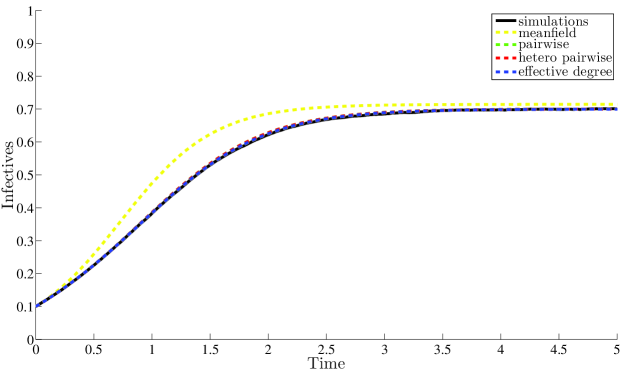
(a) Regular random

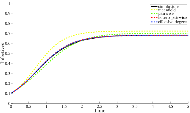
(b) Erdos-Renyi

Figure 3: ODE performance on different networks Each network is of size $N=500$ and with disease parameters given by $\gamma=1$ and $\tau=0.5$. Average prevalence was calculated from individual simulations on $500$ different networks. Initial conditions for the ODEs were obtained by averaging the initial conditions from each of the simulations. (a) Regular random network, each node having degree $7$. (b) Erdős-Rényi random network with average degree $7$.

To investigate further we ran simulations on networks exhibiting greater heterogeneity in their degree distribution. Firstly we considered networks with degrees between $1$ and $25$ chosen from a powerlaw degree distribution ($p(x)=Ax^{-1.5}$) and generated by the configuration model algorithm [20]. Networks with scale-free like degree distributions may be more closely related to those of real world networks ([4]) and may thus be of greater use in understanding the applicability of more theoretical modelling approaches. Secondly we considered graphs with the same power law degree distributions as before but this time rewired based on the “greedy” assortativity algorithm (discussed in [25]). This rewiring leads to an increase in the assortativity coefficient ([19]) which measures the propensity of nodes of similar degrees to attach to one another. In theory, we should be able to capture this correlation with the heterogenous pairwise equations as they explicitly take the degree of connected nodes into account within the initial conditions. The results are illustrated in Figure 4.

Whilst on the powerlaw network network there is little difference between heterogeneous pairwise and effective degree when the assortativity is increased, there is a clear improvement in the performance of the heterogenous pairwise model over the effective degree. Any performance benefit must, however, be considered in terms of the model complexity given in table 3 (note that in this table $M$ is the maximum possible degree in the network and we given the minimum number of equations needed to implement the ODEs).

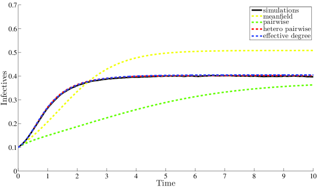
(a) Power-law

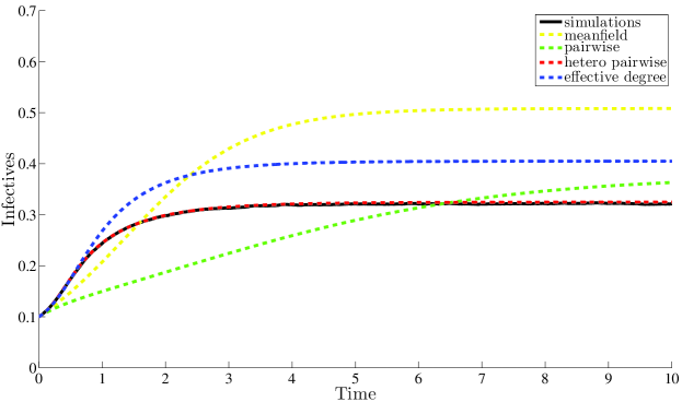
(b) Assortative power-law

Figure 4: ODE performance on different networks. Each network is of size $N=500$ and with disease parameters given by $\gamma=1$ and $\tau=0.5$. Average prevalence was calculated from individual simulations on $500$ different networks. Initial conditions for the ODEs were obtained by averaging the initial conditions from each of the simulations. (a) Network with degrees chosen from a power law distribution (b) Networks with degrees chosen from a powerlaw distribution but rewired to have assortativity coefficient $r\approx 0.49$.

Table 3: Complexity of closed ODEs

Model	# equations	complexity
meanfield	$1$	$\mathcal{O}(1)$
pairwise	$3$	$\mathcal{O}(1)$
effective degree	$M(M+3)-1$	$\mathcal{O}(M^{2})$
heterogeneous pairwise	$2M(M+1)-1$	$\mathcal{O}(M^{2})$
Kolmogorov equations	$2^{N}$	$\mathcal{O}(2^{N})$

A final comparison between the performance of the different closed models is to look at their rate of convergence to the solution of the Kolmogorov equations on a complete (fully connected) network. On a complete network it is possible (see [13]) to reduce the full system of $2^{N}$ equations to just $N+1$ equations. This allows us to compare the true solution to the approximate solution of the meanfield, pairwise (equivalent to heterogenous pairwise on a complete graph) and effective degree models. Interestingly we find that all three exhibit $O(1/N)$ convergence, where although both pairwise and effective degree bring an improvement on meanfield, the difference between the convergence of the two is neglible and almost indecernible (see figure 5).

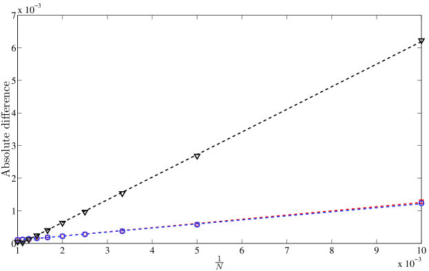
Figure 5: Convergence to exact solution on a complete graph. Absolute difference between the exact steady state solution of the percentage of infected individuals and those calculated from three different ODE models for $10$ different network sizes and initial prevalence of $40$ percent. Black triangles represent meanfield, blue circles effective degree and red squares the pairwise equations. Linear lines of best fit are also shown. This shows that the error(N) appears to be of O(1/N) as N tends to infinity.

7 Discussion

In this paper we set out to achieve a greater understanding of the relation between some of the more common approaches to modelling disease dynamics. In doing so we conjectured an exact version of the effective degree model [17] and showed how this model could be used to recover the pairwise model [15]. We then extended this model to incorporate greater network structure and illustrated how, from this extension, we could then recover the heterogeneous pairwise model [7]. We then proved that the conjectured exact effective degree model was indeed exact by proving that a heuristic derivation of an ODE model for an arbitrary motif was derivable directly from the Kolmogorov equations and noting that the exact effective degree model was just a particular case of this heuristic model. Finally we considered the performance of the different models on four different type of networks and have analysed numerically the rate of convergence to the lumped Kolmogorov equations on a complete network. These comparisons suggest a performance hierarchy of models as illustrated in Figure 6 and it is worth noting that the performance benefit of the heterogenous pairwise model on networks exhibiting susceptible $\rightarrow$ infectious $\rightarrow$ removed (SIR) disease dynamics was also touched upon in [5].

Whilst we have shown how current models can be extended in a way that can capture more network topology, these extensions have a more theoretical rather than practical motivation as their added complexity makes them not only less tractable but also more resource intensive in their solving, thus making the use of simulations more of an attractive proposition. As the links between these models are better understood, future work will likely focus on the following three areas. Firstly, a more realistic network will have a more clique-like structure. For example an individual is likely a member of a household in which he has regular contacts within and less regular contacts outside. Being able to incorporate this household structure within epidemic models is thus important in understanding the outbreak and necessary curtailment of an infectious disease (see [3, 11, 24]). Secondly, a network of individuals is not well represented by a static network. An individual may have regular contact with few individuals but may create or break contacts with others in ways that a static network representation cannot capture. For this reason it is important to take into consideration not only the dynamics of the disease but also the dynamics of the network and how the two impact on one another (see [9, 14]). Thirdly, assuming we can write down exact differential equations we have to close them in some way. Understanding the performance of current, and also the derivation of new closures, is arguably the most important task ahead as it is the closures that limit the performance of any system of ODEs.

Figure 6: Model performance hierarchy. Model performance hierarchy based on our observations. Here K represents the Kolmogorov equations and HetPW the heterogeneous pairwise equations.

Appendix $1$

Illustration of the exact effective degree transitions where the central node is infective.

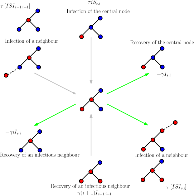
Figure 7: Illustration of the transitions into and out of the $I_{2,1}$ class. Susceptible nodes are given in blue and infective nodes in red. Transitions into and out of the class are shown in grey and green, respectively. The corresponding terms of the general equation are also given.

Appendix $2$

Derivation of the pairwise equation from the exact effective degree model for singles and pairs are as follows,

$$\frac{d}{dt}\left[S\right] =\sum_{s,i}\dot{S}_{s,i}=\gamma\left[I\right]-\tau\left[SI\right],$$

$$\frac{d}{dt}\left[I\right] =\sum_{s,i}\dot{I}_{s,i}=-\gamma\left[I\right]+\tau\left[SI\right],$$

where most terms from the original effective degree equations cancel and we have used that $\sum_{s,i}iS_{s,i}=[SI]$ and $\sum_{s,i}I_{s,i}=[I]$. For the pairs the effective degree model yields,

$$\frac{d}{dt}\left[SS\right]= \sum_{s,i}s\dot{S}_{si}$$

$$= -\tau\sum{siS_{s,i}}+\gamma\sum{sI_{s,i}}+\gamma\sum{s(i+1)S_{s-1,i+1}}-\gamma\sum{isS_{s,i}}$$

$$+\tau\sum{s[ISS_{s+1,i-1}]}-\tau\sum{s[ISS_{s,i}]}$$

$$= -\tau[ISS]+\gamma[IS]+\gamma\sum{(s-1)(i+1)S_{s-1,i+1}}+\gamma\sum{(i+1)S_{s-1,i+1}}$$

$$-\gamma[ISS]+\tau\sum{(s+1)[ISS_{s+1,i-1}]}-\tau\sum{[ISS_{s+1,i-1}]}-\tau\sum{s[ISS_{s,i}]}$$

$$= -\tau[ISS]+\gamma[IS]+\gamma[ISS]+\gamma[IS]-\gamma[ISS]-\tau[ISS]$$

$$= -2\tau[ISS]+2\gamma[IS],$$

$$\frac{d}{dt}\left[SI\right]= \sum_{s,i}s\dot{I}_{si}$$

$$= \tau\sum{siS_{s,i}}-\gamma\sum{sI_{s,i}}+\gamma\sum{s(i+1)I_{s-1,i+1}}-\gamma\sum{siI_{s,i}}$$

$$+\tau\sum{s[ISI_{s+1,i-1}]}-\tau\sum{s[ISI_{s,i}]}$$

$$= \tau[ISS]-\gamma[IS]+\gamma\sum{(s-1)(i+1)I_{s-1,i+1}}+\gamma\sum{(i+1)I_{s-1,i+1}}$$

$$-\gamma[IIS]+\tau\sum{(s+1)[ISI_{s+1,i-1}]}-\tau\sum{[ISI_{s+1,i-1}]}-\tau\sum{s[ISI_{s,i}]}$$

$$= \tau[ISS]-\gamma[IS]+\gamma[IIS]+\gamma[II]-\gamma[IIS]-\tau([ISI]+[IS])$$

$$= \tau\left([ISS]-[ISI]-[IS]\right)+\gamma\left([II]-[IS]\right),$$

$$\frac{d}{dt}\left[II\right]= \sum_{s,i}i\dot{I}_{si}$$

$$= \tau\sum{i^{2}S_{s,i}}-\gamma\sum{iI_{s,i}}+\gamma\sum{i(i+1)I_{s-1,i+1}}-\gamma\sum{i^{2}I_{s,i}}$$

$$+\tau\sum{i[ISI_{s+1,i-1}]}-\tau\sum{i[ISI_{s,i}]}$$

$$= \tau\sum{i(i-1)S_{s,i}}+\tau\sum{iS_{s,i}}-\gamma[II]$$

$$+\gamma[III]-\gamma\sum{i(i-1)I_{s,i}}-\gamma\sum{iI_{s,i}}$$

$$+\tau\sum{(i-1)[ISI_{s+1,i-1}]}+\tau\sum{[ISI_{s+1,i-1}]}-\tau\sum{i[ISI_{s,i}]}$$

$$= \tau[ISI]+\tau[IS]-\gamma[II]+\gamma[III]-\gamma[III]-\gamma[II]+\tau[ISI]+\tau[IS]$$

$$= 2\tau\left([ISI]+[IS]\right)-2\gamma[II].$$

Appendix $3$

Derivation of the heterogeneous pairwise equations from the effective degree with neighbourhood composition model. For singles and pairs the following identities hold,

$$\frac{d}{dt}\left[S^{n}\right] =\sum_{|s^{\prime}|+|i^{\prime}|=N}\dot{S}_{s^{\prime},i^{\prime}}=\gamma\left[I^{n}\right]-\tau\left[S^{n}I\right],$$

$$\frac{d}{dt}\left[I^{n}\right] =\sum_{|s^{\prime}|+|i^{\prime}|=N}\dot{I}_{s^{\prime},i^{\prime}}=-\gamma\left[I^{n}\right]+\tau\left[S^{n}I\right],$$

$$\frac{d}{dt}\left[S^{l}S^{n}\right]= \sum_{|s^{\prime}|+|i^{\prime}|=n}{s_{l}\dot{S}_{s^{\prime},i^{\prime}}}$$

$$= -\tau\sum{s_{l}|i^{\prime}|S_{s^{\prime},i^{\prime}}}+\gamma\sum{s_{l}I_{s^{\prime},i^{\prime}}}+\gamma\sum{s_{l}\sum_{k=1}^{M}{(i_{k}+1)S_{s^{\prime}_{k-},i^{\prime}_{k+}}}}$$

$$-\gamma\sum{s_{l}|i^{\prime}|S_{s^{\prime},i^{\prime}}}+\tau\sum{s_{l}\sum_{k=1}^{M}{\left[IS^{k}S_{s^{\prime}_{k+},i^{\prime}_{k-}}\right]}-\tau\sum{s_{l}\left[ISS_{s^{\prime},i^{\prime}}\right]}}$$

$$= -\tau\left[IS^{n}S^{l}\right]+\gamma\left[S^{l}I^{n}\right]+\gamma\sum{s_{l}\sum_{k\neq l}{(i_{k}+1)S_{s^{\prime}_{k-},i^{\prime}_{k+}}}}$$

$$+\gamma\sum{(s_{l}-1)(i_{l}+1)S_{s^{\prime}_{l-},i^{\prime}_{l+}}}+\gamma\sum{(i_{l}+1)S_{s^{\prime}_{l-},i^{\prime}_{l+1}}}-\gamma\left[IS^{n}S^{l}\right]$$

$$+\tau\sum{s_{l}\sum_{k\neq l}{\left[IS^{k}S_{s^{\prime}_{k+},i^{\prime}_{k-}}\right]}+\tau\sum{(s_{l}+1)\left[IS^{l}S_{s^{\prime}_{l+},i^{\prime}_{l-}}\right]}}$$

$$-\tau\sum{\left[IS^{l}S_{s^{\prime}_{l+},i^{\prime}_{l-}}\right]-\tau\sum{s_{l}\left[ISS_{s^{\prime},i^{\prime}}\right]}}$$

$$= -\tau\left[IS^{n}S^{l}\right]+\gamma\left[S^{l}I^{n}\right]+\gamma\left[S^{l}S^{n}I\right]+\gamma\left[I^{l}S^{n}\right]$$

$$-\gamma\left[IS^{n}S^{l}\right]-\tau\left[IS^{l}S^{n}\right]$$

$$= -\tau\left[IS^{n}S^{l}\right]-\tau\left[IS^{l}S^{n}\right]+\gamma\left[S^{l}I^{n}\right]+\gamma\left[I^{l}S^{n}\right],$$

$$\frac{d}{dt}\left[S^{l}I^{n}\right]= \sum_{|s^{\prime}|+|i^{\prime}|=n}{s_{l}\dot{I}_{s^{\prime},i^{\prime}}}$$

$$= \tau\sum{s_{l}|i^{\prime}|S_{s^{\prime},i^{\prime}}}-\gamma\sum{s_{l}I_{s^{\prime},i^{\prime}}}+\gamma\sum{s_{l}\sum_{k=1}^{M}{(i_{k}+1)I_{s^{\prime}_{k-},i^{\prime}_{k+}}}}$$

$$-\gamma\sum{s_{l}|i^{\prime}|I_{s^{\prime},i^{\prime}}}+\tau\sum{s_{l}\sum_{k=1}^{M}{\left[IS^{k}I_{s^{\prime}_{k+},i^{\prime}_{k-}}\right]}}-\tau\sum{s_{l}\left[ISI_{s^{\prime},i^{\prime}}\right]}$$

$$= \tau\left[IS^{n}S^{l}\right]-\gamma\left[S^{l}I^{n}\right]+\gamma\sum{s_{l}\sum_{k\neq l}{(i_{k}+1)I_{s^{\prime}_{k-},i^{\prime}_{k+}}}}$$

$$+\gamma\sum{(s_{l}-1)(i_{l}+1)I_{s^{\prime}_{l-},i^{\prime}_{l+}}}+\gamma\sum{(i_{l}+1)I_{s^{\prime}_{l-},i^{\prime}_{l+1}}}-\gamma\left[II^{n}S^{l}\right]$$

$$+\tau\sum{s_{l}\sum_{k\neq l}{\left[IS^{k}I_{s^{\prime}_{k+},i^{\prime}_{k-}}\right]}}+\tau\sum{(s_{l}+1)\left[IS^{l}I_{s^{\prime}_{l+},i^{\prime}_{l-}}\right]}$$

$$-\tau\sum{\left[IS^{l}I_{s^{\prime}_{l+},i^{\prime}_{l-}}\right]}-\tau\sum{s_{l}\left[ISI_{s^{\prime},i^{\prime}}\right]}$$

$$= \tau\left[IS^{n}S^{l}\right]-\gamma\left[S^{l}I^{n}\right]+\gamma\left[S^{l}I^{n}I\right]+\gamma\left[I^{l}I^{n}\right]$$

$$-\gamma\left[II^{n}S^{l}\right]-\tau\left[IS^{l}I^{n}\right]-\tau\left[S^{l}I^{n}\right]$$

$$= \tau\left[IS^{n}S^{l}\right]-\tau\left[IS^{l}I^{n}\right]-\tau\left[S^{l}I^{n}\right]+\gamma\left[I^{l}I^{n}\right]-\gamma\left[S^{l}I^{n}\right],$$

$$\frac{d}{dt}\left[I^{l}I^{n}\right]= \sum_{|s^{\prime}|+|i^{\prime}|=n}{i_{l}\dot{I}_{s^{\prime},i^{\prime}}}$$

$$= \tau\sum{i_{l}|i^{\prime}|S_{s^{\prime},i^{\prime}}}-\gamma\sum{i_{l}I_{s^{\prime},i^{\prime}}}+\gamma\sum{i_{l}\sum_{k=1}^{M}{(i_{k}+1)I_{s^{\prime}_{k-},i^{\prime}_{k+}}}}$$

$$-\gamma\sum{i_{l}|i^{\prime}|I_{s^{\prime},i^{\prime}}}+\tau\sum{i_{l}\sum_{k=1}^{M}{\left[IS^{k}I_{s^{\prime}_{k+},i^{\prime}_{k-}}\right]}}-\tau\sum{i_{l}\left[ISI_{s^{\prime},i^{\prime}}\right]}$$

$$= \tau\sum{i_{l}\left(|i^{\prime}|-1\right)S_{s^{\prime},i^{\prime}}}+\tau\sum{i_{l}S_{s^{\prime},i^{\prime}}}-\gamma\left[I^{l}I^{n}\right]$$

$$+\gamma\left[I^{l}I^{n}I\right]-\gamma\sum{i_{l}\left(|i^{\prime}|-1\right)I_{s^{\prime},i^{\prime}}}-\gamma\sum{i_{l}I_{s^{\prime},i^{\prime}}}$$

$$+\tau\sum{i_{l}\sum_{k\neq l}{\left[IS^{k}I_{s^{\prime}_{k+},i^{\prime}_{k-}}\right]}}+\tau\sum{\left(i_{l}-1\right)\left[IS^{l}I_{s^{\prime}_{l+},i^{\prime}_{l-}}\right]}$$

$$+\tau\sum{\left[IS^{l}I_{s^{\prime}_{l+},i^{\prime}_{l-}}\right]}-\tau\sum{i_{l}\left[ISI_{s^{\prime},i^{\prime}}\right]}$$

$$= \tau\left[I^{l}S^{n}I\right]+\tau\left[I^{l}S^{n}\right]-2\gamma\left[I^{l}I^{n}\right]$$

$$+\gamma\left[I^{l}I^{n}I\right]-\gamma\left[I^{l}I^{n}I\right]+\tau\left[IS^{l}I^{n}\right]+\tau\left[S^{l}I^{n}\right]$$

$$= \tau\left[I^{l}S^{n}I\right]+\tau\left[I^{l}S^{n}\right]-2\gamma\left[I^{l}I^{n}\right]+\tau\left[IS^{l}I^{n}\right]+\tau\left[S^{l}I^{n}\right].$$

References

- [1] L.J. Allen. Introduction to stochastic epidemic models. In Mathematical Epidemiology [Lecture Notes in Mathematics, vol 1945], Springer, Berlin. 81-130 (2008).
- [2] R.M. Anderson & R.M. May. Infectious diseases of humans: dynamics and control. Oxford University Press (1999).
- [3] F. Ball, D. Sirl & P. Trapman. Analysis of a stochastic SIR epidemic on a random network incorporating household structure. Math. Biosci. 224, 2, 53-73 (2010).
- [4] A.-L. Barabási. Scale-Free Networks: A Decade and Beyond. Science, 325 (5939), 412-413 (2009).
- [5] L. Danon, A.P. Ford, T. House, et al. Networks and the Epidemiology of Infectious Disease. Interdisciplinary Perspectives on Infectious Diseases, vol. 2011 (2011)
- [6] O. Diekmann & J.A.P. Heesterbeek. Mathematical epidemiology of infectious diseases: model building, analysis and interpretation. Wiley, Chichester.
- [7] K.T.D. Eames &M.J. Keeling. Modelling dynamic and network heterogeneneities in the spread of sexually transmitted diseases. Proc. Natl Acad. Sci. USA 99, 13330 13335 (2002).
- [8] D.T. Gillespie. Exact stochastic simulation of coupled chemical reactions. J. Phys. Chem. 81(25), 2340-2361 (1977).
- [9] T. Gross, C.D. D’Lima & B. Blasius. Epidemic dynamics on an adaptive network. Phys. Rev. Letters 96, 208701-4 (2006)
- [10] C. Hadjichrysanthou, M. Broom & I.Z. Kiss. Approximating evolutionary dynamics on networks using a neighbourhood configuration model. J. Theor. Biol. 312, 13-21 (2012).
- [11] T. House, M.J. Keeling. Deterministic epidemic models with explicit household structure. Math. Biosci. 213, 29-39 (2008).
- [12] T. House, G. Davies, L. Danon & M.J. Keeling. A motif-based approach to network epidemics. Bulletin of Mathematical Biology, 71, 1693-1706 (2009).
- [13] P.L. Simon, M. Taylor & I.Z. Kiss. Exact epidemic models on graphs using graph-automorphism driven lumping. J. Math. Biol. 62, 479-508 (2011).
- [14] I.Z. Kiss, L. Berthouze, T.J. Taylor & P.L. Simon. Modelling approaches for simple dynamic networks and applications to disease transmission models. Proc. R. Soc. A. 468, 1332 (2012).
- [15] M.J. Keeling. The effects of local spatial structure on epidemiological invasions. Proc. R. Soc. Lond. B 266, 859-867 (1999).
- [16] E. Kenah & J.C. Miller. Epidemic percolation networks, epidemic outcomes, and interventions. Interdisciplinary Perspectives on Infectious Diseases, 2011, (2011).
- [17] J. Lindquist, J. Ma, P. van den Driessche & F.H. Willeboordse. Effective degree network disease models. J. Math. Biol. 62, 143-164 (2011).
- [18] V. Marceau, P. Noel, L. H bert-Dufresne, A. Allard & L.J. Dub . Adaptive networks: Coevolution of disease and topology. Phys. Rev. E 82, 036116 (2010).
- [19] M.E.J. Newman. Mixing patterns in networks. Phys. Rev. E 67, 026126 (2003).
- [20] M.E.J. Newman. The structure and function of complex networks. SIAM Rev. 45, 167-256 (2003).
- [21] D.A. Rand. Correlation equations and pair approximations for spatial ecologies in Advanced Ecological Theory: principles and applications, Edited by Jacqueline McGlade. Blackwell Science (1999).
- [22] K. Sharkey. Deterministic epidemiological models at the individual level. J. Math. Biol. 57, 311-331 (2008).
- [23] M. Taylor, P.L. Simon, D.M. Green, T. House & I.Z. Kiss. From Markovian to pairwise epidemic models and the performance of moment closure approximations. J. Math. Biol. 64, 1021-1042 (2012).
- [24] E. Volz, J.C. Miller, A. Galvani, L.A. Meyers. Effects of Heterogeneous and Clustered Contact Patterns on Infectious Disease Dynamics. PLoS Comput. Biol. 7(6), e1002042 (2011)
- [25] W. Winterbach, D. de Ridder, H.J. Wang, M. Reinders & P. Van Mieghem. Do greedy assortativity optimization algorithms produce good results? Eur. Phys. J. B 85: 151 (2012)