A Generalized Finite element method
for the displacement obstacle problem of
Clamped Kirchhoff plates

Abstract.

A generalized finite element method for the displacement obstacle problem of clamped Kirchhoff plates is considered in this paper. We derive optimal error estimates and present numerical results that illustrate the performance of the method.

1. Introduction

Let $\Omega$ be a bounded polygonal domain $\Omega\subset\mathbb{R}^{2}$, $f\in L_{2}(\Omega)$, $g\in H^{4}(\Omega)$, and $\psi_{1},\psi_{2}\in C^{2}(\Omega)\cap C(\bar{\Omega})$ be two obstacle functions such that

(1.1) $$\psi_{1}<\psi_{2}\;\;\text{in}\;\;\Omega\quad\text{and}\quad\psi_{1}<g<\psi_{2}\;\;\text{on}\;\partial\Omega.$$

Consider the following problem: Find $u\in H^{2}(\Omega)$ such that

(1.2) $$u=\mathop{\rm argmin}_{v\in K}G(v),$$

where

(1.3) $$K =\{v\in H^{2}(\Omega):\,u-g\in H^{2}_{0}(\Omega),\;\psi_{1}\leq v\leq\psi_{2}\;\text{on}\;\Omega\},$$

(1.4) $$G(v) =\frac{1}{2}a(v,v)-(f,v),$$

(1.5) $$a(v,w) =\int_{\Omega}\nabla^{2}v:\nabla^{2}w\,dx,\quad(f,v)=\int_{\Omega}fv\,dx$$

and $\nabla^{2}v:\nabla^{2}w=\sum_{i,j=1}^{2}v_{x_{i}x_{j}}w_{x_{i}x_{j}}$ is the (Frobenius) inner product of the Hessian matrices of $v$ and $w$.

Since $K$ is a nonempty closed convex subset of $H^{2}(\Omega)$ and $a(\cdot,\cdot)$ is symmetric and coercive on $H^{2}_{0}(\Omega)$ which contains the set $K-K$, it follows from the standard theory [28, 23, 26, 22] that (1.2) has a unique solution $u\in K$ characterized by the following variational inequality:

(1.6) $$a(u,v-u)\geq(f,v-u)\qquad\forall\,v\in K.$$

The convergence of finite element methods for second order obstacle problems was investigated in [19, 13, 14], shortly after it was shown in [11] that the solutions for such obstacle problems belong to $H^{2}(\Omega)$ under appropriate regularity assumptions on the data. This full elliptic regularity allows the complementarity form of the variational inequality (in the strong sense) to be used in the convergence analysis.

In contrast, it was shown in [20, 21, 15] that the solution $u$ of (1.2)/(1.6) belongs to $H^{3}_{loc}(\Omega)\cap C^{2}(\Omega)$ under the assumptions above on $f$, $g$, $\psi_{1}$ and $\psi_{2}$. Since the obstacles are separated from each other and from the displacement boundary condition (cf. (1.1)), we have $\Delta^{2}u=f$ near $\partial\Omega$. Therefore it follows from the elliptic regularity theory for the biharmonic operator on polygonal domains [5, 24, 16, 27] that $u\in H^{2+\alpha}(\mathcal{N})$ for some $\alpha\in(\frac{1}{2},1]$ in an open neighborhood $\mathcal{N}$ of $\partial\Omega$. The elliptic regularity index $\alpha$ is determined by the interior angles of $\Omega$ and we can take $\alpha$ to be $1$ for convex $\Omega$. Thus the solution $u$ of (1.2)/(1.6) belongs to $H^{2+\alpha}(\Omega)\cap H^{3}_{loc}(\Omega)\cap C^{2}(\Omega)$ in general. Moreover, it is easy to construct examples where $u\notin H^{4}_{loc}(\Omega)$ even for smooth data [15].

This lack of $H^{4}_{loc}(\Omega)$ regularity means that the complementarity form of (1.6) only exists in a weak sense [15]. Consequently convergence analysis based on the weak complementarity form of (1.6) would only lead to suboptimal error estimates.

A new convergence analysis for finite element methods for (1.2)/(1.6) that does not rely on the complementarity form of the variational inequality (1.6) was proposed in [10], where optimal convergence was established for $C^{1}$ finite element methods, classical nonconforming finite element methods, and $C^{0}$ interior penalty methods for clamped plates ($g=0$) on convex domains. The results in [10] were subsequently extended to general polygonal domains and general Dirichlet boundary conditions for a quadratic $C^{0}$ interior penalty method [9] and a Morley finite element method [8]. The goal of this paper is to extend the results in [9, 8] to a generalized finite element method for plates [17, 31].

The rest of the paper is organized as follows. We introduce the generalized finite element method in Section 2 and carry out the convergence analysis in Section 3. Numerical results are reported in Section 4.

2. A Generalized Finite Element Method

We begin with the construction of the approximation space $V_{h}$ in Section 2.1 and define an interpolation operator from $H^{2}(\Omega)$ into $V_{h}$ in Section 2.2. The discrete obstacle problem is given in Section 2.3. We refer the readers to [3, 2] for various aspects of generalized finite element methods.

2.1. Construction of the approximation space

The approximation space is based on partition of unity by flat-top functions [29, 32].

2.1.1. Partition of Unity

Let $\phi$ be the $C^{1}$ piecewise polynomial function given by

$$\phi(x)=\left\{\begin{array}[]{ll}\phi^{L}(x):=(1+x)^{2}(1-2x)&\mbox{ if }x\in[-1,0]\\ \phi^{R}(x):=(1-x)^{2}(1+2x)&\mbox{ if }x\in[0,1]\\ 0&\mbox{ if }|x|\geq 1\end{array}\right.,$$

which enjoys the partition of unity property that

(2.1) $$\phi^{L}(x-1)+\phi^{R}(x)=1\qquad\text{for}\quad 0\leq x\leq 1.$$

We define a flat-top function $\psi_{\delta}$ by

$$\psi_{\delta}(x)=\left\{\begin{array}[]{ll}\phi^{L}\left(\frac{x-(-1+\delta)}{2\delta}\right)&\mbox{ if }x\in[-1-\delta,-1+\delta]\\ 1&\mbox{ if }x\in[-1+\delta,1-\delta]\\ \phi^{R}\left(\frac{x-(1-\delta)}{2\delta}\right)&\mbox{ if }x\in[1-\delta,1+\delta]\\ 0&\mbox{ if }x\notin[-1-\delta,1+\delta]\\ \end{array}\right..$$

Here $\delta$ is a small number that controls the width of the flat-top part of this function where $\psi_{\delta}=1$.

For ease of presentation we take $\Omega$ to be a rectangle $(a,b)\times(c,d)$. But the construction and analysis can be extended to other domains (cf. Remark 2.3 and Examples 4 and 5 in Section 4).

We first expand $\Omega$ to a larger rectangle $\tilde{\Omega}=(a-\gamma_{1},b+\gamma_{1})\times(c-\gamma_{2},d+\gamma_{2})$ where $\gamma_{1}$ and $\gamma_{2}$ are two positive numbers, and then we divide $\tilde{\Omega}$ into disjoint congruent closed rectangular patches $Q_{j}$ (cf. Figure 2.1) with center $y_{j}=(y_{j,1},y_{j,2})$, width $h_{1}$ and height $h_{2}$, for $j=1,\ldots,N$. We assume that the numbers

$$\delta_{j}=\gamma_{j}/(h_{j}/2)\quad(j=1,2)$$

belong to the interval $[\beta_{1},\beta_{2}]$, where $\beta_{1}$ and $\beta_{2}$ are constants that satisfy $0<\beta_{1}<\beta_{2}<1$.

For each patch $Q_{j}$, let

$$\Psi_{j}(x)=\psi_{\delta_{1}}\Big{(}\frac{x_{1}-y_{j,1}}{h_{1}/2}\Big{)}\psi_{\delta_{2}}\Big{(}\frac{x_{2}-y_{j,2}}{h_{2}/2}\Big{)}.$$

It follows from (2.1) that $\{\Psi_{j},j=1,\dots,N\}$ is a partition of unity in $\Omega$, i.e.,

$$\sum_{j=1}^{N}\Psi_{j}=1\qquad\text{on}\quad\Omega.$$

The flat-top region of each patch, defined by

$$Q_{j}^{\text{flat}}=\{x\in Q_{j}:\Psi_{j}(x)=1\},$$

is the rectangle centered at $y_{j}$ with width $h_{1}(1-\delta_{1})=h_{1}-2\gamma_{1}$ and height $h_{2}(1-\delta_{2})=h_{2}-2\gamma_{2}$ (cf. Figure 2.1).

Remark 2.1.

By construction we have (cf. Figure 2.1)

• $Q_{j}^{\text{flat}}\cap Q_{i}^{\text{flat}}=\emptyset$ if $i\neq j.$

• The support of $\Psi_{j}$ extends a horizontal distance of $\gamma_{1}=\delta_{1}(h/2)$ and a vertical distance of $\gamma_{2}=\delta_{2}(h/2)$ outside of the patch $Q_{j}$. Hence the supports for $\Psi_{i}$ and $\Psi_{j}$ will intersect in a rectangular region of width $2\gamma_{1}$ or $2\gamma_{2}$ if $Q_{i}$ is a neighbor of $Q_{j}$.

• If $Q_{j}\cap\partial\Omega\neq\emptyset$, then $Q_{j}^{\text{flat}}\cap\partial\Omega\neq\emptyset.$

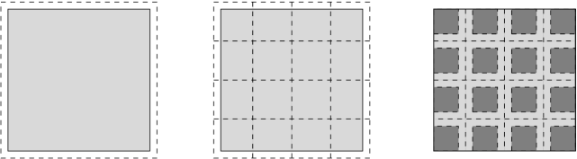
Figure 2.1. Partitioning of a square domain $\Omega$: First we expand the shaded region $\Omega$ to $\tilde{\Omega}$ (left). Next we divide $\tilde{\Omega}$ into congruent rectangles $Q_{j}$, $1\leq j\leq 16$ (middle). The flat top regions $Q_{j}^{\text{flat}}$, $1\leq j\leq 16$ are shown as the darker shaded regions (right).

2.1.2. Approximation space

The space $\mathbb{Q}_{2}$ of biquadratic polynomials will serve as the local approximation space and the global approximation space is defined to be

$$V_{h}=\{\sum_{j=1}^{N}p_{j}\Psi_{j}:\,p_{j}\in\mathbb{Q}_{2}\}.$$

Below we present an explicit basis of $V_{h}$ that will be used in our numerical computations.

On the reference interval $[-1,1]$ we have two types of quadratic polynomials:

• Lagrange interpolation polynomials $L_{i}(\xi)$ that satisfy $N_{i}(L_{j})=\delta_{ij}$ for $1\leq i,j\leq 3$, where $N_{1}(v)=v(-1)$, $N_{2}(v)=v(0)$, and $N_{3}(v)=v(1)$.

• Hermite interpolation polynomials $H_{i}(\xi)$ that satisfy $N_{i}(H_{j})=\delta_{ij}$ for $1\leq i,j\leq 3$, where $N_{1}(v)=v^{\prime}(-1)$, $N_{2}(v)=v(-1)$, and $N_{3}(v)=v(1)$.

The tensor product of different combinations of these polynomials will provide local bases on the two-dimensional rectangular patches.

Let $T_{j}:\mathbb{R}^{2}\longrightarrow\mathbb{R}^{2}$ be defined by

$$T_{j}(\xi_{1},\xi_{2})=(y_{j,1}+\xi_{1}(h_{1}/2)(1-\delta_{1}),y_{j,2}+\xi_{2}(h_{2}/2)(1-\delta_{2})).$$

Then $T_{j}$ maps the reference square $[-1,1]\times[-1,1]$ to the flat-top region $Q_{j}^{\text{flat}}$.

Depending on the location of the patch $Q_{j}$, we use different reference basis functions. There are three possibilities.

• For those patches such that $Q_{j}\cap\partial\Omega=\emptyset$, the reference basis functions are

  (2.2) $$\hat{f}_{ji}(\xi)=L_{k}(\xi_{1})L_{l}(\xi_{2}),\quad i=3(l-1)+k,\quad 1\leq k,l\leq 3.$$

• For those patches such that $Q_{j}$ intersects the boundary on only one side, say the vertical edge $x_{1}=a$ of $\Omega$, the reference basis functions are

  (2.3) $$\hat{f}_{ji}(\xi)=H_{k}(\xi_{1})L_{l}(\xi_{2}),\quad i=3(l-1)+k,\quad 1\leq k,l\leq 3.$$

  Note that in this case $T_{j}$ maps the line $\xi_{1}=-1$ to the part of $Q_{j}$ that intersects $\partial\Omega$. The cases where $Q_{j}$ intersects other sides of $\Omega$ can be treated analogously.

• For those patches such that $Q_{j}$ intersects a corner of $\Omega$, say the lower left corner $(a,c)$, the reference basis functions are

  (2.4) $$\hat{f}_{ji}(\xi)=H_{k}(\xi_{1})H_{l}(\xi_{2}),\quad i=3(l-1)+k,\quad 1\leq k,l\leq 3.$$

  Note that in this case $T_{j}$ maps the corner $(-1,-1)$ of the reference square to the lower left corner $(a,c)$ of $\Omega$. The cases where $Q_{j}$ intersects other corners of $\Omega$ can be treated analogously.

The nodal variables (or degrees of freedom) for the local approximation space are depicted in Figure 2.2, where pointwise evaluations of functions, directional derivatives, gradients and mixed second order derivatives are represented by solid dots, arrows, circles and double arrows respectively.

Figure 2.2. Reference elements described in (2.2), (2.3), and (2.4) respectively.

An explicit basis for the global approximation space $V_{h}$ is then given by

(2.5) $$\left\{\Psi_{j}\left[\hat{f}_{ji}\circ T_{j}^{-1}\right]:j=1,2,\dots,N;i=1,2,\dots,9\right\}.$$

Remark 2.2.

Since all the nodes in a rectangular patch $Q_{j}$ are located in $Q_{j}^{\text{flat}}$ where $\Psi_{k}=0$ for $k\neq j$, all the basis functions of $V_{h}$ vanish at the nodes in $Q_{j}$ except those associated with $Q_{j}$.

Figure 2.3 illustrates the degrees of freedom associated with the basis of the global approximation space for a square which is divided into $9$ square patches where $h_{1}=h_{2}=h$ and $\delta_{1}=\delta_{2}=\delta$.

Figure 2.3. A partition of a domain $\Omega$ differing only by the choice of $\delta$. The solid lines separate the different patches $Q_{j},j=1,\dots,9$. The dashed lines represent the extension of $Q_{j}$ by $\delta(h/2)$ on each side. This figure also shows the location of the degrees of freedom corresponding to $\delta=1/6$ (left) and $\delta=1/3$ (right).

Remark 2.3.

One may follow the same procedure for non-convex polygonal domains. As an example, consider an $L$-shaped domain $(-a,a)^{2}\backslash[0,a]^{2}$. One could divide the domain into rectangular patches everywhere except near the reentrant corner. Near the reentrant corner, one could construct local biquadratic polynomial basis functions in the reference $L$-shaped domain $(-1,1)^{2}\backslash[0,1]^{2}$ dual to the nodal variables

$$N_{1}(v) =v(0,0), N_{2}(v) =v(1,0), N_{3}(v) =v(0,1),$$

$$N_{4}(v) =v(-1,-1), N_{5}(v) =\frac{\partial v}{\partial\xi_{1}}(0,0), N_{6}(v) =\frac{\partial v}{\partial\xi_{1}}(0,1),$$

$$N_{7}(v) =\frac{\partial v}{\partial\xi_{2}}(0,0), N_{8}(v) =\frac{\partial v}{\partial\xi_{2}}(0,1), N_{9}(v) =\frac{\partial^{2}v}{\partial\xi_{1}\xi_{2}}(0,0),$$

as depicted in Figure 2.4.

Figure 2.4. Reference element for the $L$-shaped domain.

2.2. Interpolation Operator

First we define interpolation operators associated with the rectangular patches. Let $\zeta\in H^{2}(\mathbb{R}^{2})$.

• For a patch with the local basis given by (2.2) (cf. the reference element on the left of Figure 2.2), we define $\Pi_{j}\zeta$ to be the polynomial in $\mathbb{Q}_{2}$ such that $(\Pi_{j}\zeta)\circ T_{j}=\zeta\circ T_{j}$ at the 9 points in the set $\{(p,q):\,p,q=-1,0,1\}$.

• For a patch with the local basis given by (2.3) (cf. the reference element in the middle of Figure 2.2), we define $\Pi_{j}\zeta$ to be the polynomial in $\mathbb{Q}_{2}$ such that

  • $(\Pi_{j}\zeta)\circ T_{j}=\zeta\circ T_{j}$ at the 6 points in the set $\{(p,q):p=-1,1$ and $q=-1,0,1\}$.

  • The polynomial $({\partial[(\Pi_{j}\zeta)\circ T_{j}]}/{\partial\xi_{1}})|_{\xi_{1}=-1}$ equals the quadratic polynomial $\hat{\lambda}(\xi_{2})$, which is the $L_{2}$ projection of $({\partial(\zeta\circ T_{j})}/{\partial\xi_{1}})|_{\xi_{1}=-1}$ into the space of quadratic polynomials in the variable $\xi_{2}$.

• For a patch with the local basis given by (2.4) (cf. the reference element on the right of Figure 2.2), we define $\Pi_{j}\zeta$ to be the polynomial in $\mathbb{Q}_{2}$ such that

  • $(\Pi_{j}\zeta)\circ T_{j}=\zeta\circ T_{j}$ at the 4 points in the set $\{(p,q):p,q=\pm 1\}$.

  • $(\partial[(\Pi_{j}\zeta)\circ T_{j}]/\partial\xi_{1})|_{\xi_{1}=-1}$ equals the quadratic polynomial $\hat{\lambda}$ at $\xi_{2}=\pm 1$, where $\hat{\lambda}(\xi_{2})$ is the $L_{2}$ projection of $({\partial(\zeta\circ T_{j})}/{\partial\xi_{1}})|_{\xi_{1}=-1}$ into the space of quadratic polynomials in the variable $\xi_{2}$.

  • $(\partial[(\Pi_{j}\zeta)\circ T_{j}]/\partial\xi_{2})|_{\xi_{2}=-1}$ equals the quadratic polynomial $\hat{\mu}$ at $\xi_{1}=\pm 1$, where $\hat{\mu}(\xi_{1})$ is the $L_{2}$ projection of $({\partial(\zeta\circ T_{j})}/{\partial\xi_{2}})|_{\xi_{2}=-1}$ into the space of quadratic polynomials in the variable $\xi_{1}$.

  • The value of $(\partial^{2}[(\Pi_{j}\zeta)\circ T_{j}]/\partial\xi_{1}\partial\xi_{2})$ at $(-1,-1)$ equals $(\hat{\lambda}^{\prime}(-1)+\hat{\mu}^{\prime}(-1))/2$.

Remark 2.4.

Since $T_{j}$ maps the reference square to $Q_{j}^{\text{flat}}$, the interpolant $\Pi_{j}\zeta$ is determined by the restriction of $\zeta$ to $Q_{j}^{\text{flat}}$.

We can now define the global interpolation operator $\Pi_{h}:H^{2}(\Omega)\longrightarrow V_{h}$ by

$$\Pi_{h}\zeta=\sum_{j=1}^{N}(\Pi_{j}\zeta_{\dagger})\Psi_{j}\qquad\forall\,\zeta\in H^{2}(\Omega),$$

where $\zeta_{\dagger}\in H^{2}(\mathbb{R}^{2})$ is any extension of $\zeta$. The interpolant $\Pi_{h}$ is independent of the choice of $\zeta_{\dagger}$ by Remark 2.4. Moreover, by construction we have

(2.6) $$\Pi_{h}(H^{2}_{0}(\Omega))=V_{h}\cap H^{2}_{0}(\Omega).$$

Let $\tilde{Q}_{j}$ be the rectangle centered at $y_{j}$ with width $h_{1}(1+\delta_{1})=h_{1}+2\gamma_{1}$ and height $h_{2}(1+\delta_{2})=h_{2}+2\gamma_{2}$. Let $h=\max(h_{1},h_{2})$. Since $\Pi_{j}P=P$ for any $P\in\mathbb{Q}_{2}$, the estimate

(2.7) $$\sum_{m=0}^{2}h^{m}|\zeta-\Pi_{j}\zeta|_{H^{m}(\tilde{Q}_{j}\cap\Omega)}\leq Ch^{2+\alpha}|\zeta|_{H^{2+\alpha}(\tilde{Q}_{j}\cap\Omega)}$$

follows from the Bramble-Hilbert lemma [7, 18] and scaling. From here on we use $C$ to denote a generic positive constant that is independent of the mesh size $h$.

Combining the local interpolation error estimate (2.7) and the estimates for the partition of unity functions $\Psi_{j}$ in [32], we immediately have (cf. [29, 32]) the following error estimates for the global interpolation operator $\Pi_{h}$:

(2.8) $$\sum_{m=0}^{2}h^{m}|\zeta-\Pi_{h}\zeta|_{H^{m}(\Omega)}\leq Ch^{2+\alpha}|\zeta|_{H^{2+\alpha}(\Omega)}.$$

Remark 2.5.

Classical rectangular $C^{1}$ finite element methods would require a local approximation space that is at least bi-cubic [6]. Of course we can also use bi-cubic polynomials as the local approximation space in our GFEM (cf. [17, 31] and Example 1 in Section 4).

2.3. The Discrete Obstacle Problem

Let $\mathcal{V}_{h}$ be the set of the nodes in the rectangular patches corresponding to the degrees of freedom involving pointwise evaluation of the local basis functions. (Such nodes are represented by solid dots in Figure 2.3 and Figure 2.4.) The GFEM for the model problem is to find $u_{h}\in K_{h}$ such that

(2.9) $$u_{h}=\mathop{\rm argmin}_{v\in K_{h}}G(v),$$

where the quadratic functional $G$ is defined by (1.4)–(1.5) and

(2.10) $$K_{h} = \{v\in V_{h}:v-\Pi_{h}g\in H^{2}_{0}(\Omega),\,\psi_{1}(p)\leq v(p)\leq\psi_{2}(p)\quad\forall p\in\mathcal{V}_{h}\}.$$

Remark 2.6.

Approximation of the essential boundary conditions $u=g$ and ${\partial u}/{\partial n}={\partial g}/{\partial n}$ are both included in the definition of $K_{h}$. Moreover $K_{h}$ is nonempty because $\Pi_{h}K\subset K_{h}$ by (1.3) and (2.6).

Remark 2.7.

In view of Remark 2.2 and the defining properties of the polynomials $L_{i}$ and $H_{i}$, the constraints defining $K_{h}$ are box constraints with respect to the basis of $V_{h}$ defined in (2.5).

It follows from the standard theory that the discrete obstacle problem (2.9) has a unique solution characterized by the discrete variational inequality

(2.11) $$a(u_{h},v-u_{h})\geq(f,v-u_{h})\quad\forall v\in K_{h}.$$

3. Convergence Analysis

We begin with some preliminary estimates in Section 3.1 and introduce an auxiliary obstacle problem in Section 3.2 that connects the continuous problem (1.2) and the discrete problem (2.9). The main result is derived in Section 3.3.

3.1. Preliminary Estimates

In view of (2.8), it suffices to find an optimal estimate for $|\Pi_{h}u-u_{h}|_{H^{2}(\Omega)}$. Using the discrete variational inequality (2.11), we have

$$|\Pi_{h}u-u_{h}|_{H^{2}(\Omega)}^{2} =a(\Pi_{h}u-u,\Pi_{h}u-u_{h})+a(u-u_{h},\Pi_{h}u-u_{h})$$

$$\leq|\Pi_{h}u-u|_{H^{2}(\Omega)}|\Pi_{h}u-u_{h}|_{H^{2}(\Omega)}+a(u,\Pi_{h}u-u_{h})-(f,\Pi_{h}u-u_{h})$$

$$\leq\frac{1}{2}|\Pi_{h}u-u|_{H^{2}(\Omega)}^{2}+\frac{1}{2}|\Pi_{h}u-u_{h}|_{H^{2}(\Omega)}^{2}+a(u,\Pi_{h}u-u_{h})-(f,\Pi_{h}u-u_{h}),$$

which implies

(3.1) $$|\Pi_{h}u-u_{h}|_{H^{2}(\Omega)}^{2}\leq|\Pi_{h}u-u|_{H^{2}(\Omega)}^{2}+2\big{[}a(u,\Pi_{h}u-u_{h})-(f,\Pi_{h}u-u_{h})\big{]}.$$

We can therefore complete the error analysis by finding an optimal estimate for the expression $a(u,\Pi_{h}u-u_{h})-(f,\Pi_{h}u-u_{h})$.

The following result is useful for the error analysis in Section 3.3.

Lemma 3.1.

There exists a positive constant $C$ independent of $h$ such that

(3.2) $$|a(\phi,\zeta-\Pi_{h}\zeta)|\leq Ch^{2\alpha}\|\phi\|_{H^{2+\alpha}(\Omega)}\|\zeta\|_{H^{2+\alpha}(\Omega)}$$

for all $\phi\in H^{2+\alpha}(\Omega)$ and $\zeta\in H^{2+\alpha}(\Omega)\cap H^{2}_{0}(\Omega)$.

Proof.

Let $\zeta\in H^{2+\alpha}(\Omega)\cap H^{2}_{0}(\Omega)$ be arbitrary. On the one hand we have an obvious estimate

(3.3) $$|a(\phi,\zeta-\Pi_{h}\zeta)| \leq|\phi|_{H^{2}(\Omega)}|\zeta-\Pi_{h}\zeta|_{H^{2}(\Omega)}$$

$$\leq Ch^{\alpha}|\phi|_{H^{2}(\Omega)}|\zeta|_{H^{2+\alpha}(\Omega)}\qquad\forall\,\phi\in H^{2}(\Omega)$$

that follows from (2.8). On the other hand, we have another estimate

$$|a(\phi,\zeta-\Pi_{h}\zeta)| =\Big{|}\int_{\Omega}(\nabla\cdot\nabla^{2}\phi)\cdot\nabla(\zeta-\Pi_{h}\zeta)\,dx\Big{|}$$

(3.4) $$\leq C|\phi|_{H^{3}(\Omega)}|\zeta-\Pi_{h}\zeta|_{H^{1}(\Omega)}$$

$$\leq Ch^{1+\alpha}|\phi|_{H^{3}(\Omega)}|\zeta|_{H^{2+\alpha}(\Omega)}\qquad\forall\,\phi\in H^{3}(\Omega)$$

that follows from (2.6), (2.8) and integration by parts.

The estimate (3.2) follows from (3.3), (3.1) and interpolation between Sobolev spaces [1, 33]. ∎

3.2. An Auxiliary Obstacle Problem

We can connect the continuous obstacle problem (1.2) and the discrete obstacle problem (2.9) through an intermediate obstacle problem: Find $\tilde{u}_{h}\in\tilde{K}_{h}$ such that

(3.5) $$\tilde{u}_{h}=\mathop{\rm argmin}_{v\in\tilde{K}_{h}}G(v)$$

where

(3.6) $$\tilde{K}_{h}=\{v\in H^{2}(\Omega):v-g\in H^{2}_{0}(\Omega),\psi_{1}(p)\leq v(p)\leq\psi_{2}(p)\quad\forall p\in\mathcal{V}_{h}\}.$$

Note that $\tilde{K}_{h}$ is a closed convex subset of $H^{2}(\Omega)$ and $K\subset\tilde{K}_{h}.$ The unique solution of (3.5) is characterized by the variational inequality:

(3.7) $$a(\tilde{u}_{h},v-\tilde{u}_{h})\geq(f,v-\tilde{u}_{h})\quad\forall v\in\tilde{K}_{h}.$$

The connection between (1.2) and (3.5) is given by the following properties of $\tilde{u}_{h}$ from [10, 9]:

(3.8) $$|u-\tilde{u}_{h}|_{H^{2}(\Omega)}\leq Ch,$$

and there exists $h_{0}>0$ such that

(3.9) $$\hat{u}_{h}=\tilde{u}_{h}+\delta_{h,1}\phi_{1}-\delta_{h,2}\phi_{2}\in K\quad\forall\,h\leq h_{0},$$

where $\phi_{1}$ and $\phi_{2}$ are $C^{\infty}$ functions with compact supports in $\Omega$ such that $\phi_{i}=1$ on the coincidence set $\{x\in\Omega:\,u(x)=\psi_{i}(x)\}$, and the positive numbers $\delta_{h,1}$ and $\delta_{h,2}$ satisfy

(3.10) $$\delta_{h,i}\leq Ch^{2}.$$

Note that $v-\Pi_{h}g\in H^{2}_{0}(\Omega)$ for all $v\in K_{h}$ (cf. (2.10)) and hence, by (3.6),

(3.11) $$v+(g-\Pi_{h}g)\in{\tilde{K}}_{h}\qquad\forall\,v\in K_{h}.$$

3.3. Error Estimates for the Generalized Finite Element Method

We now complete the error analysis of the generalized finite element method by deriving an optimal estimate for the expression $a(u,\Pi_{h}-u_{h})-(f,\Pi_{h}u-u_{h})$. To simplify the presentation, we introduce the transitive relation $A\hskip 4.0pt\raise 1.0pt\hbox{$\leq$}\lower 4.0pt\hbox{.}\hskip 6.0ptB$ defined by

$$A\hskip 4.0pt\raise 1.0pt\hbox{$\leq$}\lower 4.0pt\hbox{.}\hskip 6.0ptB\Leftrightarrow A-B\leq C(h^{2\alpha}+h^{\alpha}|\Pi_{h}u-u_{h}|_{H^{2}(\Omega)}).$$

Since

$$a(u,\Pi_{h}u-u_{h})=a(u-{\tilde{u}}_{h},\Pi_{h}u-u_{h})+a({\tilde{u}}_{h},\Pi_{h}u-u_{h})$$

and

$$a(u-{\tilde{u}}_{h},\Pi_{h}u-u_{h})\leq|u-{\tilde{u}}_{h}|_{H^{2}(\Omega)}|\Pi_{h}u-u_{h}|_{H^{2}(\Omega)}\leq Ch|\Pi_{h}u-u_{h}|_{H^{2}(\Omega)}$$

by the estimate (3.8), we have

(3.12) $$a(u,\Pi_{h}u-u_{h})-(f,\Pi_{h}u-u_{h})\hskip 4.0pt\raise 1.0pt\hbox{$\leq$}\lower 4.0pt\hbox{.}\hskip 6.0pta({\tilde{u}}_{h},\Pi_{h}u-u_{h})-(f,\Pi_{h}u-u_{h}).$$

In view of (3.11), we can use the auxiliary variational inequality (3.7) to obtain

$$a({\tilde{u}}_{h},\Pi_{h}u-u_{h}) =a({\tilde{u}}_{h},{\tilde{u}}_{h}-u_{h}-(g-\Pi_{h}g))+a({\tilde{u}}_{h},\Pi_{h}u-{\tilde{u}}_{h}+(g-\Pi_{h}g))$$

$$\leq(f,{\tilde{u}}_{h}-u_{h}-(g-\Pi_{h}g))+a({\tilde{u}}_{h},\Pi_{h}u-{\tilde{u}}_{h}+(g-\Pi_{h}g)),$$

which together with (3.12) implies

(3.13) $$a(u,\Pi_{h}u-u_{h})-(f,\Pi_{h}u-u_{h})\hskip 4.0pt\raise 1.0pt\hbox{$\leq$}\lower 4.0pt\hbox{.}\hskip 6.0pt$$

$$\hskip 50.0pta({\tilde{u}}_{h},\Pi_{h}u-{\tilde{u}}_{h}+(g-\Pi_{h}g))-(f,u-{\tilde{u}}_{h})-(f,(\Pi_{h}u-u)+(g-\Pi_{h}g)).$$

We can rewrite the first term on the right-hand side of (3.13) as

$$a({\tilde{u}}_{h},\Pi_{h}u-{\tilde{u}}_{h}+(g-\Pi_{h}g)) =a({\tilde{u}}_{h}-u,\Pi_{h}u-{\tilde{u}}_{h}+(g-\Pi_{h}g))+a(u,\Pi_{h}(u-g)-(u-g))$$

$$\hskip 30.0pt+a(u,u-{\tilde{u}}_{h}).$$

Observe that

$$a({\tilde{u}}_{h}-u,\Pi_{h}u-{\tilde{u}}_{h}+(g-\Pi_{h}g))=a({\tilde{u}}_{h}-u,(\Pi_{h}u-u)+(u-{\tilde{u}}_{h})+(g-\Pi_{h}g))$$

$$\hskip 70.0pt\leq|{\tilde{u}}_{h}-u|_{H^{2}(\Omega)}\big{(}|\Pi_{h}u-u|_{H^{2}(\Omega)}+|u-{\tilde{u}}_{h}|_{H^{2}(\Omega)}+|g-\Pi_{h}g|_{H^{2}(\Omega)}\big{)}$$

$$\hskip 70.0pt\leq Ch^{1+\alpha}$$

by (2.8) and (3.8), and

$$a(u,\Pi_{h}(u-g)-(u-g))\leq Ch^{2\alpha}$$

by Lemma 3.1. Moreover we have, by (2.8),

$$-(f,(\Pi_{h}u-u)+(g-\Pi_{h}g))\leq\|f\|_{L_{2}(\Omega)}\big{(}\|\Pi_{h}u-u\|_{L_{2}(\Omega)}+\|g-\Pi_{h}g\|_{L_{2}(\Omega)}\big{)}\leq Ch^{2+\alpha}.$$

Combining these relations and (3.13), we arrive at the estimate

(3.14) $$a(u,\Pi_{h}u-u_{h})-(f,\Pi_{h}u-u_{h}).\hskip 4.0pt\raise 1.0pt\hbox{$\leq$}\lower 4.0pt\hbox{.}\hskip 6.0pta(u,u-{\tilde{u}}_{h})-(f,u-{\tilde{u}}_{h}).$$

According to (1.6), (3.9) and (3.10), we have

$$a(u,u-{\tilde{u}}_{h})-(f,u-{\tilde{u}}_{h})$$

$$\hskip 30.0pt=a(u,u-\hat{u}_{h})-(f,u-\hat{u}_{h})+\delta_{h,1}[a(u,\phi_{1})-(f,\phi_{1})]-\delta_{h,2}[a(u,\phi_{2})-(f,\phi_{2})]$$

$$\hskip 30.0pt\leq Ch^{2},$$

and hence (3.14) leads to the estimate

$$a(u,\Pi_{h}u-u_{h})-(f,\Pi_{h}u-u_{h})\hskip 4.0pt\raise 1.0pt\hbox{$\leq$}\lower 4.0pt\hbox{.}\hskip 6.0pt0,$$

which means

(3.15) $$a(u,\Pi_{h}u-u_{h})-(f,\Pi_{h}u-u_{h})\leq C(h^{2\alpha}+h^{\alpha}|\Pi_{h}u-u_{h}|_{H^{2}(\Omega)}).$$

Theorem 3.2.

There exists a positive constant $C$ independent of $h$ such that

$$|u-u_{h}|_{H^{2}(\Omega)}\leq Ch^{\alpha}.$$

Proof.

It follows from (2.8), (3.1), (3.15) and the arithmetic and geometric means inequality that

$$|\Pi_{h}u-u_{h}|_{H^{2}(\Omega)}^{2}\leq C(h^{2\alpha}+h^{\alpha}|\Pi_{h}u-u_{h}|_{H^{2}(\Omega)})\leq Ch^{2\alpha}+\frac{1}{2}|\Pi_{h}u-u_{h}|_{H^{2}(\Omega)}^{2},$$

which implies

(3.16) $$|\Pi_{h}u-u_{h}|_{H^{2}(\Omega)}\leq Ch^{\alpha}.$$

The theorem follows from (2.8), (3.16) and the triangle inequality. ∎

Since $H^{2}(\Omega)$ is embedded in $C(\bar{\Omega})$ by the Sobolev embedding theorem [1, 33], the following corollary is immediate. But numerical results in Section 4 indicate that the convergence rate in the $L_{\infty}(\Omega)$ norm should be higher than the convergence rate in the $H^{2}(\Omega)$ norm.

Corollary 3.3.

There exists a positive constant $C$ independent of $h$ such that

(3.17) $$|u-u_{h}|_{L_{\infty}(\Omega)}\leq Ch^{\alpha}.$$

Remark 3.4.

Under additional assumptions [12, 30] on the exact coincidence sets (resp. free boundaries), the error estimate (3.17) implies the convergence of the discrete coincidence sets (resp. free boundaries) to the exact coincidence sets (resp. free boundaries). Details can be found in [9].

4. Numerical Results

We present numerical results for several one-obstacle problems to demonstrate the performance of the GFEM. The obstacle function from below will be denoted by $\psi.$ The first four examples are from [9]. The discrete obstacle problems are solved by a primal dual active set strategy from [4, 25].

Example 1. Here we apply the GFEM to a problem with a known exact solution to validate the numerical results. We begin with the plate obstacle problem on the disc $\{x:|x|<2\}$ with $f=0,\psi(x)=1-|x|^{2}$ and homogeneous Dirichlet boundary conditions. This problem is rotationally invariant and can be solved exactly. The exact solution is

$$u(x)=\begin{cases}C_{1}|x|^{2}\ln|x|+C_{2}|x|^{2}+C_{3}\ln|x|+C_{4},&r_{0}<|x|<2\\ 1-|x|^{2},&|x|\leq r_{0}\end{cases}$$

where $r_{0}\approx 0.18134452,C_{1}\approx 0.52504063,C_{2}\approx-0.62860904,C_{3}\approx 0.01726640,$ and $C_{4}\approx 1.04674630.$ We then consider the obstacle problem on $\Omega=(-0.5,0.5)^{2}$ whose exact solution is the restriction of $u$ to $\Omega.$ For this problem $f=0,\psi(x)=1-|x|^{2}$ and the (non-homogeneous) Dirichlet boundary data are determined by $u.$

We partition $\Omega$ following the procedure described in Section 2.1 and define $j$ to be the level where there are $2^{j}$ equal subdivisions in each direction. We solve the discrete obstacle problem on each level $j$ with $\delta=1/3$ so that the mesh parameter $h_{j}=(2^{j}-1/3)^{-1}$.

We denote the energy norm on the $j$-th level by $\|\cdot\|_{j}$. Let $u_{j}$ be the numerical solution of the $j$-th level discrete obstacle problem and $e_{j}=\Pi_{j}u-u_{j}$ where $\Pi_{j}$ is the interpolation operator on the $j-$th level. We evaluate the error $\|e_{j}\|_{j}$ in the energy norm, and the error $\|e_{j}\|_{\infty}$ in the $\ell_{\infty}$ norm, and compute the rates of convergence in these norms by

$$\beta_{h}=\ln(\|e_{j/2}\|_{j/2}/\|e_{j}\|_{j})/\ln(h_{j/2}/h_{j})\quad\text{ and }\quad\beta_{\infty}=\ln(\|e_{j/2}\|_{\infty}/\|e_{j}\|_{\infty})/\ln(h_{j/2}/h_{j}).$$

The numerical results are presented in Table 4.1. It is observed that the magnitude of the error in energy norm is $O(h)$.

$j$	$\|e_{j}\|_{j}/\|u_{8}\|_{8}$	$\beta_{h}$	$\|e_{j}\|_{\infty}$	$\beta_{\infty}$
1	0.0000 $\times 10^{-0}$		0.0000 $\times 10^{-0}$
2	1.2365 $\times 10^{-1}$		8.8312 $\times 10^{-4}$
3	6.3226 $\times 10^{-2}$	0.9094	6.0088 $\times 10^{-4}$	0.5221
4	2.5977 $\times 10^{-2}$	1.2447	8.8401 $\times 10^{-5}$	2.6817
5	1.2159 $\times 10^{-2}$	1.0787	2.4443 $\times 10^{-5}$	1.8267
6	5.9045 $\times 10^{-3}$	1.0343	6.7946 $\times 10^{-6}$	1.8331
7	2.9125 $\times 10^{-3}$	1.0157	1.4775 $\times 10^{-6}$	2.1929
8	1.4396 $\times 10^{-3}$	1.0147	8.8608 $\times 10^{-7}$	0.7363

Table 4.1. Energy norm and $\ell_{\infty}$ norm errors for Example 1.

The exact coincidence set $I$ for this example is the disc centered at $(0,0)$ with radius $r_{0}$. Let $\mathcal{V}_{j}$ be the set of nodes on the $j$-th level corresponding to degrees of freedom involving pointwise evaluation of local basis functions in the interior of $\Omega$. Then we define the discrete coincidence set $I_{j}$ by

$$I_{j}=\{p\in\mathcal{V}_{j}:u_{j}(p)-\psi(p)\leq\|e_{j}\|_{\infty}\}.$$

The discrete coincidence sets $I_{7}$ and $I_{8}$ are displayed in Figure 4.1, where the radius of the circle in black is $r_{0}$. The convergence of the discrete coincidence sets is observed.

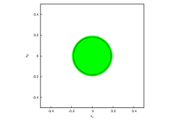
Figure 4.1. Discrete coincidence set for Example 1 for level 7 (left) and level 8 (right).

One of the advantages of the GFEM is that the local approximation space can be easily adjusted. In Table 4.2 we report the numerical results for the same problem but with $\mathbb{Q}_{3}$ as the local approximation space. An $O(h^{1.5})$ energy error is observed, which is due to the fact that the exact solution $u$ is piecewise smooth.

$j$	$\|e_{j}\|_{j}/\|u_{8}\|_{8}$	$\beta_{h}$	$\|e_{j}\|_{\infty}$	$\beta_{\infty}$
1	1.4199 $\times 10^{-2}$		1.0561 $\times 10^{-4}$
2	6.1489 $\times 10^{-2}$	-1.8589	7.6281 $\times 10^{-4}$	-2.5078
3	1.8374 $\times 10^{-2}$	1.6377	9.4507 $\times 10^{-5}$	2.8313
4	5.8004 $\times 10^{-3}$	1.6134	1.4396 $\times 10^{-5}$	2.6330
5	2.3728 $\times 10^{-3}$	1.2702	4.7114 $\times 10^{-6}$	1.5872
6	8.3768 $\times 10^{-4}$	1.4908	4.1685 $\times 10^{-7}$	3.4723
7	2.7675 $\times 10^{-4}$	1.5918	3.7129 $\times 10^{-6}$	-3.1431

Table 4.2. Energy norm and $\ell_{\infty}$ norm errors for Example 1 with $\mathbb{Q}_{3}$ as local approximation space.

Remark 4.1.

Note that the $\ell_{\infty}$ norm errors fluctuate. This is likely due to the fact that the primal dual active set strategy is based on stopping conditions that are unrelated to the $\ell_{\infty}$ norm.

Example 2. In this example we take $\Omega=(-0.5,0.5)^{2},f=g=0$ and $\psi(x)=1-5|x|^{2}+|x|^{4}.$ We solve the discrete obstacle problems using the same PU functions as in Example 1.

Since the exact solution is not known, we take $\tilde{e}_{j}=\Pi_{j}u_{j-1}-u_{j}$ and compute the rates of convergence $\tilde{\beta}_{h}$ and $\tilde{\beta}_{\infty}$ by

$$\tilde{\beta}_{h}=\ln(\|\tilde{e}_{j/2}\|_{j/2}/\|\tilde{e}_{j}\|_{j})/\ln(h_{j/2}/h_{j})\quad\text{ and }\quad\tilde{\beta}_{\infty}=\ln(\|\tilde{e}_{j/2}\|_{\infty}/\|\tilde{e}_{j}\|_{\infty})/\ln(h_{j/2}/h_{j}).$$

The results are presented in Table 4.3.

$j$	$\|\tilde{e}_{j}\|_{j}/\|u_{8}\|_{8}$	$\tilde{\beta}_{h}$	$\|\tilde{e}_{j}\|_{\infty}$	$\tilde{\beta}_{\infty}$
1	2.9288 $\times 10^{-0}$		9.0040 x $\times 10^{-1}$
2	5.9820 $\times 10^{-0}$	-0.9058	5.3416 x $\times 10^{-1}$	0.6622
3	1.2402 $\times 10^{-0}$	2.1333	5.2357 $\times 10^{-1}$	0.0271
4	6.5242 $\times 10^{-1}$	0.8988	2.5914 $\times 10^{-2}$	4.2061
5	1.8496 $\times 10^{-1}$	1.7913	1.7757 $\times 10^{-3}$	3.8091
6	8.9273 $\times 10^{-2}$	1.0430	4.4337 $\times 10^{-4}$	1.9867
7	4.4296 $\times 10^{-2}$	1.0072	1.1284 $\times 10^{-4}$	1.9667
8	2.2154 $\times 10^{-2}$	0.9977	3.7776 $\times 10^{-5}$	1.5758

Table 4.3. Energy norm and $\ell_{\infty}$ norm errors for Example 2.

Since $\Delta^{2}\psi-f>0$ in this example, the non-coincidence set is known to be connected [15]. This is confirmed by the discrete coincidence sets $I_{7}$ and $I_{8}$ displayed in Figure 4.2. Note that the discrete coincidence sets have the correct symmetries: rotations by right angles and reflections across coordinates axes.

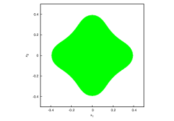
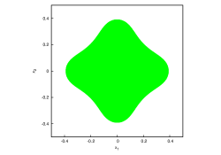
Figure 4.2. Discrete coincidence set for Example 2 for level 7 (left) and level 8 (right).

Example 3. In this example we take $\Omega=(-0.5,0.5)^{2}$, $f=g=0$ and $\psi(x)=1-5|x|^{2}-|x|^{4}$. We solve the discrete obstacle problems using the same PU functions as in Example 1. Numerical results are tabulated in Table 4.4.

$j$	$\|\tilde{e}_{j}\|_{j}/\|u_{8}\|_{8}$	$\tilde{\beta}_{h}$	$\|\tilde{e}_{j}\|_{\infty}$	$\tilde{\beta}_{\infty}$
1	3.0796 $\times 10^{-0}$		8.9960 $\times 10^{-1}$
2	6.2833 $\times 10^{-0}$	-0.9044	4.8507 $\times 10^{-1}$	0.7834
3	1.0279 $\times 10^{-0}$	2.4544	4.3181 $\times 10^{-1}$	0.1576
4	2.9125 $\times 10^{-1}$	1.7646	1.9025 $\times 10^{-2}$	4.3689
5	1.4890 $\times 10^{-1}$	0.9533	1.6296 $\times 10^{-3}$	3.4920
6	7.1583 $\times 10^{-2}$	1.0487	4.8682 $\times 10^{-4}$	1.7300
7	3.6108 $\times 10^{-2}$	0.9836	1.3055 $\times 10^{-4}$	1.8916
8	1.8072 $\times 10^{-2}$	0.9966	3.1174 $\times 10^{-5}$	2.0623

Table 4.4. Energy norm and $\ell_{\infty}$ norm errors for Example 3.

The set-up for Example 3 is very similar to that of Example 2, except that now $\Delta^{2}\psi-f<0$ and hence the interior of the coincidence set must be empty, otherwise the complementarity form of the variational inequality would be violated. This is confirmed by the discrete coincidence sets in Figure 4.3, which also possess the correct symmetries.

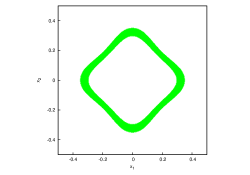
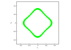
Figure 4.3. Discrete coincidence set for Example 3 for level 7 (left) and level 8 (right).

Example 4. In this example we take $\Omega$ to be the $L$-shaped domain $(-0.5,0.5)^{2}\backslash[0,0.5]^{2}$, $f=g=0$ and $\psi(x)=1-\left[\frac{(x_{1}+0.25)^{2}}{0.2^{2}}+\frac{x_{2}^{2}}{0.35^{2}}\right].$ We solve the discrete obstacle problems using a similar partition as described in Section 2.1. For this example, $j$ is chosen so that it is the level where there are $2^{j}+1$ subdivisions in each direction, making $h_{j}=(2^{j}+1-1/3)^{-1}.$ This allows us to insert an $L$-shaped element in the vicinity of the reentrant corner as described in Remark 2.3.

From the numerical results in Table 4.5 we observe that $\tilde{\beta}_{h}$ is approaching $\mathcal{O}(h^{\alpha})$ where $\alpha=0.544$ is the index of elliptic regularity for the $L$-shaped domain, as predicted by Theorem 3.2.

$j$	$\|\tilde{e}_{j}\|_{j}/\|u_{8}\|_{8}$	$\tilde{\beta}_{h}$	$\|\tilde{e}_{j}\|_{\infty}$	$\tilde{\beta}_{\infty}$
1	4.4737 $\times 10^{-0}$		1.0000 $\times 10^{-0}$
2	6.9545 $\times 10^{-0}$	-0.7884	5.9996 $\times 10^{-1}$	0.9129
3	2.9079 $\times 10^{-0}$	1.4086	3.2598 $\times 10^{-1}$	0.9854
4	1.8562 $\times 10^{-0}$	0.6864	1.3853 $\times 10^{-1}$	1.3086
5	6.9086 $\times 10^{-1}$	1.4687	4.0400 $\times 10^{-2}$	1.8312
6	2.8930 $\times 10^{-1}$	1.2747	2.9381 $\times 10^{-2}$	0.4664
7	1.6919 $\times 10^{-1}$	0.7797	1.4457 $\times 10^{-2}$	1.0308
8	1.0582 $\times 10^{-1}$	0.6796	6.9259 $\times 10^{-3}$	1.0657

Table 4.5. Energy norm and $\ell_{\infty}$ norm errors for Example 4.

Since $\Delta^{2}\psi-f=0$ for this example, the non-coincidence set is connected [15], which is confirmed by Figure 4.4.

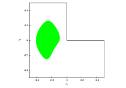
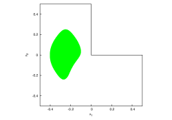
Figure 4.4. Discrete coincidence set for Example 4 for level 7 (left) and level 8 (right).

Example 5. In this example we take $\Omega$ to be the pentagon $\{x\in(-0.5,0.5)^{2}:x_{1}+x_{2}<0.5\}$. We take $f=g=0$ and $\psi(x)=1-9|x|^{2}.$ We solve the discrete obstacle problems using a similar partition as described in Section 2.1. For this example, $j$ is chosen so that it is the level where there are $2^{j}+1$ subdivisions in each direction, making $h_{j}=(2^{j}+1-1/3)^{-1}.$ This allows us to insert different types of elements near the obtuse vertices of $\Omega$, see Figure 4.5 and Figure 4.6. The numerical results are reported in Table 4.6.

Figure 4.5. Reference elements for the pentagonal domain.

Figure 4.6. A partition of the pentagonal domain $\Omega$ for levels $j=1$ (left) and $j=2$ (right). The solid lines separate the different patches $Q_{j},j=1,\dots,9$ (left) and $Q_{j},j=1,\ldots,25$ (right). The dashed lines represent the extension of $Q_{j}$ by $\delta(h/2)$ on each side. This figure also shows the locations of the degrees of freedom.

$j$	$\|\tilde{e}_{j}\|_{j}/\|u_{8}\|_{8}$	$\tilde{\beta}_{h}$	$\|\tilde{e}_{j}\|_{\infty}$	$\tilde{\beta}_{\infty}$
1	5.1600 $\times 10^{-0}$		1.0628 $\times 10^{-0}$
2	1.0383 $\times 10^{+1}$	-1.2495	1.1233 $\times 10^{-0}$	0.0989
3	4.8834 $\times 10^{-0}$	1.2185	4.6694 $\times 10^{-1}$	1.4181
4	3.6378 $\times 10^{-0}$	0.4503	2.5049 $\times 10^{-1}$	0.9524
5	1.5514 $\times 10^{-0}$	1.2664	2.7118 $\times 10^{-2}$	3.3037
6	6.5449 $\times 10^{-1}$	1.2639	4.5364 $\times 10^{-3}$	2.6183
7	2.8868 $\times 10^{-1}$	1.1898	9.0815 $\times 10^{-4}$	2.3380
8	1.3864 $\times 10^{-1}$	1.0621	1.7631 $\times 10^{-4}$	2.3737

Table 4.6. Energy norm and $\ell_{\infty}$ norm errors for Example 5.

Since $\Delta^{2}\psi-f=0$ in this example, the non-coincidence set is connected [15], which is confirmed by Figure 4.7, where the discrete coincidence sets also display the correct reflection symmetry.

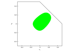
Figure 4.7. Discrete coincidence set for Example 5 for level 7 (left) and level 8 (right).

References

- [1] R.A. Adams and J.J.F. Fournier. Sobolev Spaces Second Edition. Academic Press, Amsterdam, 2003.
- [2] I. Babuška and U. Banerjee. Stable generalized finite element method (SGFEM). Comput. Methods Appl. Mech. Engrg., 201/204:91–111, 2012.
- [3] I. Babuška, U. Banerjee, and J.E. Osborn. Survey of meshless and generalized finite element methods: a unified approach. Acta Numer., 12:1–125, 2003.
- [4] M. Bergounioux, K. Ito, and K. Kunisch. Primal-dual strategy for constrained optimal control problems. SIAM J. Control Optim., 37:1176–1194 (electronic), 1999.
- [5] H. Blum and R. Rannacher. On the boundary value problem of the biharmonic operator on domains with angular corners. Math. Methods Appl. Sci., 2:556–581, 1980.
- [6] F.K. Bogner, R.L. Fox, and L.A. Schmit. The generation of interelement compatible stiffness and mass matrices by the use of interpolation formulas. In Proceedings Conference on Matrix Methods in Structural Mechanics, pages 397–444. Wright Patterson A.F.B., Dayton, OH, 1965.
- [7] J.H. Bramble and S.R. Hilbert. Estimation of linear functionals on Sobolev spaces with applications to Fourier transforms and spline interpolation. SIAM J. Numer. Anal., 7:113–124, 1970.
- [8] S.C. Brenner, L.-Y. Sung, H. Zhang, and Y. Zhang. A Morley finite element method for the displacement obstacle problem of clamped Kirchhoff plates. preprint, 2011.
- [9] S.C. Brenner, L.-Y. Sung, H. Zhang, and Y. Zhang. A quadratic interior penalty method for the displacement obstacle problem of clamped Kirchhoff plates. SIAM J. Numer. Anal., (to appear).
- [10] S.C. Brenner, L.-Y. Sung, and Y. Zhang. Finite element methods for the displacement obstacle problem of clamped plates. Math. Comp., 81:1247–1262, 2012.
- [11] H. R. Brezis and G. Stampacchia. Sur la régularité de la solution d’inéquations elliptiques. Bull. Soc. Math. France, 96:153–180, 1968.
- [12] F. Brezzi and L.A. Caffarelli. Convergence of the discrete free boundaries for finite element approximations. RAIRO Anal. Numér., 17:385–395, 1983.
- [13] F. Brezzi, W. Hager, and P.-A. Raviart. Error estimates for the finite element solution of variational inequalities. Numer. Math., 28:431–443, 1977.
- [14] F. Brezzi, W. Hager, and P.-A. Raviart. Error estimates for the finite element solution of variational inequalities. II. Mixed methods. Numer. Math., 31:1–16, 1978/79.
- [15] L.A. Caffarelli and A. Friedman. The obstacle problem for the biharmonic operator. Ann. Scuola Norm. Sup. Pisa Cl. Sci. (4), 6:151–184, 1979.
- [16] M. Dauge. Elliptic Boundary Value Problems on Corner Domains, Lecture Notes in Mathematics 1341. Springer-Verlag, Berlin-Heidelberg, 1988.
- [17] C.B. Davis. Meshless Boundary Particle Methods for Boundary Integral Equations and Meshfree Particle Methods for Plates. PhD thesis, University of North Carolina at Charlotte, 2011.
- [18] T. Dupont and R. Scott. Polynomial approximation of functions in Sobolev spaces. Math. Comp., 34:441–463, 1980.
- [19] R.S. Falk. Error estimates for the approximation of a class of variational inequalities. Math. Comp., 28:963 –971, 1974.
- [20] J. Frehse. Zum Differenzierbarkeitsproblem bei Variationsungleichungen höherer Ordnung. Abh. Math. Sem. Univ. Hamburg, 36:140–149, 1971.
- [21] J. Frehse. On the regularity of the solution of the biharmonic variational inequality. Manuscripta Math., 9:91–103, 1973.
- [22] A. Friedman. Variational Principles and Free-Boundary Problems. Robert E. Krieger Publishing Co. Inc., Malabar, FL, second edition, 1988.
- [23] R. Glowinski, J.-L. Lions, and R. Trémolières. Numerical Analysis of Variational Inequalities. North-Holland Publishing Co., Amsterdam, 1981.
- [24] P. Grisvard. Elliptic Problems in Non Smooth Domains. Pitman, Boston, 1985.
- [25] M. Hintermüller, K. Ito, and K. Kunisch. The primal-dual active set strategy as a semismooth Newton method. SIAM J. Optim., 13:865–888 (2003), 2002.
- [26] D. Kinderlehrer and G. Stampacchia. An Introduction to Variational Inequalities and Their Applications. SIAM, Philadelphia, 2000.
- [27] V.A. Kozlov, V.G. Maz’ya, and J. Rossmann. Spectral Problems Associated with Corner Singularities of Solutions to Elliptic Problems. AMS, Providence, 2001.
- [28] J.-L. Lions and G. Stampacchia. Variational inequalities. Comm. Pure Appl. Math., 20:493–519, 1967.
- [29] J.M. Melenk and I. Babuška. The partition of unity finite element method: basic theory and applications. Comput. Methods Appl. Mech. Engrg., 139:289–314, 1996.
- [30] R.H. Nochetto. A note on the approximation of free boundaries by finite element methods. RAIRO Modél. Math. Anal. Numér., 20:355–368, 1986.
- [31] H.-S. Oh, C. Davis, and J.W. Jeong. Meshfree particle methods for thin plates. Comput. Methods Appl. Mech. Engrg., 209:156–171, 2012.
- [32] H.-S. Oh, J.G. Kim, and W.-T. Hong. The piecewise polynomial partition of unity functions for the generalized finite element methods. Comput. Methods Appl. Mech. Engrg., 197:3702–3711, 2008.
- [33] L. Tartar. An Introduction to Sobolev Spaces and Interpolation Spaces. Springer, Berlin, 2007.