How to Measure Forces when the Atomic Force Microscope shows Non-Linear Compliance

Abstract

A spreadsheet algorithm is given for the atomic force microscope that accounts for non-linear behavior in the deflection of the cantilever and in the photo-diode response. In addition, the data analysis algorithm takes into account cantilever tilt, friction in contact, and base-line artifacts such as drift, virtual deflection, and non-zero force. These are important for accurate force measurement and also for calibration of the cantilever spring constant. The zero of separation is determined automatically, avoiding human intervention or bias. The method is illustrated by analyzing measured data for the silica-silica drainage force and slip length.

I Introduction

Scanning probe microscopy has revolutionised surface science by enabling the production of images of surfaces with molecular resolution. In one technique a topographic map is produced based on the height adjustment of a piezo-drive required to maintain a constant deflection of the cantilever probe during a raster scan. The original atomic force microscope used tunneling currents to detect the deflection of the cantilever.Binnig86 This was soon modified to use a light lever to detect the deflection, which had the advantage of not requiring vacuum conditions.Marti88 ; Meyer88 It also allowed quite large deflections to be measured, and different imaging techniques to be developed, such as constant height imaging. For such techniques to be quantitative, the light lever signal (in volts) has to be converted into the deflection of the cantilever (in nanometers).

This issue of quantitatively calibrating the light lever received added impetus with the further modification of the atomic force microscope in what has come to be called colloid probe force microscopy.Ducker91 In this technique a colloid sphere of measured radius ($R\approx$ 10–20$\,\mu$m) is glued to the end of the cantilever spring instead of the sharp tip used for imaging. The object is to measure the so-called surface force between the substrate and the probe as a function of separation. The surface force is just the spring constant times the cantilever deflection, and so if the light lever is properly calibrated, the measurement may be performed with molecular resolution.

The light lever itself is usually made from an optical beam reflecting off the back of the cantilever spring onto a split photo-diode. A change in angle of the cantilever, due, for example, to a change in the force on the probe, causes the light beam to move across the face of the photo-diode. The consequent change in voltage difference between the two halves is measured and taken to be proportional to the change in cantilever angle. By using the piezo-drive to press the cantilever against the hard substrate, the proportionality constant is obtained as the slope of the voltage versus distance signal.

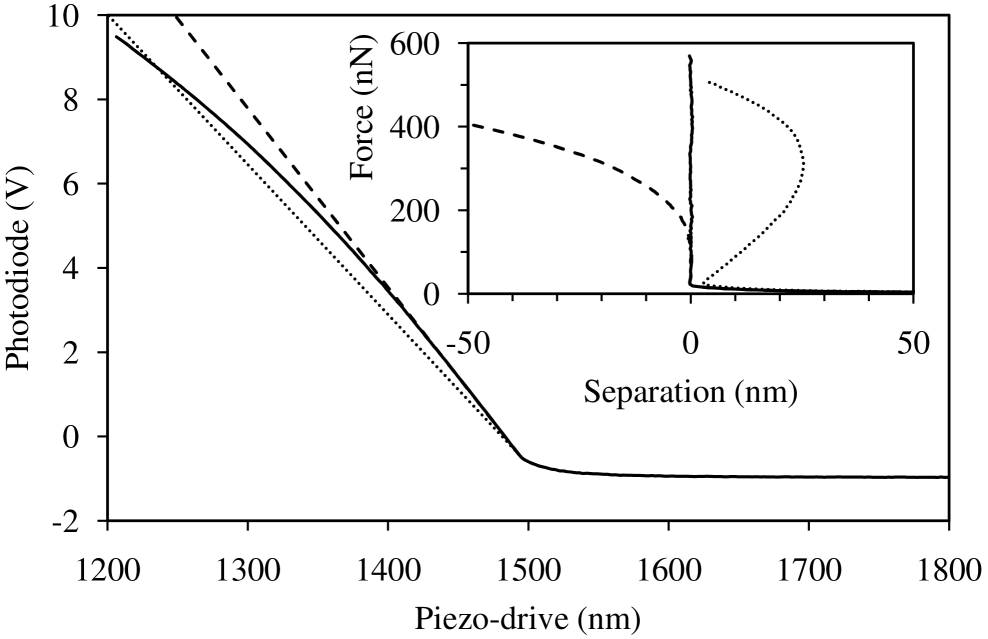
Figure 1: The raw photo-diode voltage versus the piezo-drive displacement. The solid curve is measured extension data, the dashed line is the tangent to the contact region at first contact, and the dotted line uses the average slope in contact. The inset shows the analysed force versus separation, with the solid curve resulting from the non-linear analysis (see text) and the dashed and dotted curves resulting from the conventional linear analysis using the first contact slope and the average slope, respectively. The source of the measured data is Ref. Zhu12, ; a summary of the experimental details is given in Ref. expt, .

To make this clear mathematically, let the measured constant compliance slope be

$$\beta\equiv\left.\frac{\Delta V}{\Delta z_{\mathrm{p}}}\right|_{\mathrm{contact}}.$$ (1)

Here $V$ is the photo-diode voltage and $z_{\mathrm{p}}$ is the piezo-drive position. Letting $V_{\mathrm{b}}$ be the base-line voltage far from contact, the surface force is

$$F(z_{\mathrm{p}})=-k_{0}\beta^{-1}[V(z_{\mathrm{p}})-V_{\mathrm{b}}],$$ (2)

where $k_{0}$ is the cantilever spring constant. The force goes to zero at large separations, which is the base-line region. This result invokes the fact that in hard contact the change in tip position is equal and opposite to the change in piezo-drive position, NB1 $\Delta z_{\mathrm{t}}=-\Delta z_{\mathrm{p}}$, and the force on the cantilever is $F=k_{0}z_{\mathrm{t}}$. (The simple presentation given here ignores a number of important linear effects such as base-line drift, friction in contact, cantilever tilt, and non-negligible base-line force. These and non-linear effects will be included in the more sophisticated linear and non-linear analysis below.) The separation is

$$h = z_{\mathrm{p}}+z_{\mathrm{t}}+\mbox{const}$$ (3)

$$= z_{\mathrm{p}}+k_{0}^{-1}F^{\mathrm{ext}}(z_{\mathrm{p}})+\mbox{const},$$

where the constant is chosen so that $h=0$ in contact.

It ought to be clear from the above how important the calibration factor $\beta$, which is the constant compliance slope, is to the quantitative measurement of surface forces with the atomic force microscope. However it is not unusual for the photo-diode voltage versus piezo-drive position curve to be non-linear in the contact region. A typical example is shown in Fig. 1. It is emphasised that the data in the figure were obtained for hard surfaces and so the curvature evident is not due to elastic deformation of the probe or substrate. A curved constant compliance region such as that in Fig. 1 creates several problems. At a minimum, the calibration factor $\beta$ is not unique; the slope depends upon where in the contact region it is measured, which introduces quantitative uncertainty into the linear analysis, (compare, for example, the result that uses the slope at first contact (dashed line and curve) with the result that uses the average slope (dotted line and curve)). Ambiguity also arises because the contact behavior differs between extension and retraction (not shown). Worse, a non-linear contact region contradicts the fundamental assumption of a linear response and raises questions about the conventional linear analysis that is used to quantify surface force measurements.

The inset to Fig. 1 graphically illustrates the problems with the linear analysis. It can be seen that it gives grossly unphysical non-zero separations in the contact region. In this case the surfaces are known to be rigid so the results is unambiguously unphysical. In other cases, where the surfaces are either of unknown rigidity or known to be soft, this artefact of the linear analysis would be misinterpreted as the elastic deformation of the material. Not only the elasticity but any useful physical information in the contact region is precluded by the linear analysis. As will be demonstrated below, the non-linear analysis can be used to obtain reliable values for properties like the friction coefficient, roughness, and topography of the contact region.

It is not only in contact that the linear analysis can fail. If a large surface force is present, then the linear analysis of the data introduces quantitative errors into the values of the surface force in the non-contact region. This can be a particular problem if one requires reliable and accurate surface force measurements, or if one seeks small changes in forces with control parameters, or if one needs to quantify second order effects. In all these cases the linear analysis can be unsuitable, depending upon the extent of the non-linearity and the magnitude of the forces.

The are two possible physical origins of the non-linearity displayed in Fig. 1. The first possibility is that the cantilever deflection becomes non-linear over the relatively large range of the contact region. By cantilever non-linearity is meant that the four relevant quantities (tip position, deflection, angle deflection, and force) are not linearly proportional to each other. The second possibility is a non-linear relationship between the change in photo-diode voltage and the change in cantilever angle. Since the change in voltage difference in the split photo-diode depends only on that part of the optical beam currently crossing the boundary (assuming uniform sensitivity of the photo-diode; any spatial variability in the sensitivity will contribute further to non-linearities), any variability in the spatial intensity or width of the beam (e.g. circular or elliptical cross-section, Gaussean intensity distribution) will give non-linear effects.

I.0.1 Contents

For the case of the rectangular cantilever, a complete linear analysis is given in §II. In §II.2, the effects of base-line drift, virtual deflection, cantilever tilt, friction in contact, and non-negligible base-line force are accounted for. These are often neglected in the conventional linear analysis. A new result is an algorithm for determining the zero of separation, §II.2.5. The effective spring constant that must be used in the linear analysis and its relation to the cantilever spring constant is given in §II.2.6. In §III.1 are given the non-linear equations for a rectangular cantilever that determine the deflection, deflection angle, vertical position, and applied force, taking into account tilt and friction. In §III.2 an algorithm suitable for spreadsheet use is given for the analysis of experimental data (i.e. the conversion from raw voltage versus piezo-drive position to force versus separation) in the case of non-linear behavior. The non-linearities can arise either from the non-linear cantilever deflection or the non-linear photo-diode response, or both. For the non-linear photo-diode case, the non-linearity is characterized by the measurement itself and it is not necessary to know the details of the source of the non-linearity. This is fortunate because unlike rectangular cantilevers, these vary between different models of the atomic force microscope. In §III.3 the case of a linear photo-diode and non-linear cantilever is explored numerically for the case shown in Fig. 1, and it is concluded that the non-linear cantilever deflection is insufficient to account for the measured non-linear effects. In §III.4, summarized are the equations for a linear cantilever and a non-linear photo-diode, which are somewhat simpler than the dual non-linear case. In §IV, these are applied to measured atomic force microscope data for the drainage force at several drive velocities. Results for the slip length and the drainage adhesion are obtained. The quantitative and qualitative differences between the linear and the non-linear analysis of the experimental data are shown.

II Linear Analysis

II.1 Horizontal Cantilever, No Friction

II.1.1 Deflection

The bending of a cantilever beam under the influence of fores and torques is one of the classic problems of the theory of elasticity. A beam of length $L_{0}$, and with a deflection $x$ and angular deflection $\theta$ has stored elastic energySouthwell36

$$U(x,\theta)=\frac{2B}{L_{0}^{3}}\left[3x^{2}-3xL_{0}\theta+L_{0}^{2}\theta^{2}\right].$$ (4)

The elastic parameter $B\equiv EI$ depends upon Young s modulus and the geometric second moment of the beam; it will be related to the spring constant of the cantilever beam below. Differentiating with respect to the deflection gives the force exerted on the end of the beam,

$$F\equiv\frac{\partial U(x,\theta)}{\partial x}=\frac{2B}{L_{0}^{3}}\left[6x-3L_{0}\theta\right].$$ (5)

and differentiating with respect to angle gives the torque

$$\tau\equiv\frac{\partial U(x,\theta)}{\partial\theta}=\frac{2B}{L_{0}^{3}}\left[-3L_{0}x+2L_{0}^{2}\theta\right].$$ (6)

These assume that the beam is in equilibrium with the applied forces and torques.

Inverting these equations gives the standard expressions for the deflection and the angle in terms of the applied force and torque,Southwell36

$$x=\frac{1}{2B}\left[\frac{2}{3}L_{0}^{3}F+L_{0}^{2}\tau\right],$$ (7)

and

$$\theta=\frac{1}{2B}\left[L_{0}^{2}F+2L_{0}\tau\right].$$ (8)

II.1.2 Spring Constant

One has to be a little cautious about assigning a spring constant. The above equations refer to a free, horizontal cantilever beam, and now the spring constant for such a beam with normal force and zero torque (free deflection) will be given. It is emphasized that this cannot be applied to the atomic force microscope without modification because in that case the cantilever beam is tilted, the force is not entirely normal to the beam, and there are non-zero torques due to this and due to friction. This case will be handled shortly.

For the horizontal beam with zero torque, $\tau=0$, the deflection is linearly proportional to the applied force, $x=[L_{0}^{3}/3B]F$, from which one can identify the cantilever spring constant as

$$k_{0}\equiv 3B/L_{0}^{3}.$$ (9)

In this paper the elastic parameter $B$ will be used, as it is an intrinsic property of the cantilever. Usually (but not always; see §II.2.6 below) any quoted or measured spring constant is the horizontal, free spring constant in the above sense, and so this equation can be used to convert from $k_{0}$ to $B$.

For free deflection, $\tau=0$, the angular deflection is linearly proportional to the deflection,

$$\theta=\frac{3}{2L_{0}}x.$$ (10)

This particular proportionality constant only holds for the free, horizontal cantilever. For the free tilted cantilever, the two remain linearly proportional to each other, but a different constant applies, as is derived below.

The linear proportionality of deflection angle $\theta$ and deflection $x$ underlies the linear analysis of atomic force microscope. The light lever is assumed to give a change in voltage that is linearly proportional to the deflection angle, $\gamma\equiv\Delta V/\Delta\theta$. Since the deflection angle, deflection, and force, are all linearly proportional to each other by the above two equations, then one can get the force from the measured change in voltage,

$$F=k_{0}x=\frac{2k_{0}L_{0}}{3}\theta=\frac{2k_{0}L_{0}}{3\gamma}\Delta V.$$ (11)

If the measured gradient of the photo-diode signal in contact is $\beta\equiv\Delta V/\Delta z_{\mathrm{p}}=-\Delta V/\Delta x$, then

$$\gamma=\frac{-2L_{0}}{3}\beta.$$ (12)

Hence $F=-k_{0}\beta^{-1}\Delta V$. This is the conventional linear analysis for extracting the force from of atomic force microscope measurements. It ought be clear it assumes a horizontal cantilever with no torque, neither of which assumption holds in practice.

II.1.3 Spring Constant Calibration

One of the most important issues in measuring forces with the atomic force microscope is the determination of the spring constant. This is usually the largest source of systematic error. The common thermal calibration procedureHiggins06 that is often built into the software of the atomic force microscope gives erroneous results, with a systematic overestimate of the spring constant of 15%–30%.Higgins06 ; Attard06a The source of the error in the derivation has been identified and a more reliable thermal calibration method has been given.Attard06a (The correct thermal calibration formula for the cantilever spring constant is given in Eq. (II.2.6) below.) An even more accurate and reliable way of determining the spring constant is to use the long range hydrodynamic drainage force. Zhu11a ; Zhu11b ; Craig01 In general the drainage force is known exactly, at least in the large separation regime

$$F_{\mathrm{drain}}(h)=\frac{-6\pi\eta R^{2}\dot{z}_{\mathrm{p}}}{h},$$ (13)

where $\eta$ is the viscosity. It is permissible to use the piezo-drive velocity $\dot{z}_{\mathrm{p}}$ rather than the rate of change of change of separation in this because the deflection is small and its rate of change is negligible at large separations. The correct spring constant gives agreement between this and the measured force at long range.

It should be noted that if this method of calibration is used in conjunction with the conventional analysis of the measured data (linear calibration, horizontal cantilever), then the spring constant that results is the effective spring constant $k_{\mathrm{eff}}$ rather than the intrinsic cantilever spring constant $k_{0}$. These are defined in the full analysis for the tilted cantilever with friction that is treated next.

II.2 Tilted Cantilever with Friction

II.2.1 Model

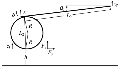
Figure 2: Cantilever geometry in the atomic force microscope (not to scale).

Following earlier work,Attard98 ; Attard99 the cantilever and probe in the atomic force microscope is modeled as in Fig. 2. The key features are the fixed tilt angle of the cantilever, $\theta_{0}<0$, such that the total angle of the cantilever is the sum of this and the deflection angle, $\theta_{\mathrm{tot}}=\theta_{0}+\theta$, and the rigid lever arm, $L_{2}(\theta_{\mathrm{tot}})$, which connects the cantilever to the point of application of the normal surface force $F_{z}$ and the lateral friction force $F_{y}$, if present. The force $F$ and torque $\tau$ on the cantilever treated in the preceding section are a function of these two forces, the lever arm, and the tilt angle, as will now be derived.

Note that in the figure the piezo-drive is connected to the base of the cantilever, so that extension corresponds to $\dot{z}_{\mathrm{p}}<0$ and retraction corresponds to $\dot{z}_{\mathrm{p}}>0$.NB1 The separation between the surfaces is

$$h\equiv z_{\mathrm{p}}+z_{\mathrm{t}}+z_{0}^{\mathrm{ext}},$$ (14)

with the constant $z_{0}^{\mathrm{ext}}$ calculated to give zero separation at first contact, as defined below. In contact, $\Delta h=0$, so that $\Delta z_{\mathrm{t}}=-\Delta z_{\mathrm{p}}$.NB1

Trigonometric functions of the tilt angle occur frequently below and so it is convenient to define fixed constants

$$C_{0}\equiv\cos\theta_{0}\mbox{, and }S_{0}\equiv\sin\theta_{0}.$$ (15)

Note that in the present geometry for the atomic force microscope, $S_{0}\approx\theta_{0}\approx-0.2$, which is small in magnitude and negative in sign. (All angles here and throughout are measured in radians; in degrees, $\theta_{0}\approx-11^{\circ}$.)

II.2.2 Friction Force

In this work the lateral force will be taken to be due to friction (in contact) and it will be taken to be linearly proportional to the load,

$$F_{y}=\left\{\begin{array}[]{ll}\mu F_{z},&\mbox{extension, contact},\\ -\mu F_{z},&\mbox{retraction, contact},\\ 0,&\mbox{non-contact}.\end{array}\right.$$ (16)

This is known as Amontons law. As drawn in Fig. 2, on extension $\dot{z}_{\mathrm{p}}<0$, and so in contact on extension $\dot{z}_{\mathrm{t}}>0$. This means that due to the tilt angle, $\dot{y}<0$ and $F_{y}>0$. Since in contact $F_{z}>0$ (at least sufficiently far into contact), this accounts for the sign of the first equality. (In general the friction coefficient is positive.) The opposite occurs on retraction ($\dot{y}>0$ and $F_{y}<0$), the second equality. Out of contact there is no friction.

The assumption that the friction force is linearly proportional to the load is a significant one. This is certainly the classical model of friction, at least at the macroscopic level. There is evidence in the atomic force microscope literature forStiernstedt05 and againstFeiler00 such an assumption. The former data is perhaps the most convincing as four independent measurements were made (two different colloid probes, two different friction measurement methods).

Immediately after the initial contact on extension, and at the beginning of the retraction branch in contact (the turn point), the probe is not moving at uniform velocity and so the assumed form for the friction force will produce artifacts at these points in the analyzed data. Also, when the force at either first or last contact is non-zero, the model gives a discontinuity in the friction force and consequently a discontinuity in the surface force that is also an artefact of the simple model.

All the following results will be given explicitly for extension in contact. The retraction results may be obtained by the replacement $\mu\Rightarrow-\mu$, and the non-contact results may be obtained by the replacement $\mu\Rightarrow 0$. The superscripts ‘ext’ (contact, $\mu>0$), ‘ret’ (contact, $\mu<0$), and ‘nc’ (non-contact, $\mu=0$) will often be used to denote each of the three cases. For the voltage, the piezo-drive position, and the surface force, which is possibly velocity dependent, the superscripts ‘ext’ and ‘ret’ will be used also in the non-contact situation. The subscript ‘c’ denotes a quantity in contact, and the subscript ‘b’ denotes a quantity in the base-line region far from contact.

II.2.3 Linear Cantilever Equations

In Eqs (45) and (46) below, non-linear expressions are derived for the deflection, the angular deflection, and the force. In the linear regime one can simply make the replacement $\theta_{\mathrm{tot}}\Rightarrow\theta_{0}$ to obtain

$$x=\left\{\frac{L_{0}^{3}}{3B}\left[C_{0}+\mu S_{0}\right]+\frac{L_{0}^{2}L_{2}}{2B}\left[S_{0}-\mu C_{0}\right]\right\}F_{z},$$ (17)

and

$$\theta = \left\{\frac{L_{0}^{2}}{2B}\left[C_{0}+\mu S_{0}\right]+\frac{L_{0}L_{2}}{B}\left[S_{0}-\mu C_{0}\right]\right\}F_{z}$$ (18)

$$\equiv E^{\mathrm{ext}}F_{z}.$$

Here the length of the lever arm in the undeflected state is $L_{2}\equiv L_{2}(\theta_{0})=R\sqrt{2+2\cos\theta_{0}}$. In the linear regime, the force, deflection, and deflection angle are linearly proportional to each other. In particular it is convenient to define the proportionality constant between deflection and deflection angle from

$$x = \frac{2L_{0}^{3}[C_{0}+\mu S_{0}]+3L_{0}^{2}L_{2}[S_{0}-\mu C_{0}]}{3L_{0}^{2}[C_{0}+\mu S_{0}]+6L_{0}L_{2}[S_{0}-\mu C_{0}]}\theta$$ (19)

$$\equiv D^{\mathrm{ext}}\theta.$$

In general $L_{2}\ll L_{0}$, and this and the above results could be expanded to linear order in $L_{2}/L_{0}$. There is no great advantage in doing this.

The vertical position of the tip depends upon the deflection, the deflection angle, and the length of the lever arm, Eq. (40) below. The linearized form of Eq. (39) for the length of the lever arm is $L_{2}(\theta_{\mathrm{tot}})=L_{2}-{R^{2}S_{0}}\theta/{L_{2}}$. For the case of a tipped cantilever, $L_{2}(\theta_{\mathrm{tot}})$ is equal to the length of the tip, and there is no dependence on the deflection angle (i.e. the term in $R^{2}$ may be set to zero). Linearising Eq. (40) below for the vertical tip position yields

$$z_{\mathrm{t}} = C_{0}x+\left[L_{2}S_{0}-\frac{R^{2}S_{0}^{2}\theta_{0}}{L_{2}}+L_{2}C_{0}\theta_{0}\right]\theta$$ (20)

$$= \left\{D^{\mathrm{ext}}C_{0}+L_{2}S_{0}-\frac{R^{2}S_{0}^{2}\theta_{0}}{L_{2}}+L_{2}C_{0}\theta_{0}\right\}\theta$$

$$\equiv \theta/\alpha^{\mathrm{ext}}.$$

The proportionality constant is $\alpha\equiv\mathrm{d}\theta/\mathrm{d}z_{\mathrm{t}}$. It has a different value for each of the three cases $\mu>0$ (contact, extension), $\mu<0$ (contact, retraction), and $\mu=0$ (non-contact).

II.2.4 Linear Analysis of Measured Data

The measured data in the atomic force microscope consists of the raw photo-diode voltage $\tilde{V}(t)$ and the piezo-drive position $z_{\mathrm{p}}(t)$. These are both a function of time, and so the voltage may equivalently be regarded as a function of position, $\tilde{V}(z_{\mathrm{p}})$. One has in fact two sets of data, one for extend, $\tilde{V}^{\mathrm{ext}}(z_{\mathrm{p}})$, and one for retract, $\tilde{V}^{\mathrm{ret}}(z_{\mathrm{p}})$. Only the equations for extension will be shown explicitly here.

The tilde on the voltage is used to denote the raw measured voltage. The raw voltage contains contributions from the change in angle of the cantilever and from various artifacts that include a constant voltage off-set, thermal drift, and virtual deflection.Zhu11a ; Zhu11b Two further physical effects have to be carefully accounted for, namely the drag force on the cantilever and the long range asymptote of the surface force. The deflection angle of the cantilever due to the surface forces is what is desired to extract from the measured voltage. The notation $V(z_{\mathrm{p}})$ will be used to denote the measured voltage that has been corrected for these various artifacts and forces.

In the base-line region, where the surfaces are far from contact, the surface force is small and in many cases negligible. Hence almost all of the measured voltage in this region is due to the artifacts just mentioned. These in general are linear functions of position, and one can define the measured base-line voltage on extension as

$$\tilde{V}^{\mathrm{ext}}_{\mathrm{b}}(z_{\mathrm{p}})=\tilde{V}^{\mathrm{ext}}_{\mathrm{b}}+\tilde{\beta}^{\mathrm{ext}}_{\mathrm{b}}[z_{\mathrm{p}}-z_{\mathrm{pb}}],$$ (21)

and similarly for retraction. The base-line slope is $\tilde{\beta}^{\mathrm{ext}}_{\mathrm{b}}\equiv\left.\mathrm{d}\tilde{V}^{\mathrm{ext}}(z_{\mathrm{p}})/\mathrm{d}z_{\mathrm{p}}\right|_{z_{\mathrm{pb}}}$. The coefficients for this are obtained by a linear fit to the measured data in an interval about the fixed position $z_{\mathrm{pb}}$ in the base-line region. Once the coefficients are determined, this linear fit is applied to the whole measured regime, not just the base-line region (because the artifacts that it removes apply to the whole regime). With this the corrected voltage on extension is

$$V^{\mathrm{ext}}(z_{\mathrm{p}})=\tilde{V}^{\mathrm{ext}}(z_{\mathrm{p}})-\tilde{V}^{\mathrm{ext}}_{\mathrm{b}}(z_{\mathrm{p}}).$$ (22)

This is zero in the base-line region.

This expression removes from the raw signal not only the artifacts mentioned above but also the constant drag force. (In some cases the drag force is not constant.Zhu11a ; Zhu11b This effect, which can be important for cantilevers with a low spring constant, is not included in the present analysis.) It also removes the linear extrapolation of the asymptote of surface force,

$$F^{\mathrm{ext}}_{\mathrm{b}}(z_{\mathrm{p}})=F^{\mathrm{ext}}_{\mathrm{b}}+F^{\mathrm{ext^{\prime}}}_{\mathrm{b}}[z_{\mathrm{p}}-z_{\mathrm{pb}}].$$ (23)

Here the constant force is $F^{\mathrm{ext}}_{\mathrm{b}}=F^{\mathrm{ext}}(h_{\mathrm{b}})$ and the derivative is $F^{\mathrm{ext^{\prime}}}_{\mathrm{b}}=\mathrm{d}F^{\mathrm{ext}}(h_{\mathrm{b}})/\mathrm{d}h_{\mathrm{b}}$, where the separation is $h_{\mathrm{b}}=z_{\mathrm{pb}}+z_{0}^{\mathrm{ext}}$. (This neglects the deflection of the cantilever, which should be negligible; if not, add to the separation $z_{\mathrm{tb}}\approx F^{\mathrm{ext}}_{\mathrm{b}}/k_{0}$.) In almost all cases this extrapolated surface force from the base-line region is negligible. In those cases where it isn’t, it has to be added back, as will be done shortly.

The contact region is where the separation between the surfaces is zero, and the tip moves equal and opposite to the piezo-drive, $\Delta z_{\mathrm{t}}=-\Delta z_{\mathrm{p}}$.NB1 In the linear regime, the slope is constant and this is also called the constant compliance regime. It does not matter whether one fits the raw data or the corrected data because the two contact slopes are related by

$$\beta^{\mathrm{ext}}_{\mathrm{c}}\equiv\frac{\Delta V^{\mathrm{ext}}_{\mathrm{c}}}{\Delta z_{\mathrm{p}}},\;\;\tilde{\beta}^{\mathrm{ext}}_{\mathrm{c}}\equiv\frac{\Delta\tilde{V}^{\mathrm{ext}}_{\mathrm{c}}}{\Delta z_{\mathrm{p}}},\;\;\beta^{\mathrm{ext}}_{\mathrm{c}}=\tilde{\beta}^{\mathrm{ext}}_{\mathrm{c}}-\tilde{\beta}^{\mathrm{ext}}_{\mathrm{b}}.$$ (24)

If a positive voltage corresponds to a repulsive force, then the slope ought to be negative.

The light lever measures the angle of the cantilever. The key to analyzing atomic force microscope force data is to calibrate the light lever by measuring the proportionality constant between angle and photo-diode voltage,

$$\gamma\equiv\frac{\Delta V}{\Delta\theta}.$$ (25)

This is the same on extension and retraction, and it is the same in contact and out of contact. This expression assumes a linear photo-diode, but not necessarily a linear cantilever.

The value of this conversion factor follows from the measured slope in contact, Eq. (24), and the linear proportionality between angular deflection and tip position, Eq. (20). Evaluating these on extension in contact one has

$$\gamma^{\mathrm{ext}}=\frac{\Delta V}{\Delta z_{\mathrm{p}}}\frac{\Delta z_{\mathrm{p}}}{\Delta z_{\mathrm{t}}}\frac{\Delta z_{\mathrm{t}}}{\Delta\theta}=-\beta^{\mathrm{ext}}_{\mathrm{c}}/\alpha^{\mathrm{ext}}.$$ (26)

One has a similar result for retraction in contact $\gamma^{\mathrm{ret}}=-\beta^{\mathrm{ret}}_{\mathrm{c}}/\alpha^{\mathrm{ret}}$. Since this has to be a property of the light lever, the value of $\gamma$ cannot depend upon whether or not the surfaces are in contact, or whether the measurement is made on extension or on retraction. Hence one must have $\gamma^{\mathrm{ext}}=\gamma^{\mathrm{ret}}$, or

$$\frac{\beta^{\mathrm{ext}}_{\mathrm{c}}}{\beta^{\mathrm{ret}}_{\mathrm{c}}}=\frac{\alpha(\mu)}{\alpha(-\mu)},$$ (27)

since $\alpha^{\mathrm{ext}}=\alpha(\mu)$ and $\alpha^{\mathrm{ret}}=\alpha(-\mu)$. The left hand side is a measured quantity, and the right hand side is a known non-linear function of $\mu$, Eq. (20). There exist sophisticated algorithms for solving such non-linear equations, with perhaps the most common if not the most powerful being to guess the solution. (This can be turned into a quadratic equation for $\mu$ if one expands $D(\mu)$ to leading order in $L_{2}/L_{0}$. There is a small loss of accuracy in such an expansion, which is not compensated by the even smaller gain of an explicit analytic solution.) This result provides a way of measuring the friction coefficient.

With $\gamma$ having been obtained from the measured contact slope and the calculated rate of change of tip position with angle, Eq. (26), one can now give the surface force as a function of separation. From Eq. (18), the angle deflection is

$$\theta^{\mathrm{ext}}(z_{\mathrm{p}})=\gamma^{-1}V^{\mathrm{ext}}(z_{\mathrm{p}})+E^{\mathrm{nc}}F^{\mathrm{ext}}_{\mathrm{b}}(z_{\mathrm{p}}).$$ (28)

Here the contribution of the linear extrapolation of the asymptote of the surface force, $F^{\mathrm{ext}}_{\mathrm{b}}(z_{\mathrm{p}})$, which is assumed a known function and which was removed from the raw voltage signal, has been added back to give the full deformation angle. Note that it is the non-contact value of the conversion factor, $E^{\mathrm{nc}}=E(\mu=0)$ that is used here. Inserting this into Eq. (18) gives the surface force $F^{\mathrm{ext}}(z_{\mathrm{p}})$. Explicitly in terms of the voltage it is

$$F^{\mathrm{ext}}(z_{\mathrm{p}})=\left\{\begin{array}[]{cc}\displaystyle\frac{1}{E^{\mathrm{nc}}\gamma}V^{\mathrm{ext}}(z_{\mathrm{p}})+F^{\mathrm{ext}}_{\mathrm{b}}(z_{\mathrm{p}}),&h>0,\\ \displaystyle\frac{1}{E^{\mathrm{ext}}\gamma}V^{\mathrm{ext}}(z_{\mathrm{p}})+F^{\mathrm{ext}}_{\mathrm{b}}(z_{\mathrm{p}}),&h=0.\end{array}\right.$$ (29)

From Eq. (20) the separation is

$$h^{\mathrm{ext}}(z_{\mathrm{p}}) = z_{\mathrm{p}}+\frac{1}{\alpha^{\mathrm{nc}}}\theta^{\mathrm{ext}}(z_{\mathrm{p}})+z_{0}^{\mathrm{ext}}$$

$$= z_{\mathrm{p}}+\frac{1}{\alpha^{\mathrm{nc}}\gamma}V^{\mathrm{ext}}(z_{\mathrm{p}})+\frac{E^{\mathrm{nc}}}{\alpha^{\mathrm{nc}}}F^{\mathrm{ext}}_{\mathrm{b}}(z_{\mathrm{p}})+z_{0}^{\mathrm{ext}}.$$

The constant $z_{0}^{\mathrm{ext}}$ is calculated so that $h^{\mathrm{ext}}=0$ when the surfaces first come into contact (see next). The separation equation is normally used explicitly for $h>0$. These three equations are written explicitly for extension; for retraction in contact change the superscript ‘ext’ to ‘ret’, including $E^{\mathrm{ext}}\equiv E(\mu)\Rightarrow E^{\mathrm{ret}}\equiv E(-\mu)$.

II.2.5 Zero of Separation

The constant $z_{0}^{\mathrm{ext}}$ remains to be determined. The conventional way of establishing the zero of separation is by eye, which is to say the force curve is shifted horizontally until it looks ‘right’. The problem with this is that there is often ambiguities in identifying first contact, particularly when one has a steeply repulsive surface force prior to contact. Also the constant that gives $h=0$ at first contact may be different to the constant that gives $h=0$ for most of the contact region, even when the correct friction coefficient is used, as will be demonstrated by explicit data below. Finally, choosing the zero of separation by eye introduces a psychological element into the analysis and the potential for personal bias that would be best removed by having a mathematical algorithm for finding contact.

It may be objected that identifying the contact and the base-line regions already introduce some form of psychological bias into the analysis of the experimental data. However, it turns out that the various fits are not very sensitive to the choice of the region used for the fit, within reason, and the result do not vary significantly with different choices. The zero of separation, however, feeds directly into the final result, and a difference of as small as 1 nm can quantitatively effect the values of parameters that one is trying to measure (e.g. the slip length in drainage flow can be of the same order), and it can even qualitatively effect the physical interpretation of the data.

The strategy is to define $z_{0}^{\mathrm{ext}}$ so that the separation is exactly zero at first contact, (and to define $z_{0}^{\mathrm{ret}}$ so that $h=0$ at last contact). ‘First’ (or ‘last’) contact is defined to mean the point at which the extrapolated base-line voltage intersects the extrapolated contact voltage. This definition is precise and unambiguous, it is able to be calculated mathematically, and it is physically reasonable and in accord with one intuitive understanding of the meaning of contact.

It should be understood that there are conceptual problems with the meaning of ‘separation’ at the molecular level. The separation as defined here, $h\equiv z_{\mathrm{p}}+z_{\mathrm{t}}+z_{0}$, is not precisely zero over the whole contact region. It rather measures the difference between changes in the piezo-drive position and changes in the tip position. It is positive when there is a protuberance on the substrate, and it is negative when there is a depression. It is also negative when compression of a deformable surface occurs. Hence the separation $h$ in contact really gives a topographic map of the substrate. The zero plane of the map is here defined as the plane passing through the point of first or last contact.

Let $z_{\mathrm{pc}}^{\mathrm{ext}}$ be the piezo-drive position at first contact, and let $V_{\mathrm{c}}^{\mathrm{ext}}=V^{\mathrm{ext}}(z_{\mathrm{pc}}^{\mathrm{ext}})$ be the corrected voltage at first contact. (In the linear case, it makes no difference to the results what point is selected for $z_{\mathrm{pc}}^{\mathrm{ext}}$.) In contact, $V^{\mathrm{ext}}(z_{\mathrm{p}})=V_{\mathrm{c}}^{\mathrm{ext}}+\beta_{\mathrm{c}}^{\mathrm{ext}}[z_{\mathrm{p}}-z_{\mathrm{pc}}^{\mathrm{ext}}]$. The position at which the voltage in contact extrapolates to zero, which is defined as first contact, is

$$z_{\mathrm{pcb}}^{\mathrm{ext}}=z_{\mathrm{pc}}^{\mathrm{ext}}-V_{\mathrm{c}}^{\mathrm{ext}}/\beta_{\mathrm{c}}^{\mathrm{ext}}.$$ (31)

(The base-line corrected voltage is zero, and so this is the same as the intersection of the base-line and contact raw voltages.) When the voltage is zero the angular deflection is

$$\theta^{\mathrm{ext}}(z_{\mathrm{pcb}}^{\mathrm{ext}})=E^{\mathrm{nc}}F^{\mathrm{ext}}_{\mathrm{b}}(z_{\mathrm{pcb}}^{\mathrm{ext}}).$$ (32)

Inserting this into the equation for the separation, and setting the latter to zero, $h^{\mathrm{ext}}(z_{\mathrm{pcb}}^{\mathrm{ext}})=0$, gives the shift constant,

$$z_{0}^{\mathrm{ext}}=-z_{\mathrm{pcb}}^{\mathrm{ext}}-\frac{E^{\mathrm{nc}}}{\alpha^{\mathrm{nc}}}F^{\mathrm{ext}}_{\mathrm{b}}(z_{\mathrm{pcb}}^{\mathrm{ext}}).$$ (33)

II.2.6 Effective Spring Constant

The conventional modeling of the atomic force microscope is not only linear but also effectively takes the cantilever to be horizontal. Ignoring the tilt is equivalent to equating the cantilever deflection to the vertical position of the tip, $x\equiv z_{\mathrm{t}}$. The relationship between the measured photo-diode voltage and the vertical tip position is given by the calibration factor obtained from the slope of the contact region. In this case, the effective spring constant that gives the non-contact force is

$$k_{\mathrm{eff}}\equiv\frac{F_{z}}{z_{\mathrm{t}}}=\alpha^{\mathrm{nc}}/E^{\mathrm{nc}}.$$ (34)

The constants $E^{\mathrm{nc}}\equiv E(\mu=0)$ and $\alpha^{\mathrm{nc}}\equiv\alpha(\mu=0)$ are defined in Eqs (18) and (20), respectively.

The difference between the cantilever spring constant $k_{0}=3B/L_{0}^{3}$ and the effective spring constant $k_{\mathrm{eff}}$ can be substantial. For the case analyzed in detail below ($L_{0}=110\,\mu$m, $R=10.1\,\mu$m, $\theta_{0}=-11^{\circ}$), the cantilever spring constant is $k_{0}=1.37\,$N/m and the effective spring constant is $k_{\mathrm{eff}}=1.68\,$N/m.

In using the equations for the tilted cantilever to convert measured atomic force microscope data to force, one should use the cantilever spring constant. In using the equations for the horizontal cantilever (simple spring model, the conventional approach) to convert measured atomic force microscope data to force, one should use the effective spring constant. In calculating a theoretical force curve modeled with the cantilever as a simple spring, one should also use the effective spring constant.

Finally, in Ref. Attard06a, the correct equations for the thermal calibration of the atomic force microscope cantilever were given. In that paper the cantilever spring constant was denoted $k_{0}$ (here also denoted $k_{0}$), and the effective force measuring spring constant was denoted $k$ (here denoted $k_{\mathrm{eff}}$) and was given in terms of the cantilever spring constant in Eq. (17) of Ref. Attard06a, . In the present notation, the correct thermal calibration method gives the cantilever spring constant as

$$k_{0} = \left\{\frac{-2\beta_{\mathrm{cb}}L_{0}}{3[C_{0}+2L_{2}S_{0}/L_{0}]}\right.$$

$$\mbox{ }\times\left.0.7830\sqrt{\frac{6k_{\mathrm{B}}T}{\pi L_{0}^{2}f_{\mathrm{R}}P_{\mathrm{DC}}Q}}\right.$$

$$\mbox{ }\times\left.\left[C_{0}^{2}+(3L_{2}S_{0}C_{0}/L_{0})+3S_{0}^{2}L_{2}^{2}/L_{0}^{2}\right]\rule{0.0pt}{14.22636pt}\right\}^{2}.$$

Here the measured quantities are $\beta_{\mathrm{cb}}=\Delta V/\Delta z_{\mathrm{p}}$, which is the contact slope evaluated near the base-line voltage, (the average of the extend and retract values), $f_{\mathrm{R}}$, which is the resonance frequency of the first mode in Hz, $P_{\mathrm{DC}}$, which is the direct current power response in V${}^{2}\,$Hz^-1, and $Q$, which is the quality factor. The length of the rigid part at the end of the cantilever, $L_{1}$, defined in earlier analysesAttard98 ; Attard99 ; Attard06a has here and throughout been set to zero.

This inserted into Eq. (34) gives the effective spring constant for use when the cantilever is modeled as a simple spring (i.e. tilt neglected), which is usually the case in the linear analysis of measured data and the theoretical modeling of force-separation curves.

II.2.7 Effective Drag Length

The above procedure for analyzing the measured data removes the constant force due to the drag on the cantilever from the extension data, and its equal and opposite value from the retraction data. In some case it is useful to have available an explicit value for this drag force.

Like the drainage force, and unlike the virtual deflection, the contribution to the gradient of the base-line due to thermal drift is equal and opposite on extension and retraction.

With $\tilde{\beta}_{\mathrm{b}}^{\mathrm{ext}}$ and $\tilde{\beta}_{\mathrm{b}}^{\mathrm{ret}}$ being the measured base-line slopes of the raw voltage as defined above, and $F_{\mathrm{b}}^{\mathrm{ext^{\prime}}}=-F_{\mathrm{b}}^{\mathrm{ret^{\prime}}}$ being the gradient of the drainage force in the base-line region, then the gradient of the voltage due to thermal drift is

$$\frac{\mathrm{d}\tilde{V}^{\mathrm{ext}}_{\mathrm{th}}}{\mathrm{d}z_{\mathrm{p}}}=\frac{1}{2}\left[\tilde{\beta}_{\mathrm{b}}^{\mathrm{ext}}-\tilde{\beta}_{\mathrm{b}}^{\mathrm{ret}}\right]-\frac{\gamma_{\mathrm{b}}E^{\mathrm{nc}}}{2}\left[F_{\mathrm{b}}^{\mathrm{ext^{\prime}}}-F_{\mathrm{b}}^{\mathrm{ret^{\prime}}}\right].$$ (36)

This is equal and opposite to the gradient on retraction. With $z_{\mathrm{p,turn}}$ being the turn point at the end of the extend branch and the beginning of the retract branch, it is readily shown that the constant drag force on extension is

$$F_{\mathrm{drag}}^{\mathrm{ext}} = -F_{\mathrm{b}}^{\mathrm{ext}}+\frac{1}{2\gamma E^{\mathrm{nc}}}\left[\tilde{V}_{\mathrm{b}}^{\mathrm{ext}}-\tilde{V}_{\mathrm{b}}^{\mathrm{ret}}\right]$$

$$\mbox{ }-\frac{1}{2\gamma E^{\mathrm{nc}}}\frac{\mathrm{d}\tilde{V}^{\mathrm{ext}}_{\mathrm{th}}}{\mathrm{d}z_{\mathrm{p}}}\left[2z_{\mathrm{p,turn}}-z_{\mathrm{pb}}^{\mathrm{ext}}-z_{\mathrm{pb}}^{\mathrm{ret}}\right].$$

One can define an effective drag length from

$$F_{\mathrm{drag}}^{\mathrm{ext}}\equiv-6\pi\eta\dot{z}_{\mathrm{p}}^{\mathrm{\,ext}}L_{\mathrm{eff}}.$$ (38)

One should not take $L_{\mathrm{eff}}$ too literally, but it is expected to be somewhat less than the length of the cantilever, typically one third to one half of $L_{0}$. It should be independent of the drive velocity, although because it is derived from the difference in the base-line values, it can have relative large errors, on the order of 10–20% (see results below).

III Non-Linear Cantilever or Photo-diode

III.1 Non-Linear Cantilever

For a spherical colloid probe of radius $R$, simple geometry, Fig. 2, gives the lever arm as

$$L_{2}(\theta_{\mathrm{tot}})=R\sqrt{2+2\cos(\theta_{0}+\theta)}.$$ (39)

In the undeflected state this will be written $L_{2}\equiv L_{2}(\theta_{0})=R\sqrt{2+2\cos\theta_{0}}$. For the case of a tipped cantilever, $L_{2}(\theta_{\mathrm{tot}})$ is equal to the length of the tip, and there is no dependence on the deflection angle. In fact, even for a spherical probe the dependence on angle is practically negligible, and $L_{2}(\theta_{\mathrm{tot}})$ can be replaced by $L_{2}$, or even by $2R$.

The vertical position of the tip depends upon the deflection and the deflection angle. Again simple geometry shows that

$$z_{\mathrm{t}}=x\cos\theta_{\mathrm{tot}}+L_{2}(\theta_{\mathrm{tot}})\sin(\theta_{\mathrm{tot}})\theta_{\mathrm{tot}}-L_{2}S_{0}\theta_{0}.$$ (40)

Since it is the change in tip position that is important, this has been chosen to be zero in the non-deflected state. This equation is the major source of non-linearity in the cantilever.

The force $F$ and torque $\tau$ on the cantilever, which were treated in §II.1, are a linearly proportional to the normal force $F_{z}$ and to the lateral force $F_{y}$, with the proportionality constant depending upon the lever arm and the tilt angle,

$$F=F_{z}\cos\theta_{\mathrm{tot}}+F_{y}\sin\theta_{\mathrm{tot}},$$ (41)

and

$$\tau=F_{z}L_{2}(\theta_{\mathrm{tot}})\sin\theta_{\mathrm{tot}}-F_{y}L_{2}(\theta_{\mathrm{tot}})\cos\theta_{\mathrm{tot}}.$$ (42)

Using the linear model of friction, $F_{y}=\pm\mu F_{z}$, §II.2.2, the force and torque are linearly proportional to the surface force $F_{z}$. For extension in contact one has

$$F=\left[\cos\theta_{\mathrm{tot}}+\mu\sin\theta_{\mathrm{tot}}\right]F_{z},$$ (43)

and

$$\tau=L_{2}(\theta_{\mathrm{tot}})\left[\sin\theta_{\mathrm{tot}}-\mu\cos\theta_{\mathrm{tot}}\right]F_{z}.$$ (44)

(Of course for retraction in contact, $\mu\Rightarrow-\mu$, and out of contact, $\mu=0$.) Inserting these into the standard cantilever equations (7) and (8) gives the deflection and deflection angle as linearly proportional to the normal force (on extension in contact),

$$x = \left\{\frac{L_{0}^{3}}{3B}\left[\cos\theta_{\mathrm{tot}}+\mu\sin\theta_{\mathrm{tot}}\right]\right.$$ (45)

$$\left.\mbox{ }+\frac{L_{0}^{2}L_{2}(\theta_{\mathrm{tot}})}{2B}\left[\sin\theta_{\mathrm{tot}}-\mu\cos\theta_{\mathrm{tot}}\right]\right\}F_{z},$$

and

$$\theta = \left\{\frac{L_{0}^{2}}{2B}\left[\cos\theta_{\mathrm{tot}}+\mu\sin\theta_{\mathrm{tot}}\right]\right.$$ (46)

$$\left.\mbox{ }+\frac{L_{0}L_{2}(\theta_{\mathrm{tot}})}{B}\left[\sin\theta_{\mathrm{tot}}-\mu\cos\theta_{\mathrm{tot}}\right]\right\}F_{z}.$$

Because the total angle depends upon the deflection angle, $\theta_{\mathrm{tot}}=\theta_{0}+\theta$, these represent a non-linear relationship between the force, deflection, and deflection angle. This last equation is best written by taking the proportionality function over to the other side, which gives the force as an explicit non-linear function of the deflection angle, $F_{z}(\theta)$.

III.2 Non-Linear Analysis of Measured Data

The non-linear analysis in this section holds for both sources of non-linearity: the cantilever treated explicitly in the preceding subsection and the photo-diode non-linearity, for which no specific model is given. In later sub-sections, one or other of these will be turned off.

The raw measured voltage $\tilde{V}$ is a non-linear function of the effective total angle, $\tilde{\theta}_{\mathrm{tot}}=\theta_{\mathrm{tot}}+\theta_{\mathrm{b}}-\theta_{\mathrm{bf}}=\theta_{0}+\theta+\theta_{\mathrm{b}}-\theta_{\mathrm{bf}}$. Note the distinction between the physical or relevant total angle $\theta_{\mathrm{tot}}$ and the effective total angle $\tilde{\theta}_{\mathrm{tot}}$. The physical contributions are the tilt angle $\theta_{0}$, which is known, and the deflection angle due to the surface force, $\theta$, which is to be obtained. The base-line angle $\theta_{\mathrm{b}}$ is essentially an artifact arising from thermal drift and virtual deflection, and it includes the angle due to drag force, here assumed constant (but see Refs. Zhu11a, ; Zhu11b, , where variable drag is shown to occur for weak cantilevers), and the angle deflection due to the linearly extrapolated asymptote of the surface force, $\theta_{\mathrm{bf}}$. In the non-linear case, whether it be the non-linear cantilever or the non-linear photo-diode, one cannot just subtract the base-line voltage from the raw voltage to obtain a corrected voltage that gives $\theta$ directly. However, the total angle is a linear function its component parts, and so the immediate tasks are to obtain the effective total angle from the measured raw voltage, $\tilde{\theta}_{\mathrm{tot}}(\tilde{V})$, and to obtain the base-line angle as a function of the piezo-drive position, $\theta_{\mathrm{b}}(z_{\mathrm{p}})$.

Do a non-linear fit of the measured photo-diode voltage in the contact region on extension,

$$z_{\mathrm{pc}}^{\mathrm{ext}}(\tilde{V})=a_{0}^{\mathrm{ext}}+a_{1}^{\mathrm{ext}}\tilde{V}+a_{2}^{\mathrm{ext}}\tilde{V}^{2}+a_{3}^{\mathrm{ext}}\tilde{V}^{3}+\ldots$$ (47)

It is best not to use too many terms in the fit. Also one should be certain that the fit begins just after first contact, and that it ends before any anomalies associated with the turn around point at the end of the extension branch.

In the non-linear cantilever case, one regards the angular deflection $\theta$ as the independent variable. From the non-linear Eq. (46), one can calculate the surface force $F_{z}(\theta)$, and inserting this into the non-linear Eq. (45) one can calculate the deflection $x(\theta)$. Inserting these into the non-linear equation Eq. (40) one can calculate the tip position $z_{\mathrm{t}}(\theta)$. Hence from these non-linear cantilever equations, $z_{\mathrm{t}}(\theta;\mu)$ is easily calculated. A non-linear fit can be made to this, (in contact and on extension, $\mu>0$),

$$\theta^{\mathrm{ext}}_{\mathrm{c}}(z_{\mathrm{t}})=b_{1}^{\mathrm{ext}}z_{\mathrm{t}}+b_{2}^{\mathrm{ext}}z_{\mathrm{t}}^{2}+b_{3}^{\mathrm{ext}}z_{\mathrm{t}}^{3}+\ldots$$ (48)

The leading coefficient is $b_{1}^{\mathrm{ext}}=\alpha^{\mathrm{ext}}$, which was given analytically in Eq. (20). One has $\theta^{\mathrm{ext}}_{\mathrm{tot,c}}(z_{\mathrm{t}})=\theta_{0}+\theta^{\mathrm{ext}}_{\mathrm{c}}(z_{\mathrm{t}})$.

As in the linear case, the measured voltage is fitted to a straight line in the base-line region, Eq. (21),

$$\tilde{V}^{\mathrm{ext}}_{\mathrm{b}}(z_{\mathrm{p}})=\tilde{V}^{\mathrm{ext}}_{\mathrm{b}}+\tilde{\beta}^{\mathrm{ext}}_{\mathrm{b}}[z_{\mathrm{p}}-z_{\mathrm{pb}}].$$ (49)

Now the raw contact slope from the non-linear fit Eq. (47), evaluated at the base-line voltage constant, $\tilde{V}^{\mathrm{ext}}_{\mathrm{b}}$ (possibly an extrapolation beyond the region of the fit), is

$$\tilde{\beta}_{\mathrm{cb}}^{\mathrm{ext}} \equiv \left.\frac{\Delta\tilde{V}_{\mathrm{c}}^{\mathrm{ext}}}{\Delta z_{\mathrm{p}}}\right|_{\tilde{V}_{\mathrm{b}}^{\mathrm{ext}}}$$ (50)

$$= \frac{1}{a_{1}^{\mathrm{ext}}+2a_{2}^{\mathrm{ext}}\tilde{V}^{\mathrm{ext}}_{\mathrm{b}}+3a_{3}^{\mathrm{ext}}(\tilde{V}^{\mathrm{ext}}_{\mathrm{b}})^{2}+\ldots}.$$

The tip position is a linear function of the deflection angle in the base-line region, and the gradient is

$$\alpha_{\mathrm{b}}^{\mathrm{nc}} \equiv \left.\frac{\mathrm{d}\theta}{\mathrm{d}z_{\mathrm{t}}}\right|_{z_{\mathrm{t}}=0}$$

$$= \frac{1}{D^{\mathrm{nc}}C_{0}+L_{2}S_{0}+L_{2}C_{0}\theta_{0}-{R^{2}S_{0}^{2}\theta_{0}}/{L_{2}}},$$

where $D^{\mathrm{nc}}=D(0)=[2L_{0}^{3}C_{0}+3L_{0}^{2}L_{2}S_{0}]/[3L_{0}^{2}C_{0}+6L_{0}L_{2}S_{0}]$, as follow from Eqs (19) and (20).

The raw voltage is the same function of the total angle in and out of contact, and on extension and on retraction. Hence the rate of change of raw voltage with total angle (equivalently, deflection angle) in the base-line region, $\gamma_{\mathrm{b}}^{\mathrm{ext}}$, can be evaluated in contact on extension at the base-line voltage. One has

$$\gamma_{\mathrm{b}}^{\mathrm{ext}} \equiv \left.\frac{\Delta\tilde{V}}{\Delta\theta}\right|_{\mathrm{cb,ext}}$$

$$= \left.\frac{\Delta z_{\mathrm{t}}}{\Delta\theta}\right|_{\mathrm{cb,ext}}\left.\frac{\Delta z_{\mathrm{p}}}{\Delta z_{\mathrm{t}}}\right|_{\mathrm{cb,ext}}\left.\frac{\Delta\tilde{V}}{\Delta z_{\mathrm{p}}}\right|_{\mathrm{cb,ext}}$$

$$= -\tilde{\beta}_{\mathrm{cb}}^{\mathrm{ext}}/\alpha_{\mathrm{b}}^{\mathrm{ext}}.$$ (53)

Here $\alpha_{\mathrm{b}}^{\mathrm{ext}}\equiv\alpha_{\mathrm{b}}(\mu)$ is given by Eq. (20) with $\mu>0$. One can similarly obtain $\gamma_{\mathrm{b}}^{\mathrm{ret}}$. The correct value of $\mu$ makes $\gamma_{\mathrm{b}}^{\mathrm{ext}}=\gamma_{\mathrm{b}}^{\mathrm{ret}}$. Actually, the correct $\mu$ should make $\Delta\tilde{V}/\Delta\theta$ equal on extend and retract for all voltages.

With this conversion factor, the angle corresponding to the base-line voltage is

$$\theta_{\mathrm{b}}^{\mathrm{ext}}(z_{\mathrm{p}})=E^{\mathrm{nc}}F^{\mathrm{ext}}_{\mathrm{b}}+(\gamma_{\mathrm{b}}^{\mathrm{ext}})^{-1}\tilde{\beta}_{\mathrm{b}}^{\mathrm{ext}}[z_{\mathrm{p}}-z_{\mathrm{pb}}^{\mathrm{ext}}].$$ (54)

This makes the base-line angle at $z_{\mathrm{pb}}^{\mathrm{ext}}$ equal to that due to the surface force alone; $E^{\mathrm{nc}}=E(0)$, Eq. (18), converts force to angle in the linear regime of low force. The change in angle from its value at $z_{\mathrm{b}}^{\mathrm{ext}}$, includes the contribution from the linear extrapolation of the asymptote of the surface force. The latter is

$$\theta_{\mathrm{bf}}^{\mathrm{ext}}(z_{\mathrm{p}})=E^{\mathrm{nc}}\left\{F^{\mathrm{ext}}_{\mathrm{b}}+F^{\mathrm{ext^{\prime}}}_{\mathrm{b}}[z_{\mathrm{p}}-z_{\mathrm{pb}}^{\mathrm{ext}}]\right\}.$$ (55)

These last two equations apply for all $z_{\mathrm{p}}$, not just in the base-line region. The constant factors do not change value in or out of contact. One can see that $\theta_{\mathrm{b}}^{\mathrm{ext}}(z_{\mathrm{p}})-\theta_{\mathrm{bf}}^{\mathrm{ext}}(z_{\mathrm{p}})$ is the virtual angle without any contribution from the surface force asymptote. Hence $\tilde{\theta}_{\mathrm{tot}}=\theta_{0}+\theta-\theta_{\mathrm{b}}^{\mathrm{ext}}(z_{\mathrm{p}})-\theta_{\mathrm{bf}}^{\mathrm{ext}}(z_{\mathrm{p}})$ is the total effective angle (physical plus virtual) without double counting the surface force.

From Eq. (47), $z_{\mathrm{pc}}(\tilde{V})$ is known in contact. The tip position is related to the piezo-drive position in contact by $0=h\equiv z_{\mathrm{pc}}+z_{\mathrm{tc}}+z_{0}^{\mathrm{ext}}$, or

$$z_{\mathrm{tc}}(\tilde{V})=z_{0}^{\mathrm{ext}}-z_{\mathrm{pc}}(\tilde{V}).$$ (56)

(Strictly, this holds at one particular position in contact. See the discussion in the third and fourth paragraphs of §II.2.5.) The constant $z_{0}^{\mathrm{ext}}$ will be determined explicitly in the following subsection; in the mean time it can be regarded as an arbitrary horizontal shift that establishes contact at zero separation. Using successively Eqs (47), (56), and (48), one can calculate the deflection angle for any given raw voltage in contact, $\theta_{\mathrm{c}}(\tilde{V})$. In contact, the total effective angle as a function of raw voltage is

$$\tilde{\theta}_{\mathrm{tot,c}}^{\mathrm{ext}}(\tilde{V})=\theta_{0}+\theta_{\mathrm{c}}^{\mathrm{ext}}(\tilde{V})+\theta_{\mathrm{b}}^{\mathrm{ext}}(z_{\mathrm{pc}}(\tilde{V}))-\theta_{\mathrm{bf}}^{\mathrm{ext}}(z_{\mathrm{pc}}(\tilde{V})).$$ (57)

This is the desired relationship between the raw photo-diode voltage and the total cantilever angle. It is most convenient to do a non-linear fit of this (necessarily for voltages in the contact region)

$$\tilde{\theta}_{\mathrm{tot,c}}^{\mathrm{ext}}(\tilde{V})=c_{0}^{\mathrm{ext}}+c_{1}^{\mathrm{ext}}\tilde{V}+c_{2}^{\mathrm{ext}}\tilde{V}^{2}+\ldots$$ (58)

Although this is explicitly derived for contact on extension, it ought equal the analogous result for contact on retraction, (assuming the correct value of $\mu$, and the validity of the linear friction law). Either expression can be used unchanged for any $\tilde{V}$ measured out of contact and on extension or retraction. Hence the left hand side will be written simply $\tilde{\theta}_{\mathrm{tot}}(\tilde{V})$.

At a given measured datum $\{z_{\mathrm{p}},\tilde{V}\}$, in or out of contact, on extension, the deflection angle is

$$\theta(z_{\mathrm{p}},\tilde{V})=\tilde{\theta}_{\mathrm{tot}}(\tilde{V})-\theta_{0}-\theta_{\mathrm{b}}^{\mathrm{ext}}(z_{\mathrm{p}})+\theta_{\mathrm{bf}}^{\mathrm{ext}}(z_{\mathrm{p}}).$$ (59)

The total physical angle is of course $\theta_{\mathrm{tot}}(z_{\mathrm{p}},\tilde{V})=\theta_{0}+\theta(z_{\mathrm{p}},\tilde{V})$. From this the force $F(z_{\mathrm{p}},\tilde{V})$ follows from Eq. (46), and the separation $h(z_{\mathrm{p}},\tilde{V})=z_{\mathrm{p}}+z_{\mathrm{t}}(z_{\mathrm{p}},\tilde{V})+z_{0}^{\mathrm{ext}}$ follows from Eqs (40) and (45).

Note that in the non-linear analysis, this equation for the separation is applied both in and out of contact; the separation is not simply set to zero in contact (c.f. Fig. 1). Non-zero values of $h$ in the contact region give information about the topography and other physical attributes of the surfaces, as will be shown below.

III.2.1 Zero of Separation

The constant $z_{0}^{\mathrm{ext}}$ remains to be determined in the non-linear case. As discussed in the linear case in §II.2.5 above, there are good reasons for desiring a mathematical algorithm for determining the zero of separation that avoids guess-work or personal bias. As in the linear case, one defines the plane of zero separation as passing through the point of first (or last contact), and one defines the point of first (or last contact) as the point of intersection of the extrapolations of the contact and of the base-line raw voltages. In the non-linear case this is accomplished as follows.

Begin by defining $z_{\mathrm{pcb}}^{\mathrm{ext}}$ as the piezo-drive position at which the fitted voltage in contact, Eq. (47), equals the constant part of the base-line voltage, $\tilde{V}^{\mathrm{ext}}_{\mathrm{b}}$,

$$z_{\mathrm{pcb}}^{\mathrm{ext}} = a_{0}^{\mathrm{ext}}+a_{1}^{\mathrm{ext}}\tilde{V}^{\mathrm{ext}}_{\mathrm{b}}+a_{2}^{\mathrm{ext}}[\tilde{V}^{\mathrm{ext}}_{\mathrm{b}}]^{2}+\ldots$$ (60)

Now a small correction to this will be made such that $z_{\mathrm{pcb}}^{\mathrm{ext,*}}$ is the piezo-drive position at which the fitted voltage in contact equals the actual base-line voltage at that position, viz. $z_{\mathrm{pcb}}^{\mathrm{ext,*}}=z_{\mathrm{pc}}^{\mathrm{ext}}(\tilde{V}_{\mathrm{b}}^{\mathrm{ext}}(z_{\mathrm{pcb}}^{\mathrm{ext,*}}))$. Using a Taylor expansion to linear order about $\tilde{V}_{\mathrm{b}}^{\mathrm{ext}}$, one has

$$z_{\mathrm{pcb}}^{\mathrm{ext,*}}-z_{\mathrm{pcb}}^{\mathrm{ext}} = \frac{\mathrm{d}z_{\mathrm{p}}}{\mathrm{d}\tilde{V}^{\mathrm{ext}}_{\mathrm{c}}}\left[\tilde{V}_{\mathrm{b}}^{\mathrm{ext}}(z_{\mathrm{pcb}}^{\mathrm{ext,*}})-\tilde{V}_{\mathrm{b}}^{\mathrm{ext}}\right]$$ (61)

$$= (\tilde{\beta}_{\mathrm{cb}}^{\mathrm{ext}})^{-1}\tilde{\beta}_{\mathrm{b}}^{\mathrm{ext}}\left[z_{\mathrm{pcb}}^{\mathrm{ext,*}}-z_{\mathrm{pb}}^{\mathrm{ext}}\right],$$

or

$$z_{\mathrm{pcb}}^{\mathrm{ext,*}}=\frac{\tilde{\beta}_{\mathrm{cb}}^{\mathrm{ext}}z_{\mathrm{pcb}}^{\mathrm{ext}}-\tilde{\beta}_{\mathrm{b}}^{\mathrm{ext}}z_{\mathrm{pb}}^{\mathrm{ext}}}{\tilde{\beta}_{\mathrm{cb}}^{\mathrm{ext}}-\tilde{\beta}_{\mathrm{b}}^{\mathrm{ext}}}.$$ (62)

Since in general $\left|\tilde{\beta}_{\mathrm{cb}}^{\mathrm{ext}}\right|\gg\left|\tilde{\beta}_{\mathrm{b}}^{\mathrm{ext}}\right|$, the difference between $z_{\mathrm{pcb}}^{\mathrm{ext,*}}$ and $z_{\mathrm{pcb}}^{\mathrm{ext}}$ is generally small, in many cases negligible.

At this particular position, the voltages extrapolated from contact and from the base-line are equal, $\tilde{V}^{*}\equiv\tilde{V}_{\mathrm{c}}(z_{\mathrm{pcb}}^{\mathrm{ext,*}})=\tilde{V}_{\mathrm{b}}(z_{\mathrm{pcb}}^{\mathrm{ext,*}})$, and hence the corresponding effective total angles must also be equal, $\tilde{\theta}_{\mathrm{tot,c}}^{\mathrm{ext}}(\tilde{V}^{*})=\tilde{\theta}_{\mathrm{tot,b}}^{\mathrm{ext}}(\tilde{V}^{*})$. The left hand side is

$$\tilde{\theta}_{\mathrm{tot,c}}^{\mathrm{ext}}(\tilde{V}^{*})=\theta_{0}+\theta_{\mathrm{c}}^{\mathrm{ext}}(\tilde{V}^{*})+\theta_{\mathrm{b}}^{\mathrm{ext}}(z_{\mathrm{pcb}}^{\mathrm{ext,*}})-\theta_{\mathrm{bf}}^{\mathrm{ext}}(z_{\mathrm{pcb}}^{\mathrm{ext,*}}),$$ (63)

and the right hand side is

$$\tilde{\theta}_{\mathrm{tot,b}}^{\mathrm{ext}}(\tilde{V}^{*})=\theta_{0}+\theta_{\mathrm{b}}^{\mathrm{ext}}(z_{\mathrm{pcb}}^{\mathrm{ext,*}}).$$ (64)

Hence at this particular position, the deflection of the cantilever due to surface forces is equal to the linearly extrapolated deflection due to the base-line surface force,

$$\theta_{\mathrm{c}}^{\mathrm{ext}}(\tilde{V}^{*})=\theta_{\mathrm{bf}}^{\mathrm{ext}}(z_{\mathrm{pcb}}^{\mathrm{ext,*}}),$$ (65)

with $\theta_{\mathrm{bf}}^{\mathrm{ext}}(z_{\mathrm{p}})$ being given by Eq. (55). In this linear part of the curve, the position of the tip at this angle is

$$z_{\mathrm{tcb}}^{\mathrm{ext,*}} = \theta_{\mathrm{bf}}^{\mathrm{ext}}(z_{\mathrm{pcb}}^{\mathrm{ext,*}})/\alpha_{\mathrm{b}}^{\mathrm{nc}}$$ (66)

$$= E^{\mathrm{nc}}\left\{F^{\mathrm{ext}}_{\mathrm{b}}+F^{\mathrm{ext^{\prime}}}_{\mathrm{b}}[z_{\mathrm{pcb}}^{\mathrm{ext,*}}-z_{\mathrm{pb}}^{\mathrm{ext}}]\right\}/\alpha_{\mathrm{b}}^{\mathrm{nc}},$$

with $\alpha_{\mathrm{b}}^{\mathrm{nc}}\equiv\alpha(0)$ being given by Eq. (III.2), which is just Eq. (20) with $\mu=0$,

This particular point is first contact (on extension; it is last contact on retraction), and the separation is set to zero, $h=0$. This gives the off-set as

$$z_{0}^{\mathrm{ext}}=-z_{\mathrm{pcb}}^{\mathrm{ext,*}}-z_{\mathrm{tcb}}^{\mathrm{ext,*}}.$$ (67)

This quantity $z_{0}^{\mathrm{ext}}$ is used in Eqs (56) to (59), which equations were not used in its derivation. Any difference between $z_{0}^{\mathrm{ext}}$ and $z_{0}^{\mathrm{ret}}$ mainly reflects the different sign of the friction force on extension and retraction, $z_{\mathrm{t}}(\tilde{V},\mu)\neq z_{\mathrm{t}}(\tilde{V},-\mu)$. The two values bring the non-zero values of the separation in contact on the two branches more or less into coincidence, as will be demonstrated with the data below.

III.3 Non-Linear Cantilever, Linear Photo-diode

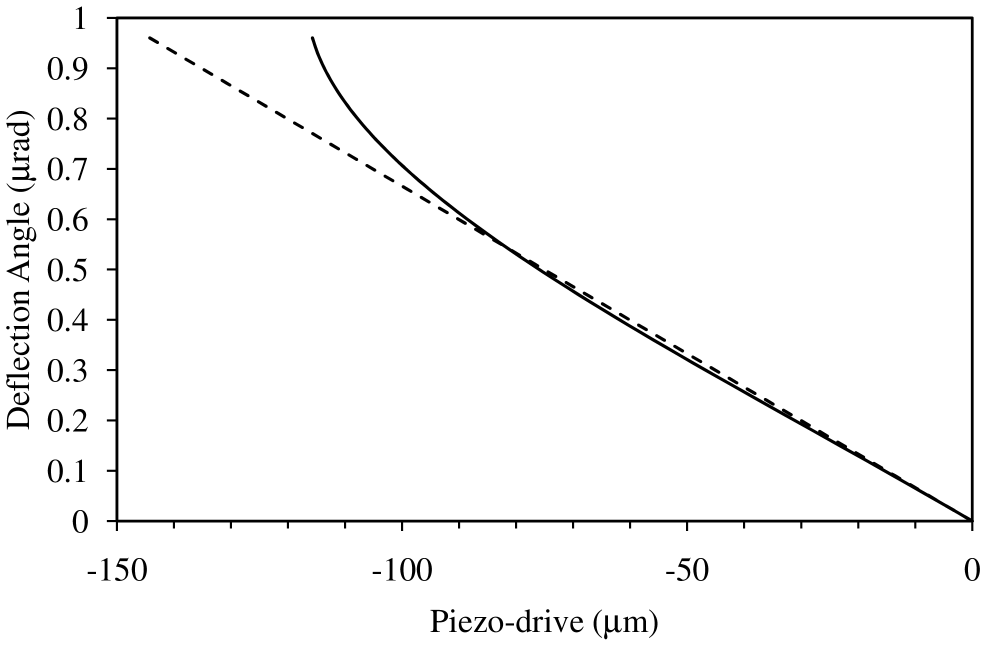
Figure 3: Calculated deflection angle versus the piezo-drive displacement in contact on extension ($L_{0}=235\,\mu$m, $R=10.11\,\mu$m, $\theta_{0}=-11^{\circ}$, and $\mu=0.375$). The solid curve is the non-linear calculation, and the dashed line is the linear calculation, which gives the tangent at first contact. Note that the total drive distance is rather large .

Figure 3 shows the deflection angle versus piezo-drive position calculated with the non-linear cantilever equations given above. In the displayed data, the photo-diode does not enter, and so the figure gives an indication of the non-linearity due to the cantilever alone. The linear result, the straight line, is just the tangent to the curve at first contact. One can see that the initial non-linear effect is for the angular deflection to increase at a slightly decreased rate (i.e. it dips below the tangent; the non-linear curve is initially concave down). Subsequently the angular deflection increases at an increasing rate and rises above the tangent, (the non-linear curve becomes concave up).

It should be emphasized that the drive distances in contact used in Fig. 3, although experimentally realizable, are on the order of 100 times larger than are used in a typical atomic force microscope force measurement. The point of the figure is to show what one might qualitatively expect from cantilever non-linearities in an experiment with large drive distances and a linear photo-diode.

The non-linearity may be characterised by the horizontal displacement of the tangent from the non-linear curve (the dashed line and the solid curve in Fig. 1) at a given voltage. Since the deduced change in piezo-drive position is the same as the change in tip position in contact, any such horizontal displacement appears directly as a change in separation. For the measured data in Fig. 1, at the end of the 300 nm piezo-drive range in contact, the difference between the actual piezo-drive and the piezo-drive position at which the linear tangent at contact gives the same voltage is 54 nm. For the calculated data for the non-linear cantilever used in Fig. 3, but over the same range of 300 nm, the difference is 1.2 nm.

One can conclude from these calculations that the non-linearity in the photo-diode is about 50 times greater than the non-linearity of the cantilever in this series of experiments.

III.4 Linear Cantilever, Non-Linear Photo-diode

The present series of experiments are likely representative of the norm, and the dominance of the photo-diode non-linearity over the cantilever non-linearity is likely the rule rather than the exception. Hence it is worthwhile to give explicitly the equations required to analyze atomic force microscope force data in the case of a non-linear photo-diode and a linear cantilever. These simplify the full analysis given earlier in this section. Essentially one takes the linear cantilever results from §II.2.3 and combines them with the non-linear data analysis results of §III.2.

For the linear cantilever, the lever arm is the constant $L_{2}=R\sqrt{2+2\cos\theta_{0}}$. Also, the deflection angle, force, and vertical tip position are all proportional to each other, Eqs (18)–(20),

$$\theta=E^{\mathrm{ext}}F_{z},\;x=D^{\mathrm{ext}}\theta\mbox{, and }z_{\mathrm{t}}=\theta/\alpha^{\mathrm{ext}}.$$ (68)

The superscript ‘ext’ ($\mu>0$), is replaced by ‘ret’ ($\mu<0$), or by ‘nc’ ($\mu=0$) in the respective regimes.

For the non-linear analysis of the measured data, the fit to the measured raw voltage is as in Eq. (47),

$$z_{\mathrm{pc}}^{\mathrm{ext}}(\tilde{V})=a_{0}+a_{1}^{\mathrm{ext}}\tilde{V}+a_{2}^{\mathrm{ext}}[\tilde{V}]^{2}+a_{3}^{\mathrm{ext}}[\tilde{V}]^{3}+\ldots$$ (69)

As in the linear case, the measured voltage is fitted to a straight line in the base-line region, Eq. (21),

$$\tilde{V}^{\mathrm{ext}}_{\mathrm{b}}(z_{\mathrm{p}})=\tilde{V}^{\mathrm{ext}}_{\mathrm{b}}+\tilde{\beta}^{\mathrm{ext}}_{\mathrm{b}}[z_{\mathrm{p}}-z_{\mathrm{pb}}].$$ (70)

Now the raw contact slope from the non-linear fit evaluated at the base-line voltage constant, $\tilde{V}^{\mathrm{ext}}_{\mathrm{b}}$ is given by Eq. (50),

$$\tilde{\beta}_{\mathrm{cb}}^{\mathrm{ext}} \equiv \left.\frac{\Delta\tilde{V}_{\mathrm{c}}^{\mathrm{ext}}}{\Delta z_{\mathrm{p}}}\right|_{\tilde{V}_{\mathrm{b}}^{\mathrm{ext}}}$$ (71)

$$= \frac{1}{a_{1}^{\mathrm{ext}}+2a_{2}^{\mathrm{ext}}\tilde{V}^{\mathrm{ext}}_{\mathrm{b}}+3a_{3}^{\mathrm{ext}}[\tilde{V}^{\mathrm{ext}}_{\mathrm{b}}]^{2}+\ldots}.$$

The rate of change of angle with tip position in the base-line region, the $\alpha_{\mathrm{b}}^{\mathrm{nc}}$ of Eq. (III.2), is the same as the $\alpha(0)$ of Eq. (20). The conversion factor for voltage to angle in the base-line region given by Eq. (III.2) is unchanged, $\gamma_{\mathrm{b}}^{\mathrm{ext}}=-\tilde{\beta}_{\mathrm{cb}}^{\mathrm{ext}}/\alpha_{\mathrm{b}}^{\mathrm{ext}}$.

The base-line angle and the base-line angle due to the surface force are unchanged from Eqs (54) and (55),

$$\theta_{\mathrm{b}}^{\mathrm{ext}}(z_{\mathrm{p}})=E^{\mathrm{nc}}F^{\mathrm{ext}}_{\mathrm{b}}+(\gamma_{\mathrm{b}}^{\mathrm{ext}})^{-1}\tilde{\beta}_{\mathrm{b}}^{\mathrm{ext}}[z_{\mathrm{p}}-z_{\mathrm{pb}}^{\mathrm{ext}}],$$ (72)

and

$$\theta_{\mathrm{bf}}^{\mathrm{ext}}(z_{\mathrm{p}})=E^{\mathrm{nc}}\left\{F^{\mathrm{ext}}_{\mathrm{b}}+F^{\mathrm{ext^{\prime}}}_{\mathrm{b}}[z_{\mathrm{p}}-z_{\mathrm{pb}}^{\mathrm{ext}}]\right\}.$$ (73)

The total effective angle in contact is formally the same as Eq. (58),

$$\tilde{\theta}_{\mathrm{tot,c}}^{\mathrm{ext}}(\tilde{V})=\theta_{0}+\theta_{\mathrm{c}}^{\mathrm{ext}}(\tilde{V})+\theta_{\mathrm{b}}^{\mathrm{ext}}(z_{\mathrm{pc}}(\tilde{V}))-\theta_{\mathrm{bf}}^{\mathrm{ext}}(z_{\mathrm{pc}}(\tilde{V})),$$ (74)

with the deflection angle now being linear in the tip position,

$$\theta_{\mathrm{c}}^{\mathrm{ext}}(\tilde{V})=\alpha^{\mathrm{ext}}\left[-z_{0}^{\mathrm{ext}}-z_{\mathrm{pc}}^{\mathrm{ext}}(\tilde{V})\right].$$ (75)

At a given measured datum $\{z_{\mathrm{p}},\tilde{V}\}$, in or out of contact, on extension, the deflection angle is formally the same as Eq. (59),

$$\theta(z_{\mathrm{p}},\tilde{V})=\tilde{\theta}_{\mathrm{tot}}(\tilde{V})-\theta_{0}-\theta_{\mathrm{b}}^{\mathrm{ext}}(z_{\mathrm{p}})+\theta_{\mathrm{bf}}^{\mathrm{ext}}(z_{\mathrm{p}}).$$ (76)

From this, the linear equations (68) give the force and also the separation, $h=z_{\mathrm{p}}+z_{\mathrm{t}}+z_{0}^{\mathrm{ext}}$.

The equations that give the constant that fixes the zero of separation are essentially unchanged from §III.2.1. One has the crude estimate of the piezo-drive position where the base-line intercepts the contact curve,

$$z_{\mathrm{pcb}}^{\mathrm{ext}}=a_{0}^{\mathrm{ext}}+a_{1}^{\mathrm{ext}}\tilde{V}^{\mathrm{ext}}_{\mathrm{b}}+a_{2}^{\mathrm{ext}}[\tilde{V}^{\mathrm{ext}}_{\mathrm{b}}]^{2}+a_{3}^{\mathrm{ext}}[\tilde{V}^{\mathrm{ext}}_{\mathrm{b}}]^{3}+\ldots,$$ (77)

and the refined version, Eq. (62),

$$z_{\mathrm{pcb}}^{\mathrm{ext,*}}=\frac{\tilde{\beta}_{\mathrm{cb}}^{\mathrm{ext}}z_{\mathrm{pcb}}^{\mathrm{ext}}-\tilde{\beta}_{\mathrm{b}}^{\mathrm{ext}}z_{\mathrm{pb}}^{\mathrm{ext}}}{\tilde{\beta}_{\mathrm{cb}}^{\mathrm{ext}}-\tilde{\beta}_{\mathrm{b}}^{\mathrm{ext}}}.$$ (78)

Equation (65) again follows, $\theta_{\mathrm{c}}^{\mathrm{ext}}(\tilde{V}^{*})=\theta_{\mathrm{bf}}^{\mathrm{ext}}(z_{\mathrm{pcb}}^{\mathrm{ext,*}})$, which in the present case can be rearranged as

$$z_{0}^{\mathrm{ext}}=-z_{\mathrm{pcb}}^{\mathrm{ext,*}}-[E^{\mathrm{nc}}/\alpha^{\mathrm{ext}}]\left\{F^{\mathrm{ext}}_{\mathrm{b}}+F^{\mathrm{ext^{\prime}}}_{\mathrm{b}}[z_{\mathrm{pcb}}^{\mathrm{ext,*}}-z_{\mathrm{pb}}^{\mathrm{ext}}]\right\}.$$ (79)

This exactly the same as given in §III.2.1, as one might expect since linear analysis suffices for the base-line.

IV Results

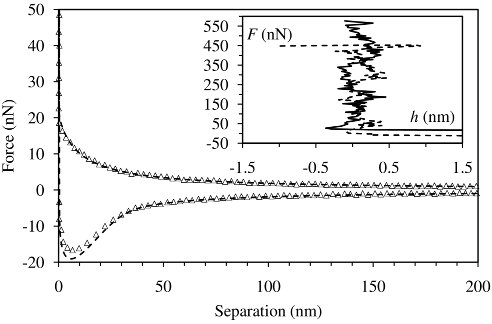
Figure 4: MeasuredZhu12 ; expt and calculated force versus separation for a drive velocity of $\dot{z}_{\mathrm{p}}=2\,\mu$m s^-1, viscosity $\eta=51.62\,$mPa s^-1, friction coefficient $\mu=0.35$, and cantilever spring constant $k_{0}=1.37\,$N/m. The symbols are the atomic force microscope data (upper is for extension, lower is for retraction), analyzed with the non-linear photo-diode, linear cantilever algorithm. The almost overlapping dashed curves are the calculated drainage force with a slip length of $b=3\,$nm and effective spring constant of $k_{\mathrm{eff}}=1.68\,$N/m. The right inset magnifies the measured data in contact (jagged solid curve is extension, jagged dashed curve is retraction).

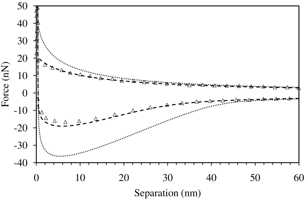
Figure 5: Magnification of previous figure at small separations. The symbols and dashed curves are as in the preceding figure, and the dotted curves are the calculated stick drainage force ($b=0\,$nm, $k_{\mathrm{eff}}=1.68\,$N/m).

Figure 4 shows the force versus separation data that corresponds to the raw measured data presented in Fig. 1. These and all of the experimental results presented in this section are analysed using the non-linear photo-diode, linear cantilever algorithm presented in the preceding subsection, unless explicitly stated otherwise. Four coefficients were used in each of the non-linear fits, $a_{0}$, $a_{1}$, $a_{2}$, and $a_{3}$ on each branch. The measurements in Fig. 4 were performed at low velocity, $\dot{z}_{\mathrm{p}}=2\,\mu$m s^-1, and so the magnitude of the drainage force is comparatively weak.

The figure includes the calculated drainage force, which is given by the Taylor equation with slip,

$$F=\frac{-6\pi\eta R^{2}\dot{h}}{h}f(h),$$ (80)

where the slip factor is Vinogradova95

$$f(h)=\frac{h}{3b}\left[\left(1+\frac{h}{6b}\right)\ln\left(1+\frac{6b}{h}\right)-1\right],$$ (81)

with $b$ being the slip length. The case $b=0$ (equivalently, $f(h)=1$) corresponds to stick boundary conditions.

A weak van der Waals force (Hamaker constant $1.3\times 10^{-21}\,$J m^-2) and short range repulsion (equilibrium separation 0.53 nm) derived from a Lennard-Jones 6-12 potential was included in order to calculate results in contact. These have no effect for separations greater than about 1 nm. Details of the algorithm used to calculate the drainage force may be found in Ref. Zhu11a, .

Comprehensive atomic force microscope measurements of the drainage force and of the slip length have been given in earlier work by the present authors, Zhu12 ; Zhu11a ; Zhu11b albeit with the linear analysis. The focus in the present work is not directly on the drainage force or the slip length, but rather on those aspects of the measurements where the non-linear analysis makes a difference.

Accordingly, one can briefly observe that the agreement between theory and measurement in Fig. 4 indicates the overall validity of the non-linear procedures developed here. The cantilever spring constant, $k_{0}=1.37\,$N/m, was obtained by fitting by eye the data and the calculated force at larger separations where the stick and slip theories overlap. In fact, at this velocity, $1.3\lesssim k_{0}\lesssim 1.6\,$N/m gave equally good fits. At the higher velocity $\dot{z}_{\mathrm{p}}=20\,\mu$m s^-1, $1.3\lesssim k_{0}\lesssim 1.5\,$N/m were acceptable, and at the still higher velocity $\dot{z}_{\mathrm{p}}=50\,\mu$m s^-1, $1.33\lesssim k_{0}\lesssim 1.42\,$N/m fitted the data. (The higher velocities gave larger drainage forces and the fits were more definitive. These cases are discussed in detail below.) Based on these fits, the value of the cantilever spring constant is taken to be $k_{0}=1.37\,$N/m, here and below. It is estimated that the value has been obtained with a precision of about $\pm 0.1\,$N/m. The effective spring constant corresponding to this is given by Eq. (34), $k_{\mathrm{eff}}=1.68\,$N/m. This effective spring constant should be used in the conventional linear analysis of the data, and in the theoretical calculations that use a simple spring model.

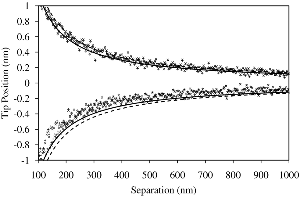
Figure 6: Fit for the spring constant, (data corresponding to Fig. 4). The vertical tip position, $z_{\mathrm{t}}=F/k_{\mathrm{eff}}$, is shown. The plus symbols are the non-linear analysis of the raw experimental data,Zhu12 ; expt the cross symbols are the original linear analysis of the same data,Zhu12 the solid curve is the position calculated from the stick drainage force ($b=0\,$nm, $k_{\mathrm{eff}}=1.68\,$N/m), and the dashed curve is the position calculated from the stick drainage force ($b=0\,$nm, $k_{\mathrm{eff}}=1.5\,$N/m).

Figure 6 shows the quality of the fit used to obtain the cantilever spring constant at the lowest drive velocity. It can be seen that a value of $k_{0}=1.37\,$N/m (equivalently, $k_{\mathrm{eff}}=1.68\,$N/m) slightly overestimates the magnitude of the deflection, more noticeably on the retraction branch, and that a slightly higher value would give a better fit in this case. Note that in order to reduce the fitting parameters from two to one, only the stick theory is used for the fit. (In any case the slip theory is virtually coincident at these large separations.) Also included is the original linear analysis of the same raw data,Zhu12 and the calculated stick drainage force that was used to fit a value of $k_{\mathrm{eff}}=1.5\,$N/m (equivalently, $k_{0}=1.23\,$N/m). First it may be observed that there is only a minor difference between the linearly and the non-linearly analyzed experimental data; the linear data slightly overestimates the magnitude of the deflection, and this effect increases as the magnitude of the force increases. Second, the value of the spring constant used originally is about 10% smaller than that fitted here. This gives a slightly better fit to the linearly analyzed extend data, but a worse fit on the retract curve, which was not taken into account in Ref. Zhu12, . At smaller separations than shown, the original and the present fits slightly improve, but in this region the slip length begins to have an effect and so it is better not to include it in the determination of the spring constant. Although the discrepancy in the spring constant is small (errors in other methods of cantilever calibration typically exceed 20%), it does lead to a large discrepancy in the fitted slip length and to qualitatively different behavior of the slip length with shear rate to that found here.

The overlap between the measured data and the slip calculations at short range in Figs 4 and 5 indicates that the correct slip length, $b=3\,$nm, has been obtained. The agreement is surprisingly good for the retract data, which was not analyzed in Refs Zhu12, ; Zhu11a, ; Zhu11b, , but which turns out to be very sensitive to the slip length. For example, the adhesive force, which is defined to be the minimum of the retract force, in Fig. 5 is measured to be $-16.6\,$nN, and it is calculated to be $-19.1\,$nN for $b=3\,$nm For the case of stick ($b=0\,$nm), it is calculated to be $-36.3\,$nN, which significantly overestimates the adhesion. The extend data is less sensitive to the slip length. For example, at $h=10\,$nm, the measured force is 10.5 nN, the calculated slip force for $b=3\,$nm is 10.1 nN, and the calculated stick force, $b=0\,$nm, is 13.2 nN. Based on this and the higher velocity results shown below, it is estimated that the slip length has been obtained with a precision of about $\pm 0.5\,$nm.

The linear analysis (not shown) of the measured extend data using the slope of the tangent at first contact gives 10.8 nN at $h=10\,$nm, and, using the slope of the tangent at final contact it gives $-16.5\,$nN for the adhesion. Hence the error due to the linear analysis is quite small at these points at this lowest velocity. It should be noted that the linear results were obtained using the effective spring constant $k_{\mathrm{eff}}=1.68\,$N/m rather than the cantilever spring constant, $k_{0}=1.37\,$N/m.

It is worth mentioning that the drainage measurements reported in Ref. Zhu12, found a low shear rate limiting slip length of $b_{0}=10\,$nm for the Si-Si case. This is significantly larger than is found here. In that investigation it was found that the slip theory progressively underestimated the measured force at small separations and overall it was a noticeably worse fit than found here. As mentioned above, the retract data was not included in the fit in Ref. Zhu12, . The most likely reason for the larger slip length and the degradation in the fit at small separations in Ref. Zhu12, compared to here is the difference in the value of the spring constant used: here $k_{\mathrm{eff}}=1.68\,$N/m, compared to $k_{\mathrm{eff}}=1.5\,$N/m in Ref. Zhu12, . A detailed discussion of how the linear analysis led to the contradiction between these earlier results and the present ones is given in the concluding section.

The friction coefficient was determined from the measured data in Fig. 4 by equalizing the extension and retraction calibration factors using the Guided Unbiased Estimate for a Single Solution algorithm, which is a rapid and well-used procedure for solving non-linear equations. A value of $\mu=0.38$ gave $\gamma^{\mathrm{ext}}_{\mathrm{cb}}=6357\,$V/rad and $\gamma^{\mathrm{ret}}_{\mathrm{cb}}=6359\,$V/rad. This is a little larger than the value determined by Stiernstedt et al.,Stiernstedt05 who obtained $\mu=$ 0.32–0.35 in four independent friction measurements (two probes, axial and lateral methods) for a silica probe on a silica substrate. In view of this a value of $\mu=0.35$ was used to analyse the data in Figs 4 and 5 and all of the following figures.

It was found that the value of the friction coefficient varied somewhat with the voltage at which $\gamma$ was evaluated. Obtaining $\mu$ by minimising $[\gamma^{\mathrm{ext}}(V;\mu)-\gamma^{\mathrm{ret}}(V;\mu)]^{2}$ over the contact region also gave a different value. In some case, particularly at higher drive velocities, unphysical values of $\mu$ were obtained. It was concluded that for these particular measurements in this high viscosity liquid the non-linear method could not be used to obtain the friction coefficient reliably. As is discussed further below, the most likely reason for the failure of this method of measuring the friction coefficient in the present case is the neglect of the variations in the drag force, which are most pronounced in contact.

Interestingly enough, the choice of the friction coefficient (and the choice of the fitting region) had almost no effect on the values of the measured non-contact forces. This is discussed further below, but in essence, the method of analyzing the non-contact data cancels the friction contribution whatever it may be.

The inset of Fig. 4 shows the force versus separation just prior to and in contact. Overall in contact the non-linear analysis gives a quite vertical curve that fluctuates about $h=0$ with apparent noise on the order of $\pm 0.5\,$nm. The verticality of the contact region of the data analysed with the non-linear algorithm is much better than that obtained with the linear analysis. As can be seen in the inset to Fig. 1, the linear analysis gives a systematic error in contact of 20–50 nm.

This noise in the non-linear data is not entirely random or unphysical (hence the word ‘apparent’) because any roughness of the surface gives rise to physical fluctuations in the apparent separation, as is discussed quantitatively shortly. In fact the presentation of the data in Fig. 4 exaggerates the apparent noise in the non-linear analysis. This is because the friction force is reversed on the retract branch compared to the extend branch, and so a given surface force $F$ corresponds to different contact positions on the substrate. Hence the disagreement between the extend and retract traces when presented in the form of force versus separation is entirely as one would expect.

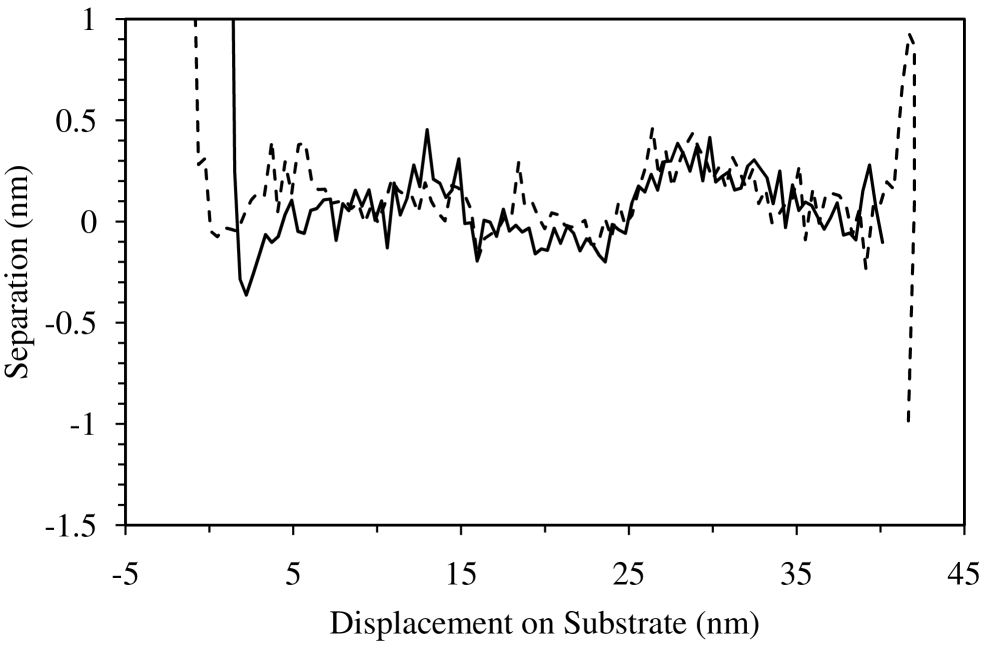
Figure 7: MeasuredZhu12 ; expt separation versus displacement on substrate in contact corresponding to Fig. 4. The solid curve is extension and the dashed curve is retraction.

One needs to compare the two branches at the same physical position on the substrate. The basis of the analysis of the tilted cantilever is that in contact the probe slides along the substrate in the axial direction of the cantilever, which is the origin of the friction force. The displacement from first contact of the probe on the substrate is simply $y=L_{2}\theta$. (Actually, the full expression is $y=S_{0}x-C_{0}L_{2}\theta=[S_{0}D^{\mathrm{ext/ret}}-C_{0}L_{2}]\theta$, but this is not used here.) This is used to plot the apparent separation, $h=z_{\mathrm{p}}+z_{\mathrm{t}}+z_{0}$, for extend and retract in Fig. 7. As in the preceding figure, the linear cantilever, non-linear photo-diode analysis was used to obtain $z_{\mathrm{t}}(\theta(\tilde{V},z_{\mathrm{p}}))$.

As mentioned in the text (c.f. the fourth paragraph of §II.2.5), the separation in contact measures the difference between changes in the piezo-drive position and changes in the tip position. It is positive when there is a protuberance on the substrate, and it is negative when there is a depression. That this is really a topographic map of the substrate can be seen by the high degree of correlation between the extend and the retract traces in Fig. 7. There are slight depressions, about 0.2 nm deep, at about $y=20\,$nm and $y=38\,$nm, and there is a protuberance, about 0.5 nm high, at about $y=30\,$nm. Where there is no correlation between the extend and retract traces, one can attribute the departure from zero to noise that is most likely connected with stick-slip motion of the probe on the substrate. One can conclude that the substrate is really quite smooth and, despite this noise, the method does give reliable topographic information with a resolution on the order of 0.1 nm.

It was found that $z_{0}^{\mathrm{ext}}=-1506.9\,$nm and that $z_{0}^{\mathrm{ret}}=-1507.8\,$nm. These differ by 1 nm, probably due to the reversal of the friction force on the two branches, which causes a displacement of the vertical position of the tip. This 1 nm difference appears to be essential to get the very precise overlap on the topographic plot. It is emphasized that the two values of $z_{0}$ were generated by the algorithm and no human judgement or adjustment was involved.

The rather pronounced feature in the start of the retract curve at about $y=42\,$nm in Fig. 7 is not a physical feature. It is an artefact of the reversal of direction of the piezo-drive on the change from extend to retract. This reversal begins at the start of the retract branch in this particular model of the atomic force microscope. At this turning point, the probe is essentially stuck at one contact position as the friction force reverses direction. During this turning phase the present analysis, which assumes that $F_{y}=-\mu F_{z}$, is not valid. For the same reason the negative separation of about $h\approx-0.5\,$nm just after first contact on extension is likely an artifact of the linear friction model.

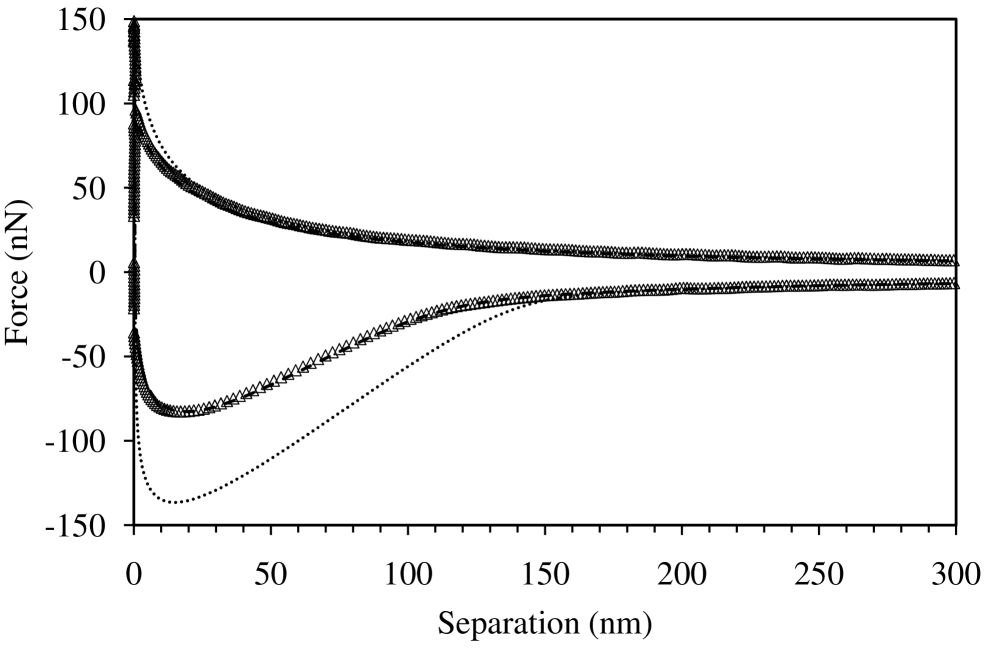
Figure 8: MeasuredZhu12 ; expt and calculated force versus separation for a drive velocity of $\dot{z}_{\mathrm{p}}=20\,\mu$m s^-1 and viscosity $\eta=52.25\,$mPa s^-1. The symbols are the atomic force microscope data (upper is for extension, lower is for retraction), analyzed with the non-linear photo-diode, linear cantilever algorithm with cantilever spring constant $k_{0}=1.37\,$N/m and with friction coefficient of $\mu=0.35$. The almost completely obscured dashed curves are the calculated drainage force with a slip length of $b=3\,$nm and $k_{\mathrm{eff}}=1.68\,$N/m. The dotted curves are the calculated drainage force for stick boundary conditions ($b=0\,$nm and $k_{\mathrm{eff}}=1.68\,$N/m).

Figure 8 shows the measured and calculated drainage force for a drive velocity of $\dot{z}_{\mathrm{p}}=20\,\mu\,$m s^-1, which is ten times the velocity of the preceding case. The viscosity $\eta=52.25\,$mPa s^-1 has slightly increased due to a temperature rise in the measurement cell. The cantilever spring constant was unchanged, $k_{0}=1.37\,$N/m. The calculated slip force (obscured dashed curves) was obtained with a simple spring model and the unchanged effective spring constant of $k_{\mathrm{eff}}=1.68\,$N/m and unchanged slip length $b=3\,$nm. The fact that an unchanged spring constant and slip length fit the measured data equally well at this high velocity as at the preceding low velocity indicates the reality of the values used, the validity of the mathematical form for the drainage force, and the reliability of the non-linear algorithm for the conversion of the raw measured signal into quantitative data.

The fact that the slip length is the same here as for the low velocity case (and for the higher velocity of $\dot{z}_{\mathrm{p}}=50\,\mu\,$m s^-1 presented below) suggests that the slip length is independent of the shear rate. This conclusion is reinforced by the fact that the slip theory with constant slip length fits the measured data over all separations (c.f. Figs 5 and 8), since the maximum shear rate of the drainage flow increases with decreasing separation. This contrasts with earlier work in which it was found that the slip theory increasingly underestimated the measured drainage force on extension as the separation approached zero.Zhu12a As was discussed above, such behavior occurs when the spring constant is underestimated, which was the case in Ref. Zhu12, from which series of measurements the raw data used here was taken. It is not known at this time whether or not a similar underestimate occurred in Ref. Zhu12a, . Accordingly, the claim that the slip length decreases with increasing shear rateZhu12a should be treated with caution pending a more refined analysis of that data.

The adhesion measured using the non-linear analysis is $-82.6\,$nN, and that calculated with the slip length $b=3\,$nm is $-82.6\,$nN. By way of comparison, the adhesion measured using the linear analysis and $k_{\mathrm{eff}}=1.68\,$N/m is $-80.8\,$nN (not shown), and that calculated with the stick theory $b=0\,$nm is $-136.6\,$nN. Note that it is essential to use the effective spring constant in order to get such reliable linear results.

The apparent separation in contact as a function of position on the substrate is shown in Fig. 9. There is a degree of correlation between the extend and retract traces, with a noticeable crater appearing in both at about $y=20\,$nm. The amount of noise is noticeably larger at this velocity of $\dot{z}_{\mathrm{p}}=20\,\mu$m s^-1 compared to the data in Fig. 7, which was obtained at a velocity of $\dot{z}_{\mathrm{p}}=2\,\mu$m s^-1. The physical origin of the increased noise is likely that more power is dissipated at the greater velocity. Two signatures of this change can be noticed. First is the reduced correlation between the extend and the retract traces. And second is that the amplitude of the fluctuations appear larger. The spatial wave length of the fluctuations is noticeably larger in Fig. 9 compared to Fig. 7. This indicates that the fluctuations are dynamic in nature, and that they probably have the same temporal frequency in both cases. This point explains why the low velocity data is more satisfactory in producing a topographic map of the surface: at low velocities the high frequency vibrations of the cantilever are averaged out in the time it takes to traverse a given spatial feature, whereas at high velocities the period of vibration and the spatial period are comparable and so they interfere with each other. One can conclude that the low velocity data gives more reliable results for the contact region than the high velocity case.

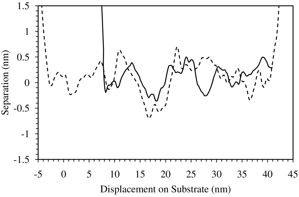
Figure 9: MeasuredZhu12 ; expt separation versus displacement on substrate in contact, (corresponding to preceding figure). The solid curve is extension and the dashed curve is retraction.

This last point is important. The friction coefficient used in the non-linear analysis in the high velocity case was $\mu=0.35$, which was taken from the low velocity data. (A non-linear fit in the contact region was still performed and used for the high velocity case.) This value of $\mu$ in the present case of $\dot{z}_{\mathrm{p}}=20\,\mu$m s^-1 gives calibration coefficients $\gamma^{\mathrm{ext}}_{\mathrm{cb}}=5660\,$V/rad and $\gamma^{\mathrm{ret}}_{\mathrm{cb}}=6425\,$V/rad. (In the analysis of the data, these values of $\gamma$ were used on each respective branch.) An unrealistically high value of $\mu=1.3$ is required to bring these into agreement at $\gamma_{\mathrm{cb}}=6250\,$V/rad. Although the required friction coefficient is unrealistically high, using it only changed the calibration coefficient by about 3%; the measured value of the adhesion remained unchanged at $-82.6\,$nN.

Besides the increased noise due to cantilever vibration, there are two further reasons why the high velocity data is unreliable in contact. First, in addition to the friction force, an axial drag force acts on the probe parallel to the substrate as it slides on the substrate. This axial drag force is not taken into account in the present analysis. It is exacerbated in high viscosity liquids and at high velocities. Second, the drag force normal to the cantilever, which is distinct from the drainage force, is not in fact constant as assumed here, but varies with load.Zhu11a ; Zhu11b (For determining the slip length, it is not necessary to use here a variable drag model because the cantilever is relatively stiff.)Zhu11a ; Zhu11b This variable drag effect increases with increasing viscosity, increasing velocity, and increasing force. Although for stiff cantilevers such as the present the variation in drag is relatively negligible in the non-contact region, in contact the variation is independent of the stiffness of the cantilever and so it can be expected to affect the present results. A simple calculation shows that here the axial drag force is several orders of magnitude smaller than the friction force. Hence it is most likely that it is the present neglect of the variable drag force in contact that makes the determination of the friction coefficient in the present series of measurements unreliable.

The question naturally arises that if the friction coefficient is unreliable for a given velocity, why can one use the non-linear contact fits at that velocity? There are two answers to this, one pragmatic and one reasoned. First, the evidence is that the fits are reliable and produce quantitative measured results, namely that the measured adhesion is insensitive to the value of the friction coefficient used in the analysis, and the measured force agrees quantitatively with the calculated force. Second, the non-linearity in the raw voltage measured in contact arises almost entirely from the photo-diode; the cantilever, including the friction, contributes to the linear part. The two drag forces just mentioned and neglected here also contribute to the linear part. Similar to the friction force, they reverse sign between extend and retract. The method of analyzing the non-contact data essentially cancels the friction contribution, and so it would also have canceled these drag contributions if they had been taken into account. This is the justification for using the friction coefficient measured at low velocities in combination with the non-linear fits applied at the current velocity.

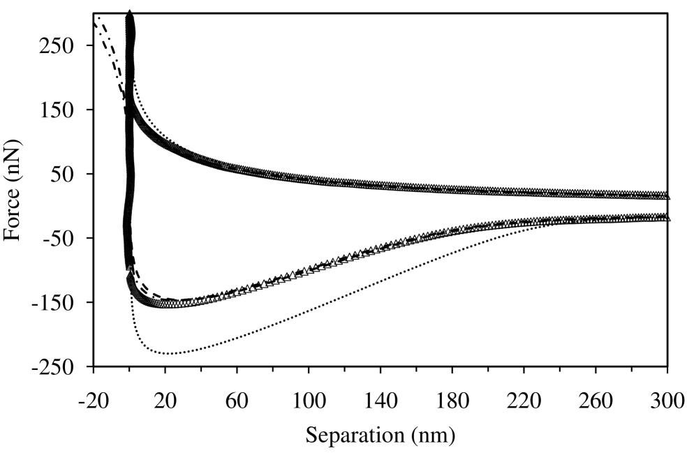
Figure 10: MeasuredZhu12 ; expt and calculated force versus separation for a drive velocity of $\dot{z}_{\mathrm{p}}=50\,\mu$m s^-1 and viscosity $\eta=52.25\,$mPa s^-1. The symbols are the atomic force microscope data (upper is for extension, lower is for retraction), analyzed with the non-linear photo-diode, linear cantilever algorithm with cantilever spring constant $k_{0}=1.37\,$N/m and with friction coefficient of $\mu=0.35$. The mainly obscured dashed curves are the calculated drainage force with a slip length of $b=3\,$nm and $k_{\mathrm{eff}}=1.68\,$N/m. The dotted curves are the calculated drainage force for stick boundary conditions ($b=0\,$nm and $k_{\mathrm{eff}}=1.68\,$N/m). The obscured dash-dotted curves are measured data analyzed with the conventional linear approach using $k_{\mathrm{eff}}=1.68\,$N/m, with the zero of separation established as described in §II.2.5.

Figure 10 shows the measured and calculated force for a drive velocity of $\dot{z}_{\mathrm{p}}=50\,\mu$m s^-1. The measured data are analyzed with the non-linear algorithm of §III.4 (symbols), and with the linear algorithm of §II.2 using the tangent at first (extension) or last (retraction) contact (dash-dotted curves). The cantilever spring constant, $k_{0}=1.37\,$N/m, slip length, $b=3\,$nm, and friction coefficient, $\mu=0.35$, have been fixed at the values determined in the low velocity case, $\dot{z}_{\mathrm{p}}=2\,\mu$m s^-1.

With this value of $\mu$, in the present case of $\dot{z}_{\mathrm{p}}=50\,\mu$m s^-1 the calibration coefficients are $\gamma^{\mathrm{ext}}_{\mathrm{cb}}=6263\,$V/rad and $\gamma^{\mathrm{ret}}_{\mathrm{cb}}=6416\,$V/rad. A value of $\mu=0.57$ gives $\gamma^{\mathrm{ext}}_{\mathrm{cb}}=6361\,$V/rad and $\gamma^{\mathrm{ret}}_{\mathrm{cb}}=6365\,$V/rad.

The adhesion measured using the non-linear analysis is $-153\,$nN, that measured using the linear analysis is $-147\,$nN , that calculated with the slip length $b=3\,$nm is $-147\,$nN, and that calculated with the stick theory $b=0\,$nm is $-230\,$nN.

In the case of the linear analysis, the zero of separation was established as described in §II.2.5. This removes any human intervention or bias, which can be a problem in the conventional linear analysis where each curve is shifted horizontally so that it gives $h=0$ at what appears by eye to be first or last contact. In fact, in the absence of the non-linear result it would have been difficult to establish contact with any confidence in this case due to the smooth and continuous nature of the forces and the lack of verticality in contact in the linearly analyzed data. These results with negative gradient and negative separation for the linear analysis in contact is a significant failing of the approach.

The verticality of the linear analysis in contact for forces $F_{z}\in[-150\,$nN,$150\,$nN$]$, suggests that the photo-diode is linear in this range. Since the non-contact forces also lie in this range, one can understand why the linear analysis with effective spring constant works in this high velocity case.

It can be noted in Fig. 10 that the maximum magnitude of the drainage forces out of contact are about on the limit of photo-diode linearity. At higher velocities they will enter the non-linear regime, and so one would expect the linear analysis to become progressively less reliable as the velocity is increased.

It can also be seen that on the extension branch, in this figure and in the preceding figures, there is no overlap between the contact voltages and the non-contact voltages. However, the retraction branch in contact encompasses all of the non-contact voltages. Whereas extrapolation of the contact fit is required on extension, only interpolation is required on retraction branch.

There is a noticeable discontinuity in the non-linear measured data at final contact on retraction, and at first contact on extension (obscured). This is an artefact of the linear friction model, which is zero out of contact, and jumps discontinuously to a non-zero value in contact. Whenever the load is non-zero at such a point, the friction force is discontinuous and it gives rise to a discontinuity in the analyzed data.

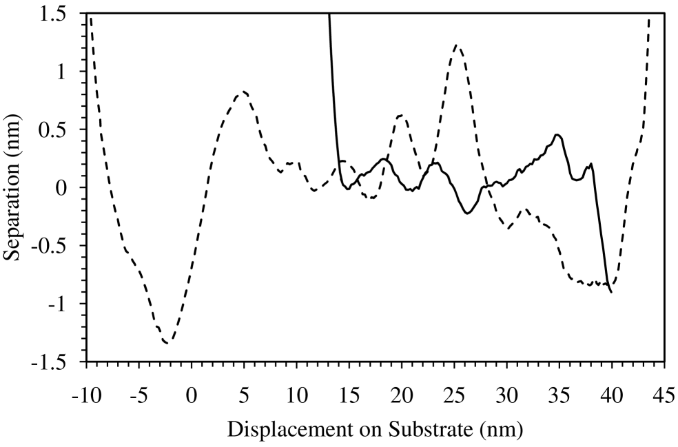
Figure 11: MeasuredZhu12 ; expt separation versus displacement on substrate in contact corresponding to preceding figure. The solid curve is extension and the dashed curve is retraction.

Figure 11 shows the apparent separation versus contact position on the substrate at this highest velocity. In this case it is difficult to see a correlation between the extend and the retract traces. The spatial wave length of the noise is large, as one might expect of temporal vibrations at this high speed, and they appear to dominate any topographic features. The pronounced feature at the start of the retract trace at $y=45\,$nm is an artefact of the turn point and the inapplicability of the linear friction model there. Likewise, the pronounced feature near final contact, $y\lesssim 0\,$nm on retraction, which can also be seen in Fig. 9, is also likely an artifact of the linear friction model, $F_{y}=-\mu F_{z}$. In this region on retraction just prior to pull-off there is a pronounced adhesion and $F_{z}<0$. The linear friction model is only valid, if at all, for positive loads. In this context it is worth mentioning that there is a modified form of Amontons law, $F_{y}=\mu[F_{z}-A]$, where $A$ is the adhesion.Derjaguin94 There is some experimental support for this,Stiernstedt05 ; Feiler00 but it has not been explored in the present investigation.

In §II.2.7 a method of extracting the drag force was given, which was characterized by an effective length that was expected to be somewhat less than the length of the cantilever. The validity of the procedure could be checked from the extent to which the effective length was independent of the drive velocity. For velocities $\dot{z}=$ 2, 20, 50, and 80$\,\mu$m s^-1, it was found that $L_{\mathrm{eff}}=$ 83.2, 92.9, 77.7, and 88.1$\,\mu$m, respectively. These are remarkably consistent. There was some dependence on the choice of the base-line region. In the worst case, $\dot{z}=$ 2$\,\mu$m s^-1, reducing the range of the base-line by a factor of almost 3, from 1.83$\,\mu$m to 0.65$\,\mu$m increased the drag length by about 20%.

V Conclusion

This paper has investigated the causes of non-linearity in the contact region of atomic force microscope measurements of surface forces, and has developed an algorithm for analyzing data when such curved compliance occurs. Two sources of non-linearity —large cantilever deflection and photo-diode response— were identified and investigated. It was concluded that in a typical case the non-linear photo-diode response was the dominant contribution to the observed non-linearity in contact.

A relatively simple algorithm for analyzing raw experimental data was developed. The numerical algorithm invoked a non-linear polynomial fit to the measured voltage in the contact region, and was found easy to implement with a spread sheet.

The first advantage of the algorithm is that it eliminates the ambiguity in the choice of the contact slope (constant compliance factor) that occurs when one has a curved contact region. Even when, or, more precisely, especially when, the non-contact forces are in the linear response regime, one still needs this calibration factor to convert the measured photo-diode voltage to force and separation. It significantly improves the quantitative reliability of the atomic force microscope to have an algorithm that gives it correctly and unambiguously.

A second advantage is that the algorithm eliminates non-physical behavior of the analysed data in the contact region that is an artifact of the linear analysis. The results show that the non-linear analysis yields reliable topographic data in the contact region with sub-nanometer accuracy.

The complete non-linear analysis of cantilever deflection is useful even though it turns out that in this instance it is not required in full. The full analysis was simplified to the linear case but it still included the effects of cantilever tilt, friction in contact, and torque due to the extended probe. These are often neglected in the conventional analysis but they are required for accurate and reliable analysis of raw experimental data. In particular, a third feature of the analysis is that it gives the relationship between the intrinsic cantilever spring constant, which is a material property of the cantilever and which is the quantity usually measured by calibration procedures, and the effective spring constant, which is the quantity required to convert the measured vertical cantilever deflection to a surface force. The difference between these two can typically be 10% or more, and using the wrong one can lead to unacceptable errors in the measured surface force.

A fourth feature of the data analysis algorithm is the accounting of measurement artifacts such as virtual deflection, thermal drift, cantilever drag, and long-range surface force asymptotes. The proper treatment and elimination of these is automated using relatively straight forward linear corrections.

A fifth innovation is an automated numerical procedure for fixing the zero of separation. The advantage of this is that it eliminates the ambiguity that exists in the conventional analysis and it avoids human intervention and bias. An unambiguous and precise definition of zero can be essential when finer details of surface forces in the non-contact region are required.

V.0.1 Reconciliation with Earlier Results

The non-linear algorithm was applied to measured raw atomic force microscope data that had previously been analyzed using the conventional linear approach. The validity of non-linearly analyzed data was confirmed by the quantitative agreement with the calculated drainage force over a range of velocities.Zhu12 In particular, quantitative agreement occurred for the measured drainage adhesion, which had not previously been analyzed in detail.

Some effort was made to test the conventional linear analysis when the data showed a non-linear contact region (curved compliance). It was found that provided the correct effective spring constant was used in the linear analysis, the measured pre-contact forces agreed with the non-linearly analyzed data. Obviously, if the intrinsic cantilever spring constant was used instead, as is often the case in conventional analysis, the non-contact force was underestimated by about 10%. Also, in order to get agreement, the zero of separation had to be established using the (linear) algorithm given here.

The slip length obtained on the basis of the present non-linear analysis was 3 nm and it was found to be independent of shear rate. In the previous work where the data was analyzed with the linear algorithm,Zhu12 the slip length was found to decrease with increasing shear rate, and to have a low shear rate limiting value of 10 nm. These qualitative and quantitative discrepancies were attributed directly to an underestimate of the cantilever spring constant in the previous work,Zhu12 which is a consequence of the linear analysis used there.

In the light of the present results and analysis one can explain the reasons for the two major discrepancies between the present results and the earlier results: the much larger slip length, and the decrease in slip length with increasing shear rate found earlier. The earlier analysis used as the calibration factor (the conversion factor between photodiode voltage and cantilever deflection) the gradient of the contact extension curve measured at first contact. This corresponds to the lowest extension contact force but the greatest extension non-contact drainage force. Because the contact curve is concave down due to the non-linearity in the photodiode response (see Fig. 1), this value of the calibration factor underestimates the actual response in the non-contact region. Hence, the deflection of the cantilever (voltage divided by calibration factor) was overestimated in the earlier work. Hence the effective spring constant used in the theory to fit this measured deflection at large separations was underestimated. (This explains the earlier $k_{\mathrm{eff}}=1.5\,$N/m,Zhu12 compared to the present $k_{\mathrm{eff}}=1.68\,$N/m.) However, using too soft a cantilever in the theoretical calculations of the drainage force overestimates the curvature (rate of increase with separation) in the calculated deflection compared to the actual curvature at intermediate separations. For the given spring constant, the only way to reduce the theoretical force so that it agrees with the calculated force at intermediate separations is too increase the slip length, which causes it to be overestimated. (This explains the earlier $b_{0}=10\,$nm,Zhu12 compared to the present $b=3\,$nm.) However, at small separations, where the pre-contact voltage is close to the first contact voltage, the calibration factor that was used earlier is relatively accurate, and the artificial compensation factors (too small a spring constant, too large a slip length) that worked at large and intermediate separations are not required at small separations. Hence for the given spring constant, the overestimated slip length that fitted at intermediate separations needs to be reduced at small separations to fit theory to the analysed measured data. Since the shear rate increases with decreasing separation, this explains the discrepancy between the earlier conclusion that the slip length decreases with increasing shear rate,Zhu12 and the present conclusion that it is constant. This chain of reasoning likely applies as well to other measurements.Zhu11a ; Zhu11b ; Zhu12a

Besides substantially improving the reliability of the non-contact results, the non-linear analysis gives useable results in the contact region. It was shown that reliable topographic information could be extracted from the contact data with sub-nanometer resolution. The data was most reliable at low drive velocities.

A second material property obtainable in contact was the friction coefficient. The value obtained here at the lowest velocity, $\mu=0.35$, was consistent with values previously obtained for Si–Si.Stiernstedt05 However, the results were sensitive to the point in contact at which it was measured, or else to the range chosen if it was averaged in the contact region. Also, they deteriorated badly as the drive velocity was increased. It was concluded that the results were being effected by variable drag,Zhu11a ; Zhu11b which was neglected here. This effect is exacerbated in high viscosity liquids and at high drive velocities. Fortunately, it was shown that the pre-contact forces in the analyzed experimental data were not sensitive to the value of the friction coefficient. However, to improve the performance in high viscosity liquids of this method for measuring friction, variable drag will have to be accounted for.

- (1) Binnig, G., Quate, C., and Gerber, Ch. (1986), Phys. Rev. Lett. 56, 930.
- (2) Marti, O., Elings, V., Haugan, M., Bracker, C. E., Schneir, J., Drake, B., Gould, S. A. C., Gurley, J., Hellemans, L., Shaw, K., Weisenhorn, A. L., Zasadzinski, J., and Hansma, P. K. (1988), J. Microscopy 152, 803.
- (3) Meyer, G. and Amer, N. M. (1988), Appl. Phys. Lett. 53, 1045.
- (4) Ducker, W. A. and Senden T. J. (1991), Nature 353, 239.
- (5) In the atomic force microscope modeled here, the piezo-drive is connected to the cantilever holder and is above the substrate. In extension the velocity of the piezo-drive is negative, , and in contact the movement of the cantilever tip is equal and opposite to that of the piezo-drive, . In other models of the atomic force microscope, it is the substrate that is connected to the piezo-drive, so that on extension and in contact . These other models may be analysed with the formulae given in this paper by negating the piezo-drive position in the raw data, .
- (6) Zhu, L., Attard, P., and Neto, C. (2012), Langmuir, 28, 7768.
- (7) The atomic force microscope was an Asylum Research Instruments, MFP-3D. The probe was a silicon colloid, m, the tilt angle was , the substrate was a silicon wafer, and the liquid was di-n-octylphthalate (DOPC, viscosity mPa s). A rectangular cantilever (NSC12/tipless (4c), Mikromasch, Estonia) of length m was used. The measured data are taken from the same series of experiments as those reported in Ref. Zhu12, , which may be consulted for further details.
- (8) Southwell, R. V. (1936), An Introduction to the Theory of Elasticity, (Oxford, London).
- (9) Higgins, J., Proksch, R., Sader, J. E., Polcik, M., McEndoo, S., Cleveland, J. P., and Jarvis, S. P. (2006), Rev. Sci. Instrum. 77, 013701 .
- (10) Attard, P., Pettersson, T., and Rutland, M. W. (2006), Rev. Sci. Instrum. 77, 116110.
- (11) Craig, V. S. J. and Neto, C. (2001), Langmuir 17, 6018.
- (12) Zhu, L., Attard, P., and Neto, C. (2011), Langmuir, 27, 6701.
- (13) Zhu, L., Attard, P., and Neto, C. (2011), Langmuir, 27, 6712.
- (14) Attard, P., Schulz, J., and Rutland, M. W. (1998), Rev. Sci. Instrum. 69, 3852.
- (15) Attard, P., Carambassis, A., and Rutland, M. W. (1999), Langmuir 15, 553.
- (16) Stiernstedt, J., Rutland, M. W., and Attard, P. (2005), Rev. Sci. Instrum. 76, 083710. Erratum, (2006) Rev. Sci. Instrum. 77, 019901.
- (17) Feiler, A., Larson, I., Jenkins, P., and Attard, P. (2000), Langmuir 16, 10269.
- (18) Vinogradova, O. I. (1995), Langmuir, 11, 2213.
- (19) Zhu, L., Neto, C. and Attard, P. (2012), Langmuir, 28, 3465.
- (20) Derjaguin, B. V. and Toporov, Y. P. (1994), Prog. Surf. Sci. 45, 317.