The black hole - bulge mass relation of Active Galactic Nuclei in the Extended $Chandra$ Deep Field - South Survey

Abstract

We present results from a study to determine whether relations, established in the local Universe, between the mass of supermassive black holes (SMBHs) and their host galaxies are in place at higher redshifts. We identify a well-constructed sample of 18 X-ray-selected, broad-line Active Galactic Nuclei (AGN) in the Extended $Chandra$ Deep Field South - Survey with $0.5<z<1.2$. This redshift range is chosen to ensure that HST imaging is available with at least two filters that bracket the 4000 Å  break thus providing reliable stellar mass estimates of the host galaxy by accounting for both young and old stellar populations. We compute single-epoch, virial black hole masses from optical spectra using the broad MgII emission line. For essentially all galaxies in our sample, their total stellar mass content agrees remarkably well, given their BH masses, with local relations of inactive galaxies and active SMBHs. We further decompose the total stellar mass into bulge and disk components separately with full knowledge of the HST point-spread-function. We find that $\sim 80$% of the sample is consistent with the local $M_{\mathrm{BH}}-M_{*,\mathrm{Bulge}}\,$relation even with $72\%$ of the host galaxies showing the presence of a disk. In particular, bulge dominated hosts are more aligned with the local relation than those with prominent disks. We further discuss the possible physical mechanisms that are capable building up the stellar mass of the bulge from an extended disk of stars over the subsequent eight Gyrs.

1. Introduction

A determination of the physical mechanisms through which supermassive black holes are built up at the centers of galaxies have been one of the key issues in astrophysics (see Kormendy & Richstone, 1995). Such processes are thought to further provide a link black hole growth and the formation of the bulges of their host galaxies based on both observations and theory. Correlations between the mass of the central black hole and absolute magnitude (Magorrian et al., 1998; Marconi & Hunt, 2003; Häring & Rix, 2004), and/or stellar velocity dispersion (Gebhardt et al., 2000; Merritt & Ferrarese, 2001) of the spheroidal component indicate that the mass ratio between a SMBH and its bulge is constant over a wide dynamic range in mass (e.g. $M_{BH}/M_{Bulge}$= 0.0014; Häring & Rix (2004); hereafter $M_{BH}-M_{Bulge}$ relation). We will refer to this relation as the local relation.

Over the past years, several studies have addressed whether there is an evolution of the mass relations between the central black hole and its host galaxy. Such studies must rely upon galaxies with accreting SMBHs (i.e., Active Galactic Nuclei; AGN) since the region of influence surrounding black holes cannot be resolved at higher redshifts. While those hidden by obscuration (i.e., type 2 AGNs) give a rather clean view of their host galaxy, unobscured (type 1) AGN are the only systems for which black hole masses can be measured. Although, an estimate of the mass of the host bulge is challenging due to the glare of a luminous AGN that only gets more difficult at high redshift. Fortunately, optical imaging from space with HST can be used to disentangle the light between an AGN and its host galaxy (e.g., Sánchez et al., 2004; Jahnke et al., 2004, 2009; Bennert et al., 2011b; Cisternas et al., 2011) due to the high spatial resolution and well understood point spread function. Alternatively, it is also possible to measure the stellar velocity dispersion from optical spectra for less luminous AGNs (Woo et al., 2008); this method requires high signal-to-noise spectra that limits its application to high redshift AGNs.

Even if the host galaxy is resolved only limited spectral coverage is usually available to estimate stellar masses. Single-band studies are therefore restricted to the black hole mass - luminosity relation or have to make assumptions on the mass-to-light ratio of the host galaxy (see Peng et al., 2006a, b; Decarli et al., 2010a, b). Merloni et al. (2010) implemented a new approach to measure the stellar mass content of AGN host galaxies through template fitting of the broad-band photometric spectral energy distribution (Brusa et al., 2009; Xue et al., 2010). With this approach, Merloni et al. (2010) estimate the total stellar mass content which provides only an upper limit to the bulge mass. Bennert et al. (2011) take a significant step forward by using the multi-band HST data available in the GOODS (Giavalisco et al., 2004) fields to decompose the AGN and host galaxy light including a bulge component tractable through multiple filter bandpasses. Unfortunately, the sample is selected to be a redshifts ($1<z<2$) for which the optical imaging falls below the rest-frame 4000 Å  break. Surprisingly, the aforementioned studies find elevated black hole masses as compared to either the bulge component (Woo et al., 2008; Bennert et al., 2011b) or total (Merloni et al., 2010) stellar mass of their host galaxy. Recently, Jahnke et al. (2009) and Cisternas et al. (2011) report that the mass ratio between the black hole and the total stellar mass of its host galaxy is similar to local values possibly indication of an undermassive bulge.

Even with the considerable effort achieved to date, there are several challenges that need to be met in order to accurately determine the evolution of the $M_{\mathrm{BH}}-M_{*,\mathrm{Bulge}}\,$at higher redshift. First, the decomposition of optical light is more difficult due to the strong surface brightness dimming of the host galaxy as compared to the AGN. To mitigate this effect, high resolution imaging with high signal-to- noise is needed to adequately resolve the host galaxy especially for bright AGN. Equally important, at least, one rest-frame optical color and a luminosity is needed to constrain the stellar mass content of the host galaxy (Bell et al., 2003). A color that covers the 4000 Å break provides a good estimator on the underlying stellar mass-to-light ratio. It is worth highlighting that the 4000 Å  break moves out of the optical filter bands at $z>1.2$ thus requiring deep high-resolution NIR imaging. Furthermore, due to the limited physical resolution at high redshift and the fact that galaxies become more compact, it may be challenging to classify galaxies morphologically such as distinguishing between disturbed and undisturbed hosts.

A determination of the $M_{\mathrm{BH}}-M_{*,\mathrm{Bulge}}\,$ relation using AGN samples, also requires an assessment of the possible biases originating from selection of AGN (see Salviander et al., 2007; Lauer et al., 2007). While quiescent galaxies are selected by their magnitude or luminosity, active galaxies (e.g., unobscured, broad-line AGN) are often selected by their optical nuclear luminosity or magnitude. The bias introduced by the luminosity (i.e., mass) limit will have a stronger effect at the high mass end of the black hole mass function which is strongly decreasing. Offsets from the local $M_{\mathrm{BH}}-M_{*,\mathrm{Bulge}}\,$relation seen in samples of luminous AGN with massive BHs (e.g., Merloni et al., 2010; Bennert et al., 2011b; Peng et al., 2006a, b) may be explained by such a bias. Therefore, a sample selected at lower luminosities that fall well below the knee of the black hole mass function should be less impacted by such a bias.

In this study, we determine the $M_{\mathrm{BH}}-M_{*,\mathrm{Total}}\,$and $M_{\mathrm{BH}}-M_{*,\mathrm{Bulge}}\,$relations at $0.5<z<1.2$ using a sample of 18 X-ray selected broad-line AGN (BLAGN) from the Extended $Chandra$ Deep Field - South Survey. Based on HST/ACS imaging from GEMS (Rix et al., 2004) and GOODS (Giavalisco et al., 2004), we measure the stellar mass content of their host galaxies including the bulge component. We specifically focus on this redshift range so that there is at least one HST band above and below the 4000 Å break thus providing a rest-frame color required for accurate conversion of light to mass. Black hole masses are determined using single epoch virial mass estimation based on the MgII emission line. In Section 2, we describe our sample. In Section 3, we describe our analysis of the HST/ACS data that involves the image decomposition of the total light into AGN, bulge and disk decomposition, and stellar mass estimation. Black hole masses are fully detailed in Section 4. Section 5 and 6 presents the results including a discussion of the relations between the mass of the SMBH and their total/bulge stellar mass. Finally, in Section 7 we give a summary of the results. Throughout this paper we assume a flat cosmology with $H_{0}=70~{}\mathrm{km\,s}^{-1}\,\mathrm{Mpc}^{-1}$, $\Omega_{M}=0.3$ and $\Omega_{\Lambda}=0.7$.

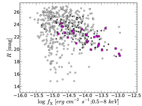
Figure 1.— Optical $R$-band magnitude versus broad-band X-ray flux (0.5-8 keV; units of ergs cm² s^-1) for all X-ray sources from Lehmer et al. 2005 (grey circles). All sources classified as BLAGN have been marked with a black dot. Our final sample selection is shown as magenta solid squares. Objects falling below the typical relation for type I AGNs are the obscured (type II) AGNs (see Figure 5 of Silverman et al., 2010).

2. AGN Sample

Currently, broad-line (type 1) AGNs provide the only means to establish the relation between BH mass and galaxy mass beyond the local universe. This is due to the fact that BH mass measurements rely upon a determination of the velocity widths of gas in the vicinity of the BH as provided by broad emission lines (e.g., Kaspi et al., 2000; Vestergaard & Peterson, 2006). High-resolution imaging (best if taken from space) can then be used to detect the extended emission from the underlying host galaxy. There have been numerous studies of the host galaxies of type 1 AGNs using such techniques (e.g., Jahnke et al., 2004, 2009; Sánchez et al., 2004; Bennert et al., 2011b; Cisternas et al., 2011).

We aim to take advantage of type 1 AGNs that are found in X-ray surveys, such as the $Chandra$ Deep Field South - Survey, that reach faint depths. These X-ray sources are likely to have a wide range in their optical properties that includes those of lower luminosity both missed in optically-selected samples such as SDSS, and more favorable for the study of their host galaxy. There are numerous papers on the host galaxies of X-ray selected AGN that may be of interest to the reader (e.g., Grogin et al., 2005; Pierce et al., 2007; Ammons et al., 2009; Silverman et al., 2008).

Here, we specifically select type 1 AGNs from the compilation of Silverman et al. (2010) that provide spectroscopic redshifts and classification of X-ray sources in the the Extended $Chandra$ Deep Field South - Survey (Lehmer et al., 2005). These are objects with at least one broad emission line having a FWHM greater than 2000 km s^-1. We further require that an available spectrum has a good enough quality to perform our emission line fitting procedure to estimate virial black hole masses.

We then demand that each type 1 AGN has been observed by HST. The ECDFS is covered by the GEMS (Rix et al., 2004) and GOODS (Giavalisco et al., 2004) surveys in the central area. GEMS consists of imaging in two optical HST filters (ACS F606W and F850LP) while GOODS has four filters (ACS F435W, F606W, F775W and F850LP). Unfortunately, some sources are located on the outskirts of the ECDFS and therefore no HST coverage is available. Even though, extensive ground based data is available of the full ECDFS area from various observing campaigns (e.g., MUSYC survey; Cardamone et al., 2010), we choose to avoid any biases that may appear due to the inclusion low resolution data. We further stress that is essential to have at least two filters that bracket the 4000 Å break in the rest-frame of the host galaxy for accurate estimation of the mass-to-light ratio and the stellar mass (see the following section). To do so, we elect to restrict the type 1 AGN sample to $0.5<z<1.2$ that allows us to determine accurate rest-frame B-V colors for the entire sample. In addition, we apply the same selection to the deeper 2Msec catalog (Luo et al. 2008) and identify one additional source. Our final sample consists of 18 type 1 AGN with half falling in the GOODS area and the other half within the GEMS field. In Figure 1, we show the distribution of X-ray flux and R-band optical magnitude of $Chandra$ sources and highlight those within our type 1 AGN sample. It is apparent that the sample spans about two dex in both X-ray flux or luminosity, and optical brightness. The final sample covers the full region of the $f_{X}-R$ plane as the overall BLAGN sample.

Table 1Sample: Target List and results from the analysis. The different columns show (1) Object ID taken from the Lehmer et al., (2),(3) Ra DEC coordinates, (4) redshift, (5) absolute V-bband magnitude,(6) rest-frame U-V color of the host galaxy ,(7) Sersic Index from single Sersic fit,(8) half-light radius of the bulge and disk in arcsec in F850LP (9) total stellar mass, (10) bulge-to-total luminosity ratio, (11) FWHM of the MgII emission line, (12) continuum luminosity at 3000Å, (13) BH mass, (14) Eddington Ratio, (15) nuclear-to-host ratio in F850LP, (16) survey field:GEMS [1] & GOODS [2]

Source ID	RA	Dec	$z$	$M_{V}^{\rm{host}}$	$U-V$	Sersic	$r_{\mathrm{bulge}}/r_{\mathrm{disk}}$	$M_{\rm{tot}}$ [$M_{\odot}$]	B/T	FWHM	$L_{3000}$	log $M_{\mathrm{BH}}\,$	$\epsilon$	N/H	Field
$[1]$	[2]	[3]	[4]	[5]	[6]	Index [7]	[8]	[9]	[10]	[11]	[12]	[13]	[14]	[15]	[16]
158	52.942418	-27.952407	0.717	-21.70	0.78	4.0	0.83/-	10.66	1.00	3.24	43.22	7.08	0.07	0.05	[1]
170	52.949839	-27.845910	1.065	-20.33	0.04	2.2	0.07/0.12	9.80	0.50	3.12	42.85	6.98	0.05	0.11	[1]
250	53.001530	-27.722073	1.037	-21.20	0.84	7.7	0.13/-	10.19	1.00	4.12	44.01	7.64	0.09	1.00	[2]
271	53.125255	-27.756535	0.960	-21.08	0.76	1.4	-/-	10.49	0.23	2.72	43.86	7.26	0.19	0.54	[2]
273	53.016951	-27.623708	0.970	-20.39	0.96	4.3	0.22/-	10.29	1.00	6.96	43.84	8.13	0.03	1.22	[1]
305	53.036121	-27.792822	0.544	-22.47	0.58	4.0	0.77/-	11.01	1.00	5.80	44.98	8.52	0.14	1.51	[2]
333	53.057789	-27.602162	1.044	-21.06	0.41	1.1	0.08/0.14	10.33	0.35	6.40	43.29	7.80	0.02	0.19	[1]
339	53.062421	-27.857514	0.675	-22.00	1.04	5.5	0.32/-	10.96	1.00	9.81	42.60	7.74	0.00	¡0.03	[2]
348	53.071454	-27.717531	0.569	-21.51	0.72	1.2	0.21/0.24	10.55	0.40	5.82	43.91	7.78	0.04	0.08	[2]
375	53.110383	-27.676530	1.031	-22.41	-0.12	1.1	-/-	10.55	0.10	3.02	45.18	7.92	0.63	3.14	[2]
379	53.112521	-27.684732	0.737	-22.49	0.02	2.4	-/-	10.66	0.32	10.30	45.05	9.04	0.05	3.28	[2]
413	53.156053	-27.666706	0.664	-20.40	0.81	1.9	0.30/0.36	10.19	0.41	2.29	43.38	6.95	0.16	0.29	[2]
417	53.158807	-27.662460	0.837	-20.36	1.02	2.1	0.10/0.37	10.39	0.33	5.22	44.67	8.25	0.12	5.50	[2]
465	53.199639	-27.696625	0.740	-21.60	0.87	2.2	0.40/0.51	10.76	0.24	5.60	43.78	7.92	0.04	0.22	[1]
516	53.246074	-27.727665	0.733	-22.48	0.46	2.3	-/-	10.88	0.67	6.08	43.44	7.80	0.02	0.08	[1]
540	53.256378	-27.761801	0.622	-22.03	0.79	1.6	0.32/0.67	10.88	0.49	5.18	43.07	7.52	0.02	¡0.03	[1]
597	53.292483	-27.811635	1.034	-21.93	0.92	2.8	0.27/0.66	10.91	0.77	7.22	43.54	8.01	0.02	0.18	[1]
712	53.370529	-27.944765	0.841	-22.98	0.96	2.3	0.21/0.96	11.34	0.70	6.44	44.87	8.55	0.10	0.99	[1]

3. Observed Host Galaxy Properties

3.1. AGN-host decomposition and bulge correction

The first step to obtain information on the host galaxy is to remove the contribution of the AGN component from the broad-band HST images. The separation of galaxy light from that of the nuclear point source in luminous AGN is challenging even at lower redshifts since the AGN can outshine the host galaxy by several magnitudes. Objects in our study have lower luminosities (due to their X-ray selection with deep observations) thus the contamination from the point source is substantially weaker compared to similar studies using optically-seleted quasars.

Knowledge of the point spread function (PSF) at the position of the AGN is crucial for our further analysis. The ACS PSF in the GEMS survey is known to vary across the field (Jahnke et al., 2004). Therefore, we create a local PSF for each AGN by averaging all stars within a radius of 60 arcsec around the target. Each high S/N PSF consists of about 30-40 stars. The remaining uncertainties between individual stars are included in the variance frame as an additional contribution from the rms image of each PSF. In the GOODS fields, the estimation of a proper PSF is more difficult. Each tile has only a limited number of unsaturated stars (5- 20) with strong spatial variations, in some cases, between stars located in the center and at the edges of each tile. For most of our objects, we used the same strategy as for GEMS by creating a local mean PSF for each AGN position. In three cases, the AGN was close to the edge of the tile thus we used the nearest star as our PSF reference.

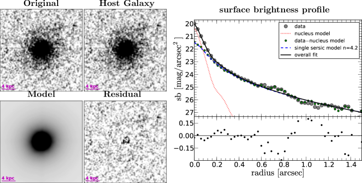
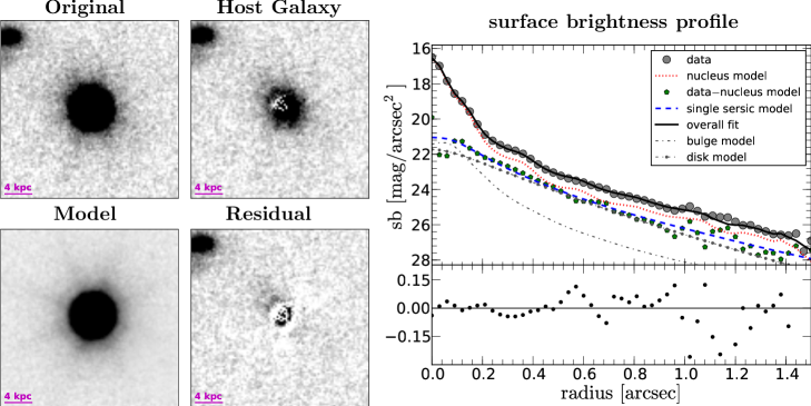
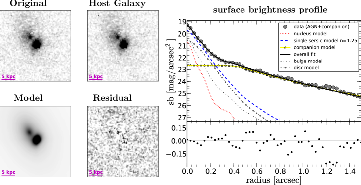
Figure 2.— Three examples of HST image decomposition and surface profile fitting. Top panels: AGN ID-158 having a bulge-to-total (B/T) light ratio equal to 1.0 based on the F606W filter band. The four images are as follows: (i) the original image (upper left), (ii) the host galaxy after removing the point source (upper right), (iii) the best fit model (lower left), and (iv) the residual after subtraction of the best fit model from the original image. The scaling is the same in all images. On the right (upper panel) we show the surface brightness profiles of the various components (i.e. the original data - filled gray circle, the nucleus model/PSF red dotted line, the host galaxy after removal of the PSF (green pentagon), the best fit single sersic model - dashed line and the overall fit as a solid line) In the lower panel we show the residual after subtraction of the best fit model profile from the data. The single Sersic fit indicates a early type galaxy; therefore, no further decomposition into bulge and disk components is necessary. Middle panel: AGN ID-417 (B/T=0.3) in the ACS/F850LP filter band. Bottom panel: AGN ID-333 (B/T=0.35) in ACS/F850LP filter band. Due to the large contribution of the companion to the surface brightness profile, we model the companion separately and show its component and contribution to the overall surface brightness profile. Both ID-417 and ID-333 have host galaxy emission that can be decomposed into bulge and disk components.

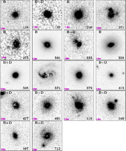
Figure 3.— Host galaxy images after removing the point source using GALFIT in the F850LP filter band for the whole sample. We have marked objects for which we could get a direct bulge estimate through either a pure bulge (B) or bulge+disk fit (B+D)

We use GALFIT (Peng et al., 2002, 2010) to fit the two-dimensional light distribution of each AGN with a point source model represented by an empirical PSF plus a Sersic model for the host galaxy. The nucleus component is either an average PSF created from various field stars around the target, or a single PSF star as described above. The decomposition of the images is done in several steps. First, we conservatively subtract a PSF scaled to the flux contained in a small aperture (typically 2 pixels) around the central pixel. For the second step, we perform a full decomposition by adding a Sersic model as a second component. We then optimize the fit to minimize the residuals. This step requires several iterations of the fit using different starting values to ensure convergence to a global minimum in the parameter space. If necessary, we add further components to fit asymmetries in the host (e.g., arm structures). Neighboring galaxies are either masked out or fitted simultaneously (see ID-333 for such an example in the bottom panel of Figure 2) to avoid flux spilling over from one object to the other. If the host galaxy flux is below 2%, we decide that the host galaxy is unresolved.

In Figure 2, we show three representative examples of the image decomposition procedure for objects with different nuclear-to-host (N/H) ratio and bulge-to-total (B/T) stellar light ratio. As shown, these cases demonstrate the effectiveness of both the short (F606W) and long (F850LP) wavelength HST imaging. The top panel shows ID-158 that exhibits a nuclear component attributed to the AGN and a clearly extended component characterized by a Sersic index of 4.2. With no discernable disk, the morphology is determined to be that of an early-type galaxy. In the middle panels, the host galaxy of AGN (ID-417) is well resolved above our detection limit even though it has a high N/H ratio. The Sersic index is found to be n=2.1 that does not favor either a simple early or late type morphology. Only through a decomposition of the bulge and disk components (as described below) can we determine whether this object is truly bulge or disk dominated. The third example (ID-333) shown in the bottom panels has a galaxy contribution with a Sersic index of 1.25 indicating a strong disk contribution to the overall morphology. In Table 1, we list the sample properties and the results of our fitting routine. In Figure 3, we show the PSF-subtracted host images of the entire sample.

We estimate the uncertainties of our measurements through a series of simulations. We create artificial AGN images using empirical PSFs and host galaxy models superimposed with artificial noise to match the flux levels measured in the real images. We estimate statistical errors on the host galaxy and nuclear magnitude by comparing the input and output values for our fit parameters. Host galaxy apparent magnitude, radius and morphology are extracted from the Sersic model fits. Since the Sersic index can be underestimated, in some cases, using GALFIT, especially when the nuclear-to-host (N/H) ratio is high (see Sánchez et al., 2004; Kim et al., 2008a, b), we use the simulations to correct the Sersic index. Here, we also want to point out the importance of the HST data again specially in cases such as ID-333 (See Fig. 2) where the AGN is strongly contaminated by a nearby companion that is hardly resolved in ground-based data.

A direct bulge/disk decomposition is only possible for objects which have low N/H ratios (typically $N/H<2$). We find 5/18 host galaxies to have $n_{sersic,corrected}>3$; therefore, we classify them as truly bulge dominated. If the single Sersic fit of the host galaxy indicates the possible presence of a disk component with $n_{sersic,corrected}<3$ (13/18 objects), we refit the galaxy with two Sersic models each representing the disk and the bulge. We put limits on the Sersic Index ($0.5<n<1.5$ for the disk and $3<n<5$ for the bulge) of each component to achieve an effectively reduced chi square of the residuals as compared to using single values typical for a disk (n=1) and bulge (n=4) components. In the end, we are able to directly decompose 14/18 host galaxies in the F850LP filter into either a purely bulge or bulge+disk component. Some bulge+disk component fits failed due to the disturbed morphology of the host galaxy (i.e. ID-271 or ID-516) even though the AGN was weak ($N/H<1$). Since the F850LP filter provides the best contrast between nuclear and host component, we can use the best fit parameters (i.e. disk/bulge radius, position angle, axis ratios) as constraint in the bluer filter bands with typically higher $N/H$ ratios. The best fit radii for the bulge components range from 0.6-6 kpc and are consistent with the typical sizes of elliptical galaxies at similar redshifts (Trujillo et al., 2007). In four cases, the radius of the bulge component is less than 3.5 pixel and the fit can be treated as an upper limit. But we also want to caution that the radii are more sensitive as a free parameter of the fit than the fluxes of the components.

We can further check whether the inclusion of a pseudo-bulge component provides a reasonable fit to the surface brightness profile. To do so, we allow the bulge component to have a lower Sersic index. While it is challenging to distinguish between a pseudo-bulge and a classical bulge with the data in hand, we do find stronger residuals in the nuclear region if we fit with a pseudo-bulge component. These new fits lead to only small changes in the fluxes of each component (¡0.1 mag) and bulge-to-disk ratio (¡13%), hence only a small impact on the stellar mass estimates. The poorer fits, seen when incorporating a pseudo-bulge component, may indicate that SMBHs are more directly related to classical bulges than pseudo-bulges (Kormendy et al., 2011).

For N/H$>$3, we estimate a bulge correction through extensive simulations rather than a direct measurement. For each filter band starting with the longest wavelength due to lower contrast between AGN and host galaxy, we create a set of artificial AGN+host images using the best fit parameters for the nucleus component. The host galaxy consists of two Sersic models, one for the disk and one for the bulge component. We vary the free parameters to mimic a broad range of bulges and disks. We add appropriate noise measured from the HST images and fit the artificial images with a single Sersic model plus PSF model. We compare the fit solutions of the simulations with our single Sersic fit of the real data and select the B/T ratios of all model fits that recover the original fit parameters within their uncertainties. We fit all filter bands separately to account for possible color gradients between the disk and the bulge. Due to higher N/H ratios at shorter wavelength and typically lower S/N (fainter objects) we constrain some of the free parameters such as size, ellipticity and centroid position to the range of solutions found in the F850LP filter band. In Figure 4, we show the B/T distributions recovered for two of our host galaxies (ID-417 and ID-375) together with an image of the host galaxy. Figure 4 also shows the good agreement between the recovered B/T ratio and the host morphology. For example ID-375 has a low B/T ratio of about 0.1 indicating the presence of a dominating disk and the image of the host galaxy shows some spiral structures with very little light concentration in the center of the galaxy. The mean value of the B/T distribution and its uncertainty is then used to estimate the bulge mass. The error bars on the photometry are typically larger by 0.15-0.3 mag.

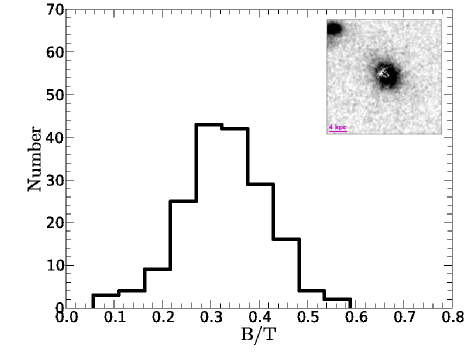
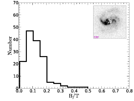
Figure 4.— B/T distribution of ID-417 (top) and ID-375 (bottom) extracted from our simulations matching the properties of the host galaxy using a single Sersic component. The insets shows the host galaxy in F850LP after removal of the nuclear point source.

3.2. Total/Bulge Stellar Mass Estimates

Our main goal is the estimation of the stellar mass content of each host galaxy and its bulge component in the sample by converting the rest frame optical colors into mass-to-light ratios. For targets in the GEMS area, we have only a single optical color while for GOODS we have multiple colors based on four filter bands. This method has been successfully employed in several studies on AGN host galaxies (e.g., Schramm et al., 2008; Jahnke et al., 2004, 2009; Sánchez et al., 2004). As demonstrated by Bell et al. (2003) for a variety of star formation histories, the stellar mass-to-light ratio (M/L) can be robustly predicted from the B-V color. We adopt their formula based on a Chabrier IMF:

$$\mathrm{log}_{10}(M/L_{V})=-0.728+(1.305\times(B-V))\>,$$ (1)

where $M/L_{V}$ is given in solar units. The choice of an IMF has a systematic effect on the final mass estimation. Using a Salpeter IMF would typically increase our mass-to-light ratios by factor of 1.4.

The ECDFS area is well covered by broad-band photometry from various instruments ranging from the ultraviolet to the infrared. The available photometry provides another approach to estimate the total stellar mass content of the host galaxies through direct SED fitting (as shown by Merloni et al. 2010). Although this would be a powerful alternative, the data suffers from additional uncertainties such as source confusion in the ground based data or variability of the sources due to multi-epoch data. In any case, we decided to implement SED fitting only as a consistency check on our total stellar mass estimates based on the HST data. For the procedure, we use our own algorithm based on a Levenberg-Marquart $\chi^{2}$ minimization. We use a set of SED model templates (Maraston, 2005) with declining star formation histories based on a Kroupa IMF (which gives similar results as a Chabrier IMF), solar metallicity and a dust extinction law following Calzetti et al. (2000). We make use of the broad-band image decomposition (AGN+host) based on the HST results to constrain the template models that includes the photometric errors in each filter band. First, we fit a template AGN model (Richards et al. 2006) to the photometry of the nucleus obtained from the decomposition and subtract this from the total (ground-and/or space-based) photometry. Next, we fit the residual fluxes with either a single template or a two component template. Strong contamination from unresolved sources in the ground based data (i.e. in ID-333) are taken into account and subtracted separately using the HST photometry as an additional constraint for the companion template model. To estimate errors on the stellar mass, we use a Monte Carlo approach. We vary the observed flux in each bandpass by a random number which is Gaussian distributed with a sigma defined by the flux error. We generate 100 simulated SEDs and recompute the fit. Masses from both approaches typically agree within 0.13 dex. In Figure 6, we show four examples (ID-339, ID-170, ID-465 and ID-250) of the SED decomposition compared to the single epoch spectrum used for the BH mass estimation. These four AGN represent different level of AGN and host stellar continuum throughout our sample. In addition, these objects also have different B/T ratios: 1.0 (ID-339, ID-250), 0.5 (ID-170) and 0.24 (ID-465). These examples illustrate the clear advantage gained from having the HST photometry. Only with HST resolution, we can constrain the flux of the AGN and the host galaxy including the bulge and disk components separately. The mass estimates from Bell et al. (2003) and SED fitting typically agree within 0.15 dex.

In Figure 6, we plot the U-V rest-frame color versus the total stellar mass. Nearly all hosts concentrate at the high mass end and below the red sequence (i.e., the green valley). The masses of our host galaxies are comparable to typical red sequence galaxies but the colors of the host indicate a population of recently formed stars.

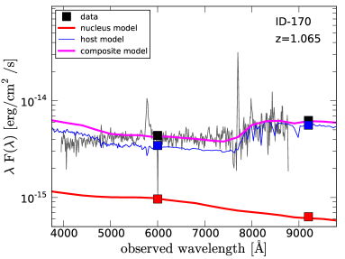
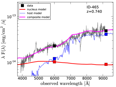
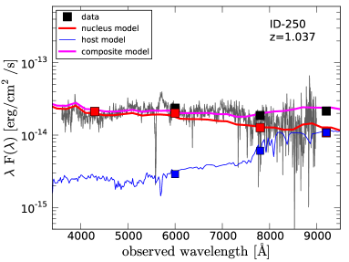
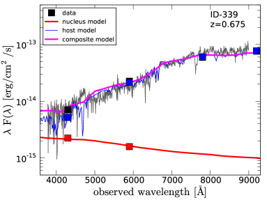
Figure 5.— Examples of the SED template fitting for different nuclear-to-host ratios (ID-339,ID-250; ID-170; ID-465). Black squares show the total photometry measured in the bands covered by HST (either F606W and F850LP for GEMS or F435W, F606W, F775W, F850LP for GOODS). Red and blue squares show the results from the image decomposition in the HST filter bands representing the nuclear component (red) and the host component (blue). The red and blue solid lines represent the best fit AGN and host galaxy models with the magenta solid line showing their sum.

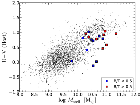
Figure 6.— Rest frame U-V color vs. total stellar mass of the host galaxy compared to a sample of inactive galaxies in the same redshift range taken from the GEMS catalog.

4. Black Hole Masses

We measure black hole masses for our entire type 1 AGN sample using single-epoch spectra that provide both a velocity width of a broad emission line and the monochromatic luminosity of the continuum. We use optical spectra acquired mainly from the followup of X-ray sources (Szokoly et al., 2004; Silverman et al., 2010). We supplement these with spectra taken with FORS2 on the VLT but not yet publicly available.

Several prescriptions to estimate black hole masses are available from the literature using various emission lines such as H$\beta$, MgII or CIV (Kaspi et al., 2000; Vestergaard & Peterson, 2006; Collin et al., 2006; McLure & Jarvis, 2002). Due to the redshift range of our sample and optical spectroscopic coverage, we use the MgII emission line to estimate virial black hole masses in all cases. Although most of the black hole mass calibrations are based on reverberation mapping data of $H\beta$ several studies have shown that there is good agreement between the mass estimates based on MgII and the Balmer lines ($H\beta$, H$\alpha$) out to high redshifts (Shen & Liu 2012; Matsuoka et al. 2012) by combining optical and NIR spectroscopy. The prescription for estimating black hole mass as given in McLure & Jarvis (2002) is implemented; although, we recognize that similar recipes are available elsewhere (Kong et al. 2006, McGill et al. 2008, Wang et al. 2009) with each of these agreeing essentially to within 0.2-0.3 dex.

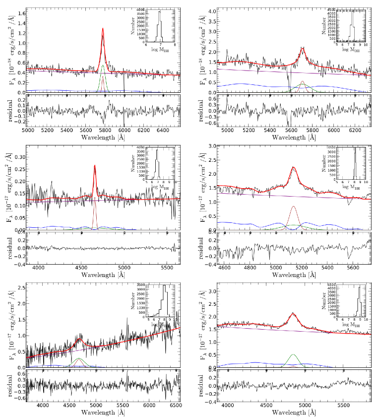
Figure 7.— Multicomponent fit to broad MgII emission line for six representative objects from our sample. The top panel shows the spectral range around the emission line. The best fit model is indicated as a red solid line. The different components are as indicated: Fe-emission (blue), pseudo-continuum (purple), Gaussian components (green and brown). The residual (data-fit) is shown in the lower panel. In the upper right corner of each panel, we show the black hole mass distribution computed from our Monte Carlo tests based on the uncertainties of the line width and continuum luminosity measurements. The objects are (from top left to bottom right): ID-170,ID-250,ID-413,ID-417,ID-339, and ID-379

We perform an iterative least-squares minimization to fit the MgII line for each AGN to measure its line width. Our procedure is a modified version of the one used in Gavignaud et al. (2008). The number of components to fit the line depends on the characteristics of the objects and quality of the data. We fit the region around the emission line using a model that includes a pseudo-continuum and one or two Gaussian components to characterize the line profile. We find that for the local continuum a powerlaw+broadened Fe-template (provided by M. Vestergaard: see Vestergaard & Wilkes, 2001) gives the best results. Specially the strength of the Fe-emission in the wings of the MgII line can vary strongly (see ID-250 for strong Fe and ID-170 for very weak Fe) and affects the outcome of the fit. We try to both minimize the number of model components and optimize the residuals around the emission line. We either interpolate over absorption features or mask them out. A FWHM of the line profile is determined using either a one or two component Gaussian model. We have tested the same algorithm on the sample from Merloni et al. (2010). Even tough we find some scatter for the individual fits, there is no systematic offset in the final black hole mass estimates. Two of our objects overlap with the study from Bennert et al. (2011b); our mass estimates agree within  0.1 dex using the same recipe.

In the next step, we measure the continuum luminosity at 3000 Å  required to estimate a radius to the BLR. For luminous AGN ($L_{\mathrm{bol}}>45$) the continuum luminosity can be directly measured from the spectrum due to the typically low impact of the host galaxy. For our sample, we find that in several cases, there is a significant host galaxy contribution that must be taken into account (see Fig. 5). Therefore, we decided to measure the monochromatic luminosity at 3000 Å  by decomposing the HST/ACS images. The procedure enables us to isolate the AGN (i.e., nuclear) emission from its host galaxy most effectively. We then fit an average quasar SED template (Richards et al., 2006), accounting for dust attenuation to estimate the intrinsic continuum luminosity at 3000 Å. We find that the continuum luminosity based on HST imaging agrees with that determined from the decomposition of the broad-band SED to within 5%. Monte Carlo realizations using the uncertainties of the FWHM and $L_{3000}$ measurements enable us to estimate the uncertainties on the black hole mass in addition to 0.4 dex uncertainty inherent in the scaling relations. In Figure 7, we present examples of the fits to the broad emission lines in six AGN with different quality of data. A summary of the results of our line fits are shown in Table 1.

5. Results

5.1. The BH Mass-Total Stellar Mass Relation

We first present the relation between black hole mass ($M_{\mathrm{BH}}$) and total stellar mass ($M_{\mathrm{*,Total}}$) in Figure 8 ($left$ panel). From the distribution of data points, it is apparent that our sample does not have the dynamic range in either stellar mass or black hole mass to establish both a slope and normalization simultaneously of a linear fit. Fortunately, we can compare with the local relation established using inactive galaxies (mainly ellipticals or S0) as done by Häring & Rix (2004) and determine whether an offset exists. We find that essentially all of our AGN fall along the local $M_{\mathrm{BH}}-M_{*,\mathrm{Bulge}}\,$relation. It is important to highlight that the bulge mass is equivalent to the total stellar mass for the local comparison sample. To be more specific, we find that 17/18 objects, considering their 1$\sigma$ errors, are consistent with the typical region of 0.3 dex scatter around the best fit local relation having a slope of 1.12 (Häring & Rix, 2004). Given our limitations in mass coverage as mentioned above, we fit a linear regression model to our data while fixing the slope to the value given above thus determining only the normalization. We find the best-fit normalization to be 8.31 by using FITEXY (Press et al., 1993), which estimates the parameters of a linear fit while considering errors on both variables. The fit is affected by the single target offset from the relation. If excluded for no obvious reason, the constant would be 8.24. With a simple Monte Carlo test, we can reject the null hypothesis that the two samples are significantly different. While the local inactive sample is established using dynamical masses, we do not expect these to differ substantially from the stellar masses; this is in fact the case as demonstrated in Bennert et al. (2011a).

Ideally, we would like to compare our sample with a local sample of active SMBHs with stellar mass measurements of their hosts. The work of Bennert et al. (2011a) allows such a direct comparison. We show these data in Figure 8 as marked by small black circles. Carrying out the same fit as for the ECDFS AGNs, we find the best fit constant to be 8.30 for the local AGNs. We use the total stellar mass for the regression fit of both active samples (Bennert et al. (2011a), ECDFS AGNs) and find no significant deviation between them in the $M_{\mathrm{BH}}-M_{*,\mathrm{Total}}\,$relation.

Our result agrees well with findings of recent studies of the $M_{\mathrm{BH}}-M_{\mathrm{*,Total}}$ relation at high redshift. In particular, Jahnke et al. (2009) use a similar technique of decomposing HST images and converting rest-frame optical colors into stellar mass-to-light ratios based on a sample of AGNs at $z>1$ in COSMOS with NICMOS coverage. Their sample consists of ten objects with seven for which they achieve a decomposition in multiple bands and find no offset in black hole mass given their total stellar masses. Our study effectively improves the statistics by a factor of 2.5 and fills in a gap in redshift coverage (see Figure 8, $right$ panel). In addition, these results are supported by the findings of Cisternas et al. (2011) who explored the same relation on a sample of BLAGN at $0.3<z<0.9$ from the COSMOS survey; although, only one HST band is available to constrain the stellar mass content of the host galaxy.

Taken together, these studies (Jahnke et al., 2009; Cisternas et al., 2011), including our own, clearly contrast with other works at high redshift that claim an increasing offset in black hole mass for a given stellar mass. In the right panel of Figure 8, we show the redshift evolution of $M_{\mathrm{BH}}$-$M_{\mathrm{*,Total}}$ ratio compared to various other studies probing the same relation. Some studies are using different mass estimators for the black hole masses or stellar masses. For example, Merloni et al. (2010) use the prescription of McGill et al. (2008) for their black hole mass estimations and assume a Salpeter IMF for their stellar mass estimates. When necessary, we convert the masses of different studies to the prescription based on the formula from McLure & Jarvis (2004) and a Chabrier IMF for the stellar mass estimates. In case of Merloni et al. (2010), the corrections have only a marginal effect on the $M_{\mathrm{BH}}-M_{\mathrm{*,Total}}$ relation. Based on our results, we cannot confirm or rule out a stronger evolution at higher redshift ($z>1.5$). In particular, our mean bolometric luminosity is log $L_{bol}=44.7$ while the higher redshift sample of Merloni et al. (2010) is at $log~{}L_{bol}=45.5$. As a consequence, the mean BH mass is shifted to higher masses and therefore a direct comparison with these objects and any trend implied by the data might be biased by the differences in the sample properties. It is worth highlighting that our results are likely to be less biased due to selection since our BH masses are typically below $10^{9}M_{\odot}$, the knee in the black hole mass function; we may be effectively avoiding the problems fully presented in Lauer et al. (2007).

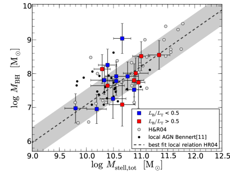
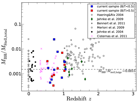
Figure 8.— Left: $M_{\mathrm{BH}}-M_{*,\mathrm{Total}}\,$relation for our sample of intermediate redshift AGN. The sample has been divided into bulge (red squares) and disk dominated (blue squares) systems based on our bulge corrections. The data is superimposed on the sample of inactive galaxies from Häring & Rix (2004) (dynamical mass) and the local AGN (stellar mass) sample from Bennert et al. (2011a). The dashed line represents the best fit from Häring & Rix 2004 with a 0.3 dex scatter shown as the grey shaded area. Right: Redshift evolution of the relation in comparision with several other studies taken from the literature. The dashed line shows the mean constant ratio from the local relation by Häring & Rix (2004).

5.2. The BH Mass-Bulge Stellar Mass Relation

While the total stellar mass is well-determined using different methods (Schramm et al., 2008; Jahnke et al., 2009; Merloni et al., 2010; Cisternas et al., 2011; Bennert et al., 2011b), we usually do not know how much of the total mass is present in the bulge. As stated above, only 5/18 of our AGN hosts have a Sersic Index $n>3$ indicating a purely bulge-dominated host galaxy. We make the assumption that for these objects the total mass is the same as the bulge mass. For the remainder, we estimate the bulge contribution to the total mass by corrections to the total mass by accounting for the contribution of the disk. Applying the same cut at $n<3$, we find that $\sim$72% of the host galaxies show a disk component. Although the fraction is in good agreement with the results presented by Schawinski et al. (2011) on a sample of X-ray selected AGN in the $Chandra$ Deep Field South at $2<z<3$. Although, we draw a different conclusion on the importance of the disk component, in terms of the mass contribution to the total mass. Our bulge/disk decomposition shows that, even though a disk is present, the mass of the central bulge can still dominate the total mass of the host galaxy. The different redshift regimes might play an important role since there is about 3-5 Gyr of galaxy evolution between our study and that of Schawinski et al. (2011). Using the B/T ratio to divide our sample into bulge and disk dominated systems, we find that $\sim 50$% of the sample has a significant bulge component with $B/T>0.5$; this can even be true for objects with a surface brightness profile of the host galaxy described by a fit with a Sersic index of $\sim$2.

We can now establish the $M_{\mathrm{BH}}-M_{*,\mathrm{Bulge}}\,$relation at $0.5<z<1.2$. In Figure 9, we plot the $M_{\mathrm{BH}}-M_{*,\mathrm{Bulge}}\,$relation and compare our results with the sample of inactive galaxies from Häring & Rix (2004) and local AGN from Bennert et al. (2011a). The stellar mass measurements for the local AGN allow a more direct comparison with our sample than the dynamical masses of Häring & Rix (2004). We find that the mass distributions for all three samples are very similar with each other. This can be clearly seen in a histogram of the mass ratio ($log~{}M_{BH}/M_{*,Bulge}$) shown in the top panel of Figure 10, where there is no significant difference in the median value. Overall, we find that 78% of the AGNs are consistent with the local relation. If we consider the single object undergoing a clear major merger (ID-333), there are only three objects that are significantly offset from the local relation. If we artificially move this object onto the relation, then 83% of AGNs in our sample are consistent with the local relation. We interpret this as evidence for a black hole-bulge relation, at these redshifts, to be similar to the local relation. Interestingly, we do find additional scatter in our sample compared to that in the local distributions. We further note that there are no objects well below the $M_{\mathrm{BH}}-M_{*,\mathrm{Bulge}}\,$relation.

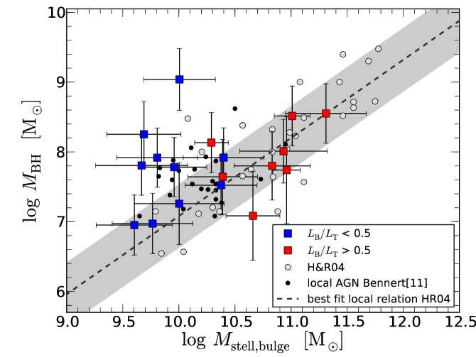
Figure 9.— $M_{\mathrm{BH}}-M_{*,\mathrm{Bulge}}\,$relation for our sample of intermediate redshift AGN. Symbols are the same as in Figure 8

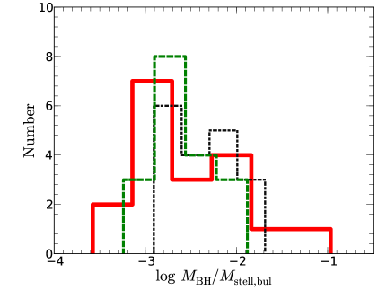
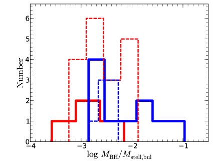
Figure 10.— $Top$ panel: $M_{\mathrm{BH}}-M_{*,\mathrm{Bulge}}\,$ratio distribution for our sample of intermediate redshift AGN (red solid) compared to the sample of inactive (black dotted) and active (green dashed) galaxies from Bennert et al. (2011a) using stellar host galaxy masses. The inactive sample from Bennert et al. (2011b) is based on the group 1 sample from Marconi & Hunt (2003) which overlaps also with the sample of Häring & Rix 2004. $Bottom$ panel: Comparision of the $M_{\mathrm{BH}}-M_{*,\mathrm{Bulge}}\,$ratio distribution for the bulge dominated ($L_{B}/L_{T}>0.5$) subsample shown as red solid line, the disk dominated ($L_{B}/L_{T}<0.5$) subsample shown as blue solid line. The data is superimposed on the sample of local AGN from Bennert et al. (2011a) showing the sample separation into bulge (red dashed) and disk (blue dashed) dominated systems.

We can further investigate where high-z AGN lie in respect to the local relation as a function of their bulge-to-total ratio. All objects with $B/T>0.5$ fall nicely onto the local relation (see Figure 9 and the bottom panel of  10). They are also the most massive objects in the sample in terms of their bulge mass. Objects with a $B/T<0.5$ are clearly separated in bulge mass (from bulge-dominated objects) and the majority are still in good agreement with the local relation. Only four objects have under massive bulges considering their $1\sigma$ error bars including ID-333 which has a massive companion that might move the whole system onto the relation after the merger.

6. Discussion

An important question for SMBHs and their host galaxies is their subsequent evolution in the black hole - bulge mass plane. As previously mentioned, 83% of the bulges in our sample are already massive enough that their $M_{\mathrm{BH}}-M_{*,\mathrm{Bulge}}\,$ratio agrees well with that seen in inactive galaxies today (see Figure 9). We illustrate this further in Figure 10 (top panel), by comparing the distribution of the $M_{\mathrm{BH}}-M_{*,\mathrm{Bulge}}\,$ratio between various samples. Interestingly, there are some outliers with undermassive bulges, relative to their BH mass, that are preferentially disk dominated galaxies. In the bottom panel of Figure 10, we compare the distributions of this ratio for the bulge and disk dominated subsamples separately to the distribution of the local AGNs. Even though the number statistics are small, we find no difference for the bulge dominated subsample by looking at their median ratios. The situation is different for objects in the disk-dominated subsample. While some objects overlap with the distribution $M_{\mathrm{BH}}-M_{*,\mathrm{Bulge}}\,$ratios of the local AGN, the median ratio of the disk dominated subsample is shifted by 0.5 dex towards a higher ratio. When comparing bulges of similar mass ($\mathrm{log}\,M_{\mathrm{*,Bulge}}<10.5$), local AGN host galaxies have a smaller offset ($\sim$0.25 dex). On the other hand for the same mass matched subsample which includes 22/25 objects in the local AGN sample and 12/18 from our sample, we find that the local AGN sample contains only $\sim$30% disk dominated systems while our subsample contains $\sim 80\%$ disk dominated systems. Within the AGN population, we may be witnessing both a migration onto the local relation and a morphological transformation with cosmic time. We recognize that selection effects may impact such comparisons. Ideally, we want to have an AGN sample spanning a wide baseline in redshift with equivalent selection, BH mass indicators and sufficient statistics.

This leads to the question how these host galaxies can grow their stellar bulge mass to match the bulge masses seen today. One possible track could be the event of a major merger that leads ultimately to a significant increase in stellar bulge mass. Mergers are seen to play a role in black hole growth for similar X-ray selected samples (Silverman et al., 2011). Out of our 18 AGN, only one (ID-333) shows signs of an ongoing major merger. Even though other host galaxies do show some signs of minor merger activity, we conclude that the growth of the bulge through a major merger event in the near future is not certain. On the other hand, the good agreement of the AGN host galaxy $M_{\mathrm{BH}}$-$M_{\mathrm{*,Total}}$ relation with the local relation clearly shows that all the mass needed to put our host galaxies onto the local $M_{\mathrm{BH}}-M_{*,\mathrm{Bulge}}\,$relation is already in place within these galaxies at redshift $z\sim 1$ (Jahnke et al., 2009). Therefore, mass transfer from the disk to the bulge is neccessary to grow their bulges. Any bulge growth through internal processes has to overcome the mass growth of the black hole otherwise the galaxy would just move on a diagonal track in the $M_{\mathrm{BH}}-M_{*,\mathrm{Bulge}}\,$relation.

While the BHs in their active phase are growing, we can also investigate how the host galaxy is growing in stellar mass by looking at their individual growth rates (i.e., SFR) and compare these to the BH growth rates. We estimate star-formation rates based on the UV continuum from our best fit SED models and converted these into growth rates (SFR/$M_{\mathrm{stell}}$). In Figure 11, we compare the growth rates of the host galaxies with the growth rates of the BHs as determined by $\dot{M}/M_{\mathrm{BH}}$. $\dot{M}$ is determined from $L_{bol}=\epsilon\dot{M}c^{2}$. To estimate the bolometric luminosities $L_{bol}$ and Eddington ratios, we use the luminosity dependent corrections from Hopkins et al. (2007) applied to our derived continuum luminosities at 3000 Å. We find that apparently the BHs gain mass much stronger than the host galaxies by a factor of $\sim$30. These relative growth rates are broadly consistent with that seen in obscured AGN (Netzer, 2009; Silverman et al., 2009). Such an offset implies that the typical duty cycle of an AGN (see Martini (2004) for an overview) during which it can grow its BH mass efficiently must be short enough (typically $~{}10^{7}-10^{8}$ yr) to prevent a significant vertical movement in the black hole mass - bulge mass plane. If the growth rates are extrapolated over a period of 1Gyr, the host galaxies do not gain much stellar mass from the present level of star formation. As previously mentioned, only one object (ID-333) shows a possible major merger due to the presence of a more massive but inactive companion. While some objects show signs of minor merging activity (i.e. ID-712,ID-271), and we cannot exclude that we miss further minor merger events due to their low surface brightness, the stellar mass gain is expected to be low. Assuming the current growth rates and ignoring a possible major merger, all galaxies except one would need more than $>\sim 1$Gyr to move more than 0.3 dex in the $M_{\mathrm{BH}}$-$M_{\mathrm{*,Total}}$. Therefore, we do not expect much evolution over the next 1Gyr for the majority of our sample.

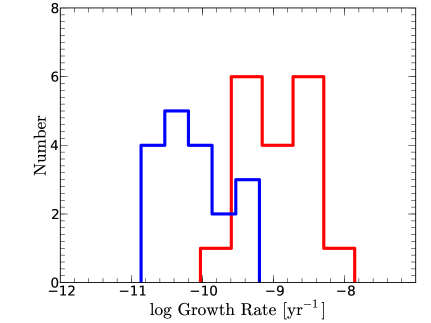
Figure 11.— Comparision of the growth rate distributions of the host galaxy (blue; $M_{*,Total}/SFR$) estimated from the UV-SFR and the BHs (red; $M_{BH}\times(dM/dt)^{-1}$) of our sample

7. Summary

We have performed a detailed analysis of a sample of 18 type 1 AGN host galaxies at $0.5<z<1.2$ to estimate their stellar mass content and explore the relation between the mass of the central BH and the mass of the host galaxy. Our sample is of moderate-luminosity due to a selection based initially on their X-ray emission as detected with the Extended $Chandra$ Deep Field - South Survey. This results in a sample having black hole masses below the knee of the black hole mass function thus mitigating biases (Lauer et al., 2007) seen in other samples to date. For the chosen redshift range, HST imaging is available with at least two filters that bracket the 4000 Å  break thus providing reliable stellar mass estimates of the host galaxy by accounting for both young and old stellar populations. We have estimated bulge masses for all galaxies through either direct decomposition of the imaging data into a bulge or bulge plus disk component, or through simulations where artificial host galaxies with different B/T ratios are compared to single Sersic fits of the host galaxy. We are now able to look separately into their relation of the BH mass with either total stellar mass content or bulge mass after the contribution from the disk is removed.

We find that the relation between $M_{\mathrm{BH}}$ and $M_{\mathrm{*,Total}}$ is in very good agreement with the local $M_{\mathrm{BH}}-M_{*,\mathrm{Bulge}}\,$which has been reported by several studies so far. From our morphological analysis and decomposition of bulge and disk components, we can quantify the fraction of bulge dominated objects with $B/T>0.5$ to be 50% while 72% of the sample shows the presence of a disk component which is a significantly higher fraction than for a stellar mass matched local AGN sample. Even though the bulge mass is shifted towards lower masses given their BH mass in some cases, we find that $\sim$80% of the sample is in agreement with the local $M_{\mathrm{BH}}$ and $M_{\mathrm{*,Bulge}}$ relation given their $1\sigma$ error bars. We further compare the growth rates of the host galaxy and their BHs and find that assuming the present SFR and accretion rates (while ignoring possible major merger events), only one AGN in our sample would move more than 0.3 dex over the next 1Gyr. We highlight that bulge dominated galaxies are well in place at $z\sim 1$ on the local $M_{\mathrm{BH}}-M_{*,\mathrm{Bulge}}\,$relation. There is a significant fraction (20%) of our sample that is disk dominated and above the local relation which is not seen in either local inactive or active galaxy samples. For these galaxies to grow their bulges and align themselves on the local relation a physical mechanism is likely needed to redistribute their stars. While mergers may play a role, it is not yet clear whether this is the dominant process.

References

- Ammons et al. (2009) Ammons, S. M., Melbourne, J., Max, C. E., Koo, D. C., & Rosario, D. J. V. 2009, AJ, 137, 470
- Bell et al. (2003) Bell, E. F., McIntosh, D. H., Katz, N., & Weinberg, M. D. 2003, ApJS, 149, 289
- Bennert et al. (2011a) Bennert, V. N., Auger, M. W., Treu, T., Woo, J.-H., & Malkan, M. A. 2011a, ApJ, 726, 59
- Bennert et al. (2011b) —. 2011b, ApJ, 742, 107
- Brusa et al. (2009) Brusa, M., Fiore, F., Santini, P., Grazian, A., Comastri, A., Zamorani, G., Hasinger, G., Merloni, A., Civano, F., Fontana, A., & Mainieri, V. 2009, A&A, 507, 1277
- Calzetti et al. (2000) Calzetti, D., Armus, L., Bohlin, R. C., Kinney, A. L., Koornneef, J., & Storchi-Bergmann, T. 2000, ApJ, 533, 682
- Cardamone et al. (2010) Cardamone, C. N., van Dokkum, P. G., Urry, C. M., Taniguchi, Y., Gawiser, E., Brammer, G., Taylor, E., Damen, M., Treister, E., Cobb, B. E., Bond, N., Schawinski, K., Lira, P., Murayama, T., Saito, T., & Sumikawa, K. 2010, ApJS, 189, 270
- Cisternas et al. (2011) Cisternas, M., Jahnke, K., Inskip, K. J., Kartaltepe, J., Koekemoer, A. M., Lisker, T., Robaina, A. R., Scodeggio, M., Sheth, K., Trump, J. R., Andrae, R., Miyaji, T., Lusso, E., Brusa, M., Capak, P., Cappelluti, N., Civano, F., Ilbert, O., Impey, C. D., Leauthaud, A., Lilly, S. J., Salvato, M., Scoville, N. Z., & Taniguchi, Y. 2011, ApJ, 726, 57
- Collin et al. (2006) Collin, S., Kawaguchi, T., Peterson, B. M., & Vestergaard, M. 2006, A&A, 456, 75
- Decarli et al. (2010a) Decarli, R., Falomo, R., Treves, A., Kotilainen, J. K., Labita, M., & Scarpa, R. 2010a, MNRAS, 402, 2441
- Decarli et al. (2010b) Decarli, R., Falomo, R., Treves, A., Labita, M., Kotilainen, J. K., & Scarpa, R. 2010b, MNRAS, 402, 2453
- Gavignaud et al. (2008) Gavignaud, I., Wisotzki, L., Bongiorno, A., Paltani, S., Zamorani, G., Møller, P., Le Brun, V., Husemann, B., Lamareille, F., Schramm, M., Le Fèvre, O., Bottini, D., Garilli, B., Maccagni, D., Scaramella, R., Scodeggio, M., Tresse, L., Vettolani, G., Zanichelli, A., Adami, C., Arnaboldi, M., Arnouts, S., Bardelli, S., Bolzonella, M., Cappi, A., Charlot, S., Ciliegi, P., Contini, T., Foucaud, S., Franzetti, P., Guzzo, L., Ilbert, O., Iovino, A., McCracken, H. J., Marano, B., Marinoni, C., Mazure, A., Meneux, B., Merighi, R., Pellò, R., Pollo, A., Pozzetti, L., Radovich, M., Zucca, E., Bondi, M., Busarello, G., Cucciati, O., de La Torre, S., Gregorini, L., Mellier, Y., Merluzzi, P., Ripepi, V., Rizzo, D., & Vergani, D. 2008, A&A, 492, 637
- Gebhardt et al. (2000) Gebhardt, K., Bender, R., Bower, G., Dressler, A., Faber, S. M., Filippenko, A. V., Green, R., Grillmair, C., Ho, L. C., Kormendy, J., Lauer, T. R., Magorrian, J., Pinkney, J., Richstone, D., & Tremaine, S. 2000, ApJL, 539, L13
- Giavalisco et al. (2004) Giavalisco, M., Ferguson, H. C., Koekemoer, A. M., Dickinson, M., Alexander, D. M., Bauer, F. E., Bergeron, J., Biagetti, C., Brandt, W. N., Casertano, S., Cesarsky, C., Chatzichristou, E., Conselice, C., Cristiani, S., Da Costa, L., Dahlen, T., de Mello, D., Eisenhardt, P., Erben, T., Fall, S. M., Fassnacht, C., Fosbury, R., Fruchter, A., Gardner, J. P., Grogin, N., Hook, R. N., Hornschemeier, A. E., Idzi, R., Jogee, S., Kretchmer, C., Laidler, V., Lee, K. S., Livio, M., Lucas, R., Madau, P., Mobasher, B., Moustakas, L. A., Nonino, M., Padovani, P., Papovich, C., Park, Y., Ravindranath, S., Renzini, A., Richardson, M., Riess, A., Rosati, P., Schirmer, M., Schreier, E., Somerville, R. S., Spinrad, H., Stern, D., Stiavelli, M., Strolger, L., Urry, C. M., Vandame, B., Williams, R., & Wolf, C. 2004, ApJ, 600, L93
- Grogin et al. (2005) Grogin, N. A., Conselice, C. J., Chatzichristou, E., Alexander, D. M., Bauer, F. E., Hornschemeier, A. E., Jogee, S., Koekemoer, A. M., Laidler, V. G., Livio, M., Lucas, R. A., Paolillo, M., Ravindranath, S., Schreier, E. J., Simmons, B. D., & Urry, C. M. 2005, ApJ, 627, L97
- Häring & Rix (2004) Häring, N. & Rix, H.-W. 2004, ApJ, 604, L89
- Hopkins et al. (2007) Hopkins, P. F., Richards, G. T., & Hernquist, L. 2007, ApJ, 654, 731
- Jahnke et al. (2009) Jahnke, K., Bongiorno, A., Brusa, M., Capak, P., Cappelluti, N., Cisternas, M., Civano, F., Colbert, J., Comastri, A., Elvis, M., Hasinger, G., Impey, C., Inskip, K., Koekemoer, A. M., Lilly, S., Maier, C., Merloni, A., Riechers, D., Salvato, M., Schinnerer, E., Scoville, N. Z., Silverman, J., Taniguchi, Y., Trump, J. R., & Yan, L. 2009, ArXiv e-prints
- Jahnke et al. (2004) Jahnke, K., Kuhlbrodt, B., & Wisotzki, L. 2004, MNRAS, 352, 399
- Kaspi et al. (2000) Kaspi, S., Smith, P. S., Netzer, H., Maoz, D., Jannuzi, B. T., & Giveon, U. 2000, ApJ, 533, 631
- Kim et al. (2008a) Kim, M., Ho, L. C., Peng, C. Y., Barth, A. J., & Im, M. 2008a, ApJS, 179, 283
- Kim et al. (2008b) Kim, M., Ho, L. C., Peng, C. Y., Barth, A. J., Im, M., Martini, P., & Nelson, C. H. 2008b, ApJ, 687, 767
- Kormendy et al. (2011) Kormendy, J., Bender, R., & Cornell, M. E. 2011, Nature, 469, 374
- Kormendy & Richstone (1995) Kormendy, J. & Richstone, D. 1995, ARA&A, 33, 581
- Lauer et al. (2007) Lauer, T. R., Tremaine, S., Richstone, D., & Faber, S. M. 2007, ApJ, 670, 249
- Lehmer et al. (2005) Lehmer, B. D., Brandt, W. N., Alexander, D. M., Bauer, F. E., Schneider, D. P., Tozzi, P., Bergeron, J., Garmire, G. P., Giacconi, R., Gilli, R., Hasinger, G., Hornschemeier, A. E., Koekemoer, A. M., Mainieri, V., Miyaji, T., Nonino, M., Rosati, P., Silverman, J. D., Szokoly, G., & Vignali, C. 2005, ApJS, 161, 21
- Magorrian et al. (1998) Magorrian, J., Tremaine, S., Richstone, D., Bender, R., Bower, G., Dressler, A., Faber, S. M., Gebhardt, K., Green, R., Grillmair, C., Kormendy, J., & Lauer, T. 1998, AJ, 115, 2285
- Maraston (2005) Maraston, C. 2005, MNRAS, 362, 799
- Marconi & Hunt (2003) Marconi, A. & Hunt, L. K. 2003, ApJ, 589, L21
- Martini (2004) Martini, P. 2004, Coevolution of Black Holes and Galaxies, 169
- McGill et al. (2008) McGill, K. L., Woo, J.-H., Treu, T., & Malkan, M. A. 2008, ApJ, 673, 703
- McLure & Jarvis (2002) McLure, R. J. & Jarvis, M. J. 2002, MNRAS, 337, 109
- McLure & Jarvis (2004) —. 2004, MNRAS, 353, L45
- Merloni et al. (2010) Merloni, A., Bongiorno, A., Bolzonella, M., Brusa, M., Civano, F., Comastri, A., Elvis, M., Fiore, F., Gilli, R., Hao, H., Jahnke, K., Koekemoer, A. M., Lusso, E., Mainieri, V., Mignoli, M., Miyaji, T., Renzini, A., Salvato, M., Silverman, J., Trump, J., Vignali, C., Zamorani, G., Capak, P., Lilly, S. J., Sanders, D., Taniguchi, Y., Bardelli, S., Carollo, C. M., Caputi, K., Contini, T., Coppa, G., Cucciati, O., de la Torre, S., de Ravel, L., Franzetti, P., Garilli, B., Hasinger, G., Impey, C., Iovino, A., Iwasawa, K., Kampczyk, P., Kneib, J.-P., Knobel, C., Kovač, K., Lamareille, F., Le Borgne, J.-F., Le Brun, V., Le Fèvre, O., Maier, C., Pello, R., Peng, Y., Perez Montero, E., Ricciardelli, E., Scodeggio, M., Tanaka, M., Tasca, L. A. M., Tresse, L., Vergani, D., & Zucca, E. 2010, ApJ, 708, 137
- Merritt & Ferrarese (2001) Merritt, D. & Ferrarese, L. 2001, MNRAS, 320, L30
- Netzer (2009) Netzer, H. 2009, MNRAS, 399, 1907
- Peng et al. (2002) Peng, C. Y., Ho, L. C., Impey, C. D., & Rix, H.-W. 2002, AJ, 124, 266
- Peng et al. (2010) —. 2010, AJ, 139, 2097
- Peng et al. (2006a) Peng, C. Y., Impey, C. D., Ho, L. C., Barton, E. J., & Rix, H.-W. 2006a, ApJ, 640, 114
- Peng et al. (2006b) Peng, C. Y., Impey, C. D., Rix, H.-W., Falco, E. E., Keeton, C. R., Kochanek, C. S., Lehár, J., & McLeod, B. A. 2006b, New Astronomy Review, 50, 689
- Pierce et al. (2007) Pierce, C. M., Lotz, J. M., Laird, E. S., Lin, L., Nandra, K., Primack, J. R., Faber, S. M., Barmby, P., Park, S. Q., Willner, S. P., Gwyn, S., Koo, D. C., Coil, A. L., Cooper, M. C., Georgakakis, A., Koekemoer, A. M., Noeske, K. G., Weiner, B. J., & Willmer, C. N. A. 2007, ApJ, 660, L19
- Press et al. (1993) Press, W. H., Teukolsky, S. A., Vetterling, W. T., & Flannery, B. P. 1993, Numerical Recipes in C: The Art of Scientific Computing, 2nd edn. (Cambridge, UK: Cambridge University Press)
- Richards et al. (2006) Richards, G. T., Strauss, M. A., Fan, X., Hall, P. B., Jester, S., Schneider, D. P., Vanden Berk, D. E., Stoughton, C., Anderson, S. F., Brunner, R. J., Gray, J., Gunn, J. E., Ivezić, Ž., Kirkland, M. K., Knapp, G. R., Loveday, J., Meiksin, A., Pope, A., Szalay, A. S., Thakar, A. R., Yanny, B., York, D. G., Barentine, J. C., Brewington, H. J., Brinkmann, J., Fukugita, M., Harvanek, M., Kent, S. M., Kleinman, S. J., Krzesiński, J., Long, D. C., Lupton, R. H., Nash, T., Neilsen, Jr., E. H., Nitta, A., Schlegel, D. J., & Snedden, S. A. 2006, AJ, 131, 2766
- Rix et al. (2004) Rix, H.-W., Barden, M., Beckwith, S. V. W., Bell, E. F., Borch, A., Caldwell, J. A. R., Häussler, B., Jahnke, K., Jogee, S., McIntosh, D. H., Meisenheimer, K., Peng, C. Y., Sanchez, S. F., Somerville, R. S., Wisotzki, L., & Wolf, C. 2004, ApJS, 152, 163
- Salviander et al. (2007) Salviander, S., Shields, G. A., Gebhardt, K., & Bonning, E. W. 2007, ApJ, 662, 131
- Sánchez et al. (2004) Sánchez, S. F., Jahnke, K., Wisotzki, L., McIntosh, D. H., Bell, E. F., Barden, M., Beckwith, S. V. W., Borch, A., Caldwell, J. A. R., Häussler, B., Jogee, S., Meisenheimer, K., Peng, C. Y., Rix, H.-W., Somerville, R. S., & Wolf, C. 2004, ApJ, 614, 586
- Schawinski et al. (2011) Schawinski, K., Treister, E., Urry, C. M., Cardamone, C. N., Simmons, B., & Yi, S. K. 2011, ApJ, 727, L31
- Schramm et al. (2008) Schramm, M., Wisotzki, L., & Jahnke, K. 2008, A&A, 478, 311
- Silverman et al. (2011) Silverman, J. D., Kampczyk, P., Jahnke, K., Andrae, R., Lilly, S. J., Elvis, M., Civano, F., Mainieri, V., Vignali, C., Zamorani, G., Nair, P., Le Fèvre, O., de Ravel, L., Bardelli, S., Bongiorno, A., Bolzonella, M., Cappi, A., Caputi, K., Carollo, C. M., Contini, T., Coppa, G., Cucciati, O., de la Torre, S., Franzetti, P., Garilli, B., Halliday, C., Hasinger, G., Iovino, A., Knobel, C., Koekemoer, A. M., Kovač, K., Lamareille, F., Le Borgne, J.-F., Le Brun, V., Maier, C., Mignoli, M., Pello, R., Pérez-Montero, E., Ricciardelli, E., Peng, Y., Scodeggio, M., Tanaka, M., Tasca, L., Tresse, L., Vergani, D., Zucca, E., Brusa, M., Cappelluti, N., Comastri, A., Finoguenov, A., Fu, H., Gilli, R., Hao, H., Ho, L. C., & Salvato, M. 2011, ApJ, 743, 2
- Silverman et al. (2009) Silverman, J. D., Lamareille, F., Maier, C., Lilly, S. J., Mainieri, V., Brusa, M., Cappelluti, N., Hasinger, G., Zamorani, G., Scodeggio, M., Bolzonella, M., Contini, T., Carollo, C. M., Jahnke, K., Kneib, J.-P., Le Fèvre, O., Merloni, A., Bardelli, S., Bongiorno, A., Brunner, H., Caputi, K., Civano, F., Comastri, A., Coppa, G., Cucciati, O., de la Torre, S., de Ravel, L., Elvis, M., Finoguenov, A., Fiore, F., Franzetti, P., Garilli, B., Gilli, R., Iovino, A., Kampczyk, P., Knobel, C., Kovač, K., Le Borgne, J.-F., Le Brun, V., Mignoli, M., Pello, R., Peng, Y., Perez Montero, E., Ricciardelli, E., Tanaka, M., Tasca, L., Tresse, L., Vergani, D., Vignali, C., Zucca, E., Bottini, D., Cappi, A., Cassata, P., Fumana, M., Griffiths, R., Kartaltepe, J., Koekemoer, A., Marinoni, C., McCracken, H. J., Memeo, P., Meneux, B., Oesch, P., Porciani, C., & Salvato, M. 2009, ApJ, 696, 396
- Silverman et al. (2008) Silverman, J. D., Mainieri, V., Lehmer, B. D., Alexander, D. M., Bauer, F. E., Bergeron, J., Brandt, W. N., Gilli, R., Hasinger, G., Schneider, D. P., Tozzi, P., Vignali, C., Koekemoer, A. M., Miyaji, T., Popesso, P., Rosati, P., & Szokoly, G. 2008, ApJ, 675, 1025
- Silverman et al. (2010) Silverman, J. D., Mainieri, V., Salvato, M., Hasinger, G., Bergeron, J., Capak, P., Szokoly, G., Finoguenov, A., Gilli, R., Rosati, P., Tozzi, P., Vignali, C., Alexander, D. M., Brandt, W. N., Lehmer, B. D., Luo, B., Rafferty, D., Xue, Y. Q., Balestra, I., Bauer, F. E., Brusa, M., Comastri, A., Kartaltepe, J., Koekemoer, A. M., Miyaji, T., Schneider, D. P., Treister, E., Wisotski, L., & Schramm, M. 2010, ApJS, 191, 124
- Szokoly et al. (2004) Szokoly, G. P., Bergeron, J., Hasinger, G., Lehmann, I., Kewley, L., Mainieri, V., Nonino, M., Rosati, P., Giacconi, R., Gilli, R., Gilmozzi, R., Norman, C., Romaniello, M., Schreier, E., Tozzi, P., Wang, J. X., Zheng, W., & Zirm, A. 2004, ApJS, 155, 271
- Trujillo et al. (2007) Trujillo, I., Conselice, C. J., Bundy, K., Cooper, M. C., Eisenhardt, P., & Ellis, R. S. 2007, MNRAS, 382, 109
- Vestergaard & Peterson (2006) Vestergaard, M. & Peterson, B. M. 2006, ApJ, 641, 689
- Vestergaard & Wilkes (2001) Vestergaard, M. & Wilkes, B. J. 2001, ApJS, 134, 1
- Woo et al. (2008) Woo, J., Treu, T., Malkan, M. A., & Blandford, R. D. 2008, ApJ, 681, 925
- Xue et al. (2010) Xue, Y. Q., Brandt, W. N., Luo, B., Rafferty, D. A., Alexander, D. M., Bauer, F. E., Lehmer, B. D., Schneider, D. P., & Silverman, J. D. 2010, ApJ, 720, 368