Nonlinear Force-Free Magnetic Field Fitting to Coronal Loops with and without Stereoscopy

Abstract

We developed a new nonlinear force-free magnetic field (NLFFF) forward-fitting algorithm based on an analytical approximation of force-free and divergence-free NLFFF solutions, which requires as input a line-of-sight magnetogram and traced 2D loop coordinates of coronal loops only, in contrast to stereoscopically triangulated 3D loop coordinates used in previous studies. Test results of simulated magnetic configurations and from four active regions observed with STEREO demonstrate that NLFFF solutions can be fitted with equal accuracy with or without stereoscopy, which relinquishes the necessity of STEREO data for magnetic modeling of active regions (on the solar disk). The 2D loop tracing method achieves a 2D misalignment of $\mu_{2}=2.7^{\circ}\pm 1.3^{\circ}$ between the model field lines and observed loops, and an accuracy of $\approx 1.0\%$ for the magnetic energy or free magnetic energy ratio. The three times higher spatial resolution of TRACE or SDO/AIA (compared with STEREO) yields also a proportionally smaller misalignment angle between model fit and observations. Visual/manual loop tracings are found to produce more accurate magnetic model fits than automated tracing algorithms. The computation time of the new forward-fitting code amounts to a few minutes per active region.

1 INTRODUCTION

The success or failure of magnetic field modeling of the solar corona depends on both the choice of the theoretical model, as well as on the choice of the used data sets. The simplest method is potential field modeling, which requires only a line-of-sight magnetogram $B_{z}(x,y,z_{phot})$, but only few solar active regions match a potential field model. Also linear force-free field (LFFF) models are generally considered as unrealistic, where a single constant value for the force-free parameter $\alpha$ represents the multi-current system of an entire active region in the solar corona. The state-of-the-art is the nonlinear force-free field (NLFFF) model, which can accomodate for an arbitrary configuration of current systems, described by a spatially varying $\alpha({\bf x})$ parameter distribution in an active region. The next strategic decision is the choice of data sets to constrain the theoretical model. NLFFF models generally require vector magnetograph data, ${\bf B}(x,y,z_{phot})=[B_{x}(x,y,z_{phot}),B_{y}(x,y,z_{phot}),B_{z}(x,y,z_{phot})]$, which are used as a lower boundary constraint and are extrapolated into the corona. However, a fundamental problem that has been identified is that the zone in the photosphere and lower chromosphere is not force-free (Metcalf et al., 1995), which spoils the extrapolation into coronal heights and leads to a substantial mismatch between the extrapolated field lines and observed coronal loops, typically amounting to a 3D misalignment angle of $\mu\approx 24^{\circ}-44^{\circ}$ (DeRosa et al., 2009; Sandman et al., 2009). Obviously, this fundamental problem can only be circumvented by using additional constraints from coronal data, since the corona above the transition region is generally force-free, except when the plasma-$\beta$ parameter is larger than unity (e.g., in filaments) or when the equilibrium brakes down (e.g., during filament eruptions, flares, and coronal mass ejections).

The problem amounts now how to implement coronal data into a theoretical magnetic field model, such as coronal loops, which are believed to be reliable tracers of the coronal magnetic field. A feasible approach is the method of stereoscopic triangulation, which can be applied by using the solar rotation or stereoscopic observations from dual spacecraft, as provided by the STEREO mission (for reviews of solar stereoscopy see, e.g., Inhester 2006; Wiegelmann et al., 2009; Aschwanden 2011). Stereoscopically triangulated coronal loop coordinates $[x(s),y(s),z(s)]$ (as a function of the curvilinear abscissa $s$) have been used to constrain: (i) potential field models in terms of buried unipolar magnetic charges (Aschwanden and Sandman 2010) or buried dipoles (Sandman and Aschwanden 2011), (ii) linear force-free fields (Feng et al., 2007; Inhester et al., 2008; Conlon and Gallagher 2010), and (iii) nonlinear force-free fields (Aschwanden et al., 2012a). The proof of concept to fit NLFFF codes to prescribed field lines was also demonstrated with artificial (non-solar) loop data, fitting either 3D field line coordinates $[x(s),y(s),z(s)]$, or 2D projections $[x(s),y(s)]$ (Malanushenko et al., 2009, 2012). The method of Malanushenko et al., (2012) employs a Grad-Rubin type NLFFF code (Grad and Rubin, 1958) that fits a LFFF with a local $\alpha$-value to each coronal loop and then iteratively relaxes to the closest NLFFF solution, while the method of Aschwanden et al., (2012a) uses an approximative analytical solution of a force-free and divergence-free field, parameterized by a number of buried magnetic charges that have a variable twist around their vertical axis, and is forward-fitted to observed loop coordinates. The latter method is numerically quite efficient and achieves a factor of two better agreement in the misalignment angle ($\mu=14^{\circ}-19^{\circ}$) than standard NLFFF codes using magnetic vector data. However, the major limitation of the latter method is the availability of solar stereoscopic data, which restricts the method to the beginning of the STEREO mission (i.e., the year of 2007), when STEREO had a small spacecraft separation angle that is suitable for stereoscopy (Aschwanden et al., 2012b).

Hence, the application of NLFFF magnetic modeling using coronal constraints could be considerably enhanced, if the methodical restriction to coronal 3D data, as it can be provided only by true stereoscopic measurements, could be relaxed to 2D data, which could be furnished by any high-resolution EUV imager, such as from the SoHO/EIT, TRACE, and SDO/AIA missions. This generalization is exactly the purpose of the present study. We develop a modified code that requires only a line-of-sight magnetogram and a high-resolution EUV image, where we trace 2D loop coordinates to constrain the forward-fitting of the analytical NLFFF code described in Aschwanden (2012a), and compare the results with those obtained from stereoscopically triangulated 3D loop coordinates (described in Aschwanden et al., 2012a). Furthermore we test also magnetic forward-fitting to automatically traced 2D loop data, and compare the results with manually traced 2D loop data. The latter effort brings us closer to the ultimate goal of fully automated (NLFFF) magnetic field modeling with widely accessible input data.

The content of the paper is a follows: the theory of the analytical NLFFF forward-fitting code is briefly summarized in Section 2, the numerical code is described in Section 3, tests of NLFFF forward-fitting to simulated data are presented in Section 4, and to stereoscopic and single-image data in Section 5, while a discussion of the application is given in Section 6, with a summary of the conclusions provided in Section 7.

2 ANALYTICAL THEORY

A nonlinear force-free field (NLFFF) is implicitly defined by Maxwell’s force-free and divergence-free conditions,

$${{\bf j}\over c}={1\over 4\pi}(\nabla\times{\bf B})=\alpha({\bf x}){\bf B}\ .$$ (1)

$$\nabla\cdot{\bf B}=0\ ,$$ (2)

where $\alpha({\bf x})$ is a scalar function that varies in space, but is constant along a given field line, and the current density ${\bf j}$ is co-aligned and proportional to the magnetic field ${\bf B}$. A general solution of Equations (1)-(2) is not available, but numerical solutions are computed (see review by Wiegelmann and Sakurai 2012) using (i) force-free and divergence-free optimization algorithms (Wheatland et al., 2000; Wiegelmann 2004), (ii) evolutionary magneto-frictional methods (Yang et al., 1986; Valori et al., 2007), or Grad-Rubin-style (Grad and Rubin, 1958) current-field iteration methods (Amari et al., 1999, 2006; Wheatland 2006; Wheatland and Regnier 2009; Malanushenko et al., 2009). Numerical NLFFF solutions bear two major problems: (i) every method based on extrapolation of force-free magnetic field lines from photospheric boundary conditions suffers from the inconsistency of the photospheric boundary conditions with the force-free assumption (Metcalf et al.1995), and (ii) the calculation of a single NLFFF solution with conventional numerical codes is so computing-intensive that forward-fitting to additional constraints (requiring many iteration steps) is unfeasible. Hence an explicit analytical solution of Equations (1)-(2) would be extremely useful, which could be computed much faster and be forward-fitted to coronal loops in force-free domains circumventing the non-force-free (photospheric) boundary condition.

An approximate analytical solution of Equations (1)-(2) was recently calculated (Aschwanden 2012a) that can be expressed by a superposition of an arbitrary number of $N_{m}$ magnetic field components ${\bf B}_{m}$, $j=1,...,N_{m}$,

$${\bf B}({\bf x})=\sum_{m=1}^{N_{m}}{\bf B}_{m}({\bf x})\ ,$$ (3)

where each magnetic field component ${\bf B}_{m}$ can be decomposed into a radial $B_{r}$ and an azimuthal field component $B_{\varphi}$,

$$B_{r}(r,\theta)=B_{m}\left({d^{2}\over r^{2}}\right){1\over(1+b^{2}r^{2}\sin^{2}{\theta})}\ ,$$ (4)

$$B_{\varphi}(r,\theta)=B_{m}\left({d^{2}\over r^{2}}\right){br\sin{\theta}\over(1+b^{2}r^{2}\sin^{2}{\theta})}\ ,$$ (5)

$$B_{\theta}(r,\theta)\approx 0\ ,$$ (6)

$$\alpha(r,\theta)\approx{2b\cos{\theta}\over(1+b^{2}r^{2}\sin^{2}{\theta})}\ ,$$ (7)

where ($r,\varphi,\theta$) are the spherical coordinates of a magnetic field component system ($B_{m},x_{m},y_{m},z_{m},\alpha_{m})$ with a unipolar magnetic charge $B_{m}$ that is buried at position ($x_{m},y_{m},z_{m})$, has a depth $d=1-(x_{m}^{2}+y_{m}^{2}+z_{m}^{2})^{1/2}$, a vertical twist $\alpha_{m}$, and $r=[(x-x_{m})^{2}+(y-y_{m})^{2}+(z-z_{m})^{2}]^{1/2}$ is the distance of an arbitrary coronal position $(x,y,z)$ to the subphotospheric location $(x_{m},y_{m},z_{m})$ of the buried magnetic charge. The force-free parameter $\alpha$ can also be expressed in terms of the parameter $b$ (Equation 7), which quantifies the number $N_{twist}$ of full twist turns over a (loop) length $L$,

$$b={2\pi N_{twist}\over L}.$$ (8)

This analytical approximation is divergence-free and force-free to second-order accuracy in the parameter $(b\ r\sin\theta)$, which is proportional to the force-free parameter $\alpha$ as defined by Equation (7). This approximate NLFFF solution is very appropriate for cases with small vertical twist, but may break down for highly non-potential cases with large twist or magnetic field domains with strong horizontal twist, such as near-horizontal filaments or a Gold-Hoyle flux rope (Gold and Hoyle 1960; Aschwanden 2012a, Appendix A). In the limit of vanishing vertical twist ($\alpha\mapsto 0$ or $b\mapsto 0$), the azimuthal component vanishes, $B_{\varphi}\mapsto 0$, and the radial component degenerates to the potential-field solution of a unipolar magnetic charge, $B_{r}\mapsto B_{m}(d/r)^{2}$, which is simply a radial field that points away from the buried charge and decreases with the square of the distance. A numerical code that fits this analytical approximation to a given 3D magnetic field is described and tested in Aschwanden and Malanushenko (2012) using analytical models. Applications to real solar data using stereoscopically triangulated coronal loops from the STEREO mission, which supposedly outline force-free magnetic field lines in the solar corona, are presented in Aschwanden et al., (2012a).

3 NUMERICAL FORWARD-FITTING

The numeric code that fits the approximative analytical NLFFF solution (Equations 3-7) to a line-of-sight magnetogram $B_{z}(x,y,z_{phot})$ plus coronal loop coordinates $[x(s),y(s),z(s)]$ for an ensemble of stereoscopically triangulated loops in a solar active region is described in detail and tested in Aschwanden and Malanushenko (2012). We are using a cartesian coordinate system $(x,y,z)$ with the origin in the center of the Sun and the plane-of-the-sky is in the $(x,y)$-plane, while the z-axis is the line-of-sight. This allows us to take the curvature of the solar surface into full account, in contrast to some other NLFFF codes that approximate the solar surface with a flat plane.

The forward-fitting part of the code consists of two major parts, (i) the decomposition of buried unipolar magnetic charges from a line-of-sight magnetogram $B_{z}(x,y,z_{phot})$ (see Appendix A of Aschwanden et al., 2012a), and (ii) iterative optimization of the nonlinear force-free $\alpha({\bf x})$ parameters by minimizing the misalignment angles between the loop data and the fitted NLFFF model. The new approach in this work is the generalization of the forward-fitting code from 3D loop coordinates (using stereoscopic measurements before) to 2D loop coordinates $[x(s),y(s)]$ only, which can simply be provided from any high-resolution EUV image without requiring stereoscopic views.

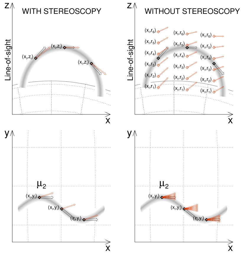
Figure 1: A diagram of the optimization parameters in the NLFFF forward-fitting method of the magnetic field to observed coronal loops is shown for the case of stereoscopic triangulation (left side), as well as for the case of 2D loop tracing without stereoscopy (right side). An observed loop (greyscale) is shown in the plane-of-sky $(x,y)$-plane (lower panels) and along the line-of-sight in the $(x,z)$-plane, as triangulated with stereoscopy. The black arrows demarcate the loop directions, while the red arrows indicate the field direction of the fitted magnetic field $B(x_{i},y_{i},z_{i})$ at loop positions $(x_{i},y_{i},z_{i})$. In the case without stereoscopy (right side), an array of field directions at altitudes $r_{1},...,r_{6}$ are calculated at projected loop positions $(x_{i},y_{i})$. The forward-fitting minimizes the misalignment angle $\mu_{2}$ between the field directions (red arrows) and the 2D loop directions (black arrows).

The two different methods are juxtaposed in Fig. 1. In the 3D forward-fitting method, the 3D misalignment angle $\mu_{3}(i,j),i=1,...,n_{s},j=1,...,n_{L}$ is computed for a number of $n_{s}$ loop segment positions and $n_{L}$ coronal loops, defined by the scalar product that calculates the angle $\mu_{3}$ between the 3D vectors of the loop direction ${\bf B}^{obs}({\bf x})$ and the magnetic field direction ${\bf B}^{theo}({\bf x})$ at a given loop position ${\bf x}(s)=[x(s_{ij}),y(s_{ij}),z(s_{ij})]$,

$$\mu_{3}({\bf x})=cos^{-1}\left({{\bf B}^{theo}({\bf x})\cdot{\bf B}^{obs}({\bf x})\over|{\bf B}^{theo}({\bf x})|\ |{\bf B}^{obs}({\bf x})|}\right)\ .$$ (9)

This is illustrated in Figure (1), where the loop directions (black arrows) and magnetic field directions (red arrows) are depicted at three loop segment positions, for two orthogonal projections (Figure 1 left panels). The root-mean-square value of all misalignment angles for each loop segment $(i)$ and loop $(j)$ is then minimized in the forward-fitting procedure to find the best NLFFF approximation,

$$\mu_{3}={1\over n_{s}n_{L}}\left(\sum_{i,j}^{n_{s},n_{L}}[\mu_{3}({\bf x}_{ij})]^{2}\right)^{1/2}\ .$$ (10)

In addition to the 3D misalignment angle $\mu_{3}$, we can also define a 2D misalignment angle $\mu_{2}$ with the same Equations (9) and (10), except that the magnetic field vectors ${\bf B}^{theo}({\bf x)}$ and loop vectors ${\bf B}^{theo}({\bf x})$ are a function of two-dimensional space coordinates ${\bf x}=(x_{ij},y_{ij})$, as they are seen in the 2D projection into the $(x,y)$-plane (Figure 1, bottom right panel).

If we have only 2D loop coordinates available (in the case without stereoscopy), we can only forward-fit the field lines parameterized with a NLFFF code by minimizing the 2D misalignment angle $\mu_{2}$, because the third space variable $(z_{ij})$ is not available. Our strategy here is to calculate the 2D misalignment angle $\mu_{2}$ in each position for an array of altitudes, $r_{i}=1+h_{max}(i/n_{h}),i=1,...,n_{h}$, that covers a limited altitude range $[1<r<(1+h_{max})]$ or search volume in which we expect coronal loops to be detectable (Figure 1, top right panel). For EUV images, loops are generally detectable within one density scale height, for which we use a height range of $[1<r<1.15]$ solar radii here. This yields multiple $(n_{h})$ misalignment angles for each 2D loop position $(x_{ij},y_{ij})$, which are shown in the $(x-z)$-plane (Fig. 1 top right panel) and $(x-y)$-plane (Fig. 1 bottom right panel). Our strategy is then to estimate the unknown third $z_{ij}$-coordinate in each 2D position $(x_{ij},y_{ij})$ from that height $r_{i}$ that shows the smallest 2D misalignment angle $\mu_{2}$, and can then proceed with the forward-fitting procedure like in the case of 3D stereoscopic data $(x_{ij},y_{ij},z_{ij})$, which is described in detail in Aschwanden and Malanushenko (2012).

A side-effect of the generalized 2D method is that the parameter space is enlarged by an additional dimension, i.e., the unknown $z_{i}$ or $r_{i}$ coordinate of the altitude of each loop position $(x_{ij},y_{ij})$, which in principle increases the computation time by a linear factor of the number $n_{h}$ of altitude levels. However, we optimized the code by vectorization and by organizing the optimization of the altitude variables $z_{ij}$ (for each loop segment $j$ and loop $i$) and the $\alpha_{k}$-parameter variables (for each magnetic charge $m$) in an interleaved mode, so that the computation time reduced by 1-2 orders of magnitude compared with earlier versions of the code (Aschwanden and Malanushenko 2012; Aschwanden et al., 2012a), without loss of accuracy.

When comparing 3D with 2D misalignment angles, we have to be aware that the unknown third dimension $z_{ij}$ at every loop position $(x_{ij},y_{ij})$ is handled differently in the two methods. In our new 2D method we optimize the third coordinate $z_{ij}$ by minimizing the 2D misalignment angle independently at every loop segment position $(x_{ij},y_{ij})$, interleaved with the optimization of the nonlinear force-free $\alpha_{m}$ parameter. In the (stereoscopic) 3D method the third coordinate $z_{ij}$ is used as a fixed constraint like the observables $(x_{ij},y_{ij})$. However, we can calculate the median 2D misalignment angle $\mu_{2}$ with both methods, while the 3D misalignment angle $\mu_{3}$ is only defined for the (stereoscopic) 3D-fit method, but not for the (loop-tracing) 2D-fit method.

4 TEST RUNS WITH SIMULATED DATA

In order to test the numerical convergence behavior, the uniqueness of the solutions, and the accuracy of the method in terms of misalignment angles we test our code first with simulated data. We simulate six cases that correspond to the same six nonpotential cases presented in Aschwanden and Malanushenko (2012; cases # 7-12), consisting of a unipolar case (N7; Figure 2 top), a dipolar case (N8; Figure 2 middle), a quadrupolar case (N9; Figure 2 bottom), and three decapolar cases with 10 randomly buried magnetic charges each (N10, N11, N12; Figure 3). In each case we run both the 3D-fitting code (mimicking the availability of stereoscopic loop data), as well as the 2D-fitting code (corresponding to loop tracings from a single EUV image without stereoscopic information). Thus, in the 3D-fitting code the target loops are parameterized with 3D data $[x_{i}(s),y_{i}(s),z_{i}(s)]$, while we ignore the third coordinate in the 2D-fitting code and fit only the 2D coordinates $[x_{i}(s),y_{i}(s)]$ of the target loops. The results are shown in Figures 2 and 3, with the 2D fits in the left-hand panels, and the 3D fits in the right-hand panels.

The convergence of the 2D-code can be judged by comparing with the previously tested 3D-code (Aschwanden and Malanushenko 2012). We list a summary of the results in Table 1. The 3D-fits achieve a mean 3D misalignment angle of $\mu_{3}=3.6^{\circ}\pm 1.9^{\circ}$ and a 2D misalignment angle of $\mu_{2}=2.0^{\circ}\pm 1.1^{\circ}$. This is reasonable and slightly better than the results of an earlier version of the 3D-code ($\mu_{3}=5.1^{\circ}\pm 4.3^{\circ}$ in Table 4 of Aschwanden and Malanushenko 2012). In comparison, our new 2D-fitting code achieves an even better agreement with $\mu_{2}=1.2^{\circ}\pm 0.5^{\circ}$ for the 2D-misalignment angle $\mu_{2}$, while the 3D-misalignment angle $\mu_{3}$ is not defined for the 2D code (due to the lack of line-of-sight coordinates $z$). The better performance of the 2D code is due to the smaller number of constraints (i.e., 200 constrains for 2D-loop coordinates of 10 loops with 10 segments, compared with 300 constraints for the 3D-fit method). The smaller number of free parameters generally improves the accuracy of the solution. The uniqueness of the solution can be best expressed by the mean misalignment angle $\mu_{2}$. Strictly speaking, a NLFFF solution would only be unique if the number of free parameters (i.e., the number of magnetic charges $N_{m}$ in our case) matches the number of constraints (i.e., the number of fitting positions (i.e., the product of the number of loops $N_{\rm loop}$ times the number of fitted segment positions $N_{segm}$, i.e., $N_{fit}=N_{loop}\times N_{seg}$ in our case). Moreover, the LOS magnetogram is approximated by a number of magnetic charges $N_{m}$ that neglects weak magnetic sources, and there are residuals in the decomposition of magnetic charges that contribute to the noise or uncertainty and non-uniqueness of the solutions. Therefore, the uniqueness of a NLFFF solution can best be specified by an uncertainty measure for each field line, which can be quantified either by the misalignment angle $\mu_{2}$ or by a maximum transverse displacement of a field line, i.e, $\Delta x\approx(L/2)\tan\mu_{2}$ for a particular field line with full length $L$.

We show in Table 1 also the ratios $E_{NP}/E_{P}$ of the nonpotential to the potential energies for the 3D and 2D fit methods, which agree within an accuracy of order $\approx 0.1-2.5\%$. Note, that the simulated data have 1, 2, 4, and 10 magnetic charges, which corresponds to the number of free parameters in the fit, while we used the double number of magnetic charges in the decomposition of the simulated LOS magnetogram, in order to make the parameterization of the fitted model somewhat different from the target model. Nevertheless, although the 2D solutions have a high accuracy (with a mean misalignment of $\mu_{2}=1.2^{\circ}\pm 0.5^{\circ}$), we have to be aware that the simulated data and the forward-fitting code use the same parameterization of nonlinear $\alpha$-parameters, which warrants a higher accurcay in forward-fitting than real data with a unknown parameterization. Hence, we test the code with real solar data in the following section.

5 OBSERVATIONS AND RESULTS

5.1 Observations

For testing the feasibility, fidelity, and accuracy of the new analytical NLFFF forward-fitting code based on 2D tracing of loops (rather than 3D stereoscopy) we are using the same observations for which either stereoscopic 3D reconstruction has been attempted earlier (Aschwanden et al., 2008b,c, 2009, 2012a; Sandman et al., 2009; DeRosa et al., 2009; Aschwanden and Sandman 2010; Sandman and Aschwanden 2011; Aschwanden 2012a), such as for active regions observed with STEREO on 2007 April 30, May 9, May 19, and December 11, or where 2D loop tracing was performed and documented, such as for an active region observed on 1998 May 19 with TRACE (Aschwanden et al., 2008a). The active region numbers, observing times, spacecraft separation angles, number of traced loops, and maximum magnetic field strengths of these observations are listed in Table 2. In all cases we used line-of-sight magnetograms $B_{z}(x,y,z_{phot})$ from the Michelson Doppler Imager (MDI; Scherrer et al., 1995) on board the Solar and Heliospheric Observatory (SOHO), while EUV images were used either from the Transition Region And Coronal Explorer (TRACE; Handy et al., 1999), or from the Extreme Ultraviolet Imager (EUVI; Wülser et al., 2004) onboard the STEREO spacecraft A(head) and B(ehind).

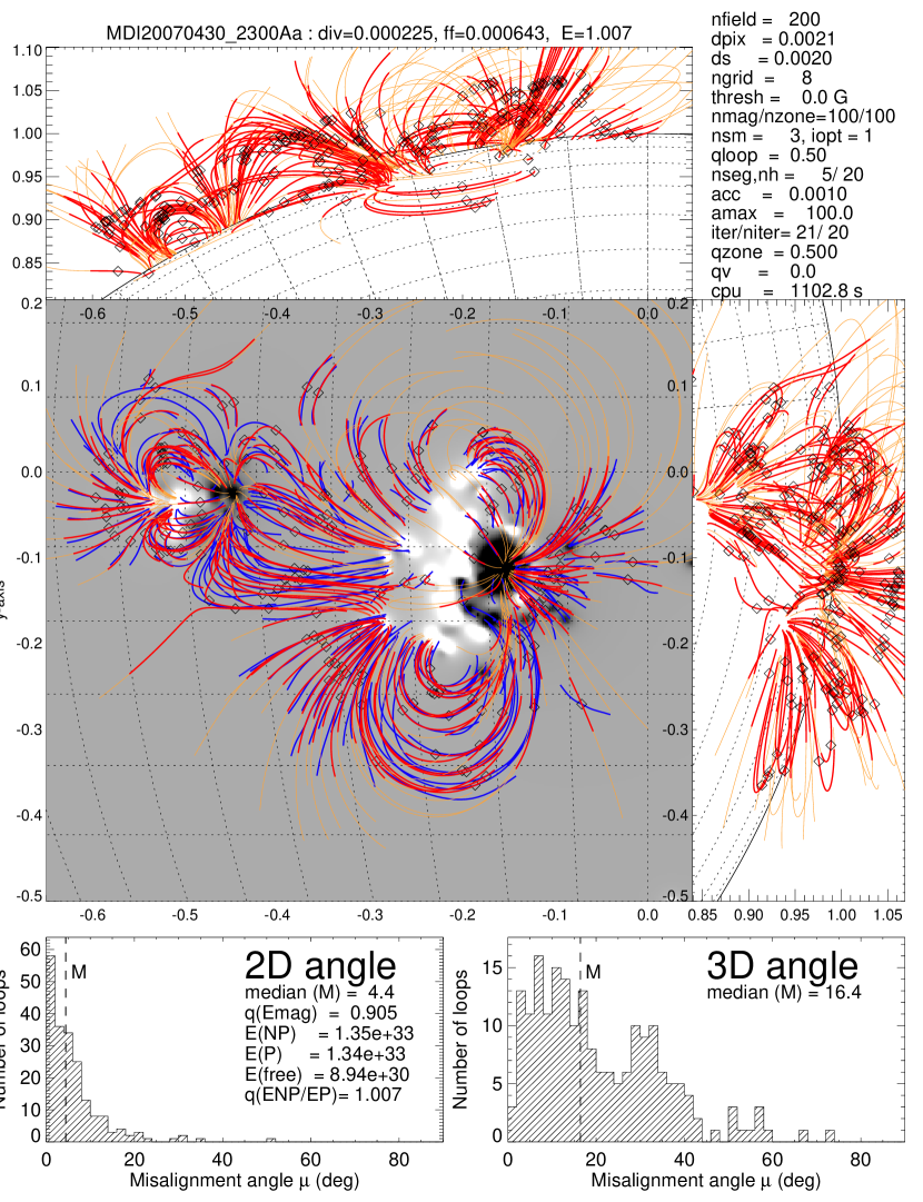
Figure 4: Forward-fitting of the NLFFF model to active region A (2007 April 30), using STEREO data: SoHO/MDI line-of-sight magnetogram (greyscale image), triangulated STEREO loops (blue curves), and best-fit magnetic field segments (red) with field line extensions (orange), shown in three orthogonal projections, and distribution of misalignment angles (bottom).

We show the results of the NLFFF forward-fitting of the six active regions in Figures 4 to 9, all in the same format, which includes the decomposed line-of-sight magnetogram of SoHO/MDI (grey scale in center of Figures 4 to 9), the stereoscopically triangulated or visually traced loops (blue curves in Figures 4 to 9), and the best-fit magnetic field lines (red curves for the segments covered by the observed loops, and in orange color for complementary loops parts (although truncated at a height of 0.15 solar radii). The orthogonal projections of the best-fit magnetic field lines are also shown in the right-hand and top panels of Figures 4 to 9, as well as the histograms of 2D $(\mu_{2})$ and 3D ($\mu_{3}$) misalignment angles (in bottom panels of Figures 4 to 9). The median misalignment angles $\mu_{2}$ and $\mu_{3}$ are also listed in Table 3, for both the previous stereoscopic reconstructions (Aschwanden et al., 2012a; Aschwanden 2012b), marked with ”STEREO” in Table 3, and based on 2D loop tracing in the present study, marked with ”Tracing” in Table 3.

The active region A (2007 April 30; Figure 4) shows a lack of stereoscopically triangulated loops in the core of the active region (due to the high level of confusion for loop tracing over the “mossy” regions), where the highest shear and degree of non-potentiality is expected, and thus deprives us from measuring the largest amount of free magnetic energy, while standard NLFFF codes have stronger constraints in these core regions. In all 5 active regions we see sunspots with strong magnetic fields, but since we limit our NLFFF solutions to an altitude range of $\lower 1.72218pt\hbox{$\;\buildrel<\over{\scriptstyle\sim}\;$}0.15$ solar radii, we cannot see whether the diverging field lines above the sunspots are open or closed field lines. In principle we could display our NLFFF solutions to larger altitudes to diagnose where open and closed field regions are, but the accuracy of reconstructed field lines is expected to decrease with height with our method, especially because of the second-order approximation that can represent helical twist well for vertical segments of loops (near the surface), but not so well for horizontal segments of loops (in large altitudes).

5.2 Misalignment Angle Statistics

We see in Table 3 that the 3D misalignment angles $\mu_{3}$ have a mean value of $\mu_{3}=19^{\circ}\pm 3^{\circ}$ for the stereoscopy method. If we compare the 2D misalignment angles $\mu_{2}$ between the two methods in Table 3, we see that the STEREO method has a somewhat larger mean, $\mu=4.0^{\circ}\pm 1.8^{\circ}$, than the 2D loop tracing method, with $\mu=2.7^{\circ}\pm 1.3^{\circ}$. This is an effect of the optimization of the 2D misalignment angles in the 2D loop tracing method, where the third coordinate is a free variable and thus has a larger flexibility to find an appropriate model field line with a small 2D misalignment angle, in contrast to the stereoscopic method, where the third coordinate of every observed loop is entirely fixed and leaves less room in the minimization of the misalignment angles between observed loops and theoretical field models. Ideally, if stereoscopy would work perfectly, the third coordinate should be sufficiently accurate so that the best field solution can be found easier with fewer free parameters. However, reality apparently reveals that there is a significant stereoscopic error that hinders optimum field fitting, which is non-existent in the 2D forward-fitting situation. Actually, from the two stereoscopic misalignment angles we can estimate the stereoscopic error $\sigma_{SE}$, assuming isotropic errors. Thus, defining the 2D misalignment angle as $\mu_{2}^{2}=\sigma_{x}^{2}+\sigma_{y}^{2}$, and the 3D misalignment angle as $\mu_{3}^{2}=\sigma_{x}^{2}+\sigma_{y}^{2}+\sigma_{z}^{2}+\sigma_{SE}^{2}$, with isotropic errors $\sigma_{x}=\sigma_{y}=\sigma_{z}$, we expect

$$\sigma_{SE}^{2}=\mu_{3}^{2}-\left({3\over 2}\right)\mu_{2}^{2}\ ,$$ (11)

which yields a stereoscopic error of $\sigma_{SE}\approx 20^{\circ}$. This is somewhat larger than estimated earlier from the parallelity of stereoscopically triangulated loops with close spatial proximity, which amounted to $\sigma_{SE}\approx 7^{\circ}=12^{\circ}$ (Aschwanden and Sandman 2010). Thus both estimates assess a substantial value to the stereoscopic error that exceeds the accuracy of the best-fit NLFFF solution based on 2D loop tracing ($\mu_{2}=2.7^{\circ}\pm 1.3^{\circ}$) by far. Nevertheless, both best-fit misalignment angles $\mu_{2}$ are consistent with each other for the two forward-fitting methods. This forward-fitting experiment thus demonstrates that we obtain equally accurate NLFFF fits to coronal data with or without stereoscopy, and thus makes the new method extremely useful.

5.3 Spatial Resolution of Instruments

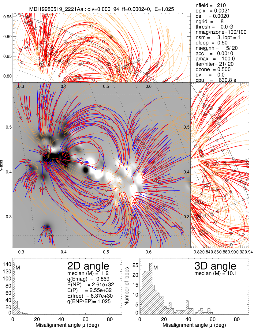
Figure 8: Forward-fitting of the NLFFF model to active region E (1998 May 19), using manually traced loops from TRACE data, in similar representation as Figure 4.

For the 2D loop tracing method of stereoscopic data (cases A, B, C, and D in Table 1) we just ignored information on the $z$-coordinate of loops in the 2D forward-fitting algorithm. For cases E and F, we compare visual tracing of loops (case E) with automated loop tracing (case F). Interestingly, we find the most accurate forward-fit for case E, which has a 2D misalignment error of only $\mu_{2}=1.2^{\circ}$ (Figure 8), which may have resulted from the higher spatial resolution of loop tracing using TRACE data (with a pixel size of $0.5\hbox{${}^{\prime\prime}$}$) in case E, compared with the three times lower resolution of STEREO (with a pixel size of $1.6\hbox{${}^{\prime\prime}$}$) in the cases A, B, C, and D.

5.4 Visual versus Automated Loop Detection

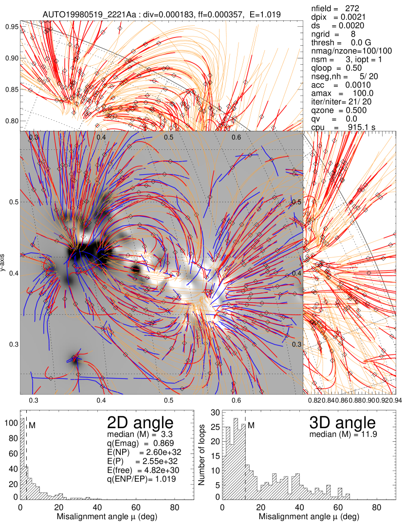
Figure 9: Forward-fitting of the NLFFF model to active region F (1998 May 19), using automatically traced loops from TRACE data, in similar representation as Figure 4.

Comparing visually traced (Figure 8) versus automatically traced loops (Figure 9), we note that the automated tracing leads to a less accurate NLFFF fit, with $\mu_{3}=3.3^{\circ}$ versus $\mu_{3}=1.2^{\circ}$ for visual tracing. Apparently, the automated loop tracing method (Aschwanden et al., 2008a) can easily be mis-guided or side-tracked by about $\Delta\mu\approx 2^{\circ}$ onto near-cospatial loops with similar coherent large curvature. Comparing individual field lines in Figure 8 with Figure 9, we see also that the automated loop tracing algorithm produces a number of short loop segments with large misalignment angles, which are obviously a weakness of the automated tracing code, resulting into a larger misalignment error for the fitted NLFFF solution (which is a factor of $\approx 3$ larger in the average for this case).

5.5 Magnetic Field Strengths

In Figure 10 we show scatterplots of the magnetic field strengths $B_{3}$ retrieved at the photospheric level for the stereoscopic 3D method versus the field strength $B_{2}$ obtained from the 2D loop tracing method. The analytical NLFFF forward-fitting algorithm starts first a decomposition of point-like buried magnetic charges from the line-of-sight component $B_{z}(x,y,z_{phot})$, but has no constraints for the transverse components $B_{x}$ and $B_{y}$, except for the coronal loop coordinates. Thus, the directions of coronal loops near the footpoints will determine the transverse components $B_{x}$ and $B_{y}$ in the photosphere. The scatterplots of $B_{2}$ versus $B_{3}$ in Figure 10 show that the smallest scatter between the two methods appears for active region B, which is the one closest to a potential field (although we are not able to trace and triangulate loops in the core of the active region, where supposedly the highest level of non-potentiality occurs). The linear regression fits show a good correspondence in the order of $\approx 0.1\%-1.0\%$ between the two methods, which results from different fitting criteria of the nonpotential field components. A ratio of $B_{\varphi}/B_{r}\approx 10\%$ in the azimuthal field (or nonpotential) field component $B_{\varphi}$ (Equation 5) with respect to the potential field component $B_{r}$ (Equation 4) would result into a change $B\approx\sqrt{(1+0.1^{2})}$ of $\approx 0.5\%$ in the magnetic field strength.

5.6 Magnetic Energies

The free magnetic energy, which is the difference between the nonpotential and the potential field energy, integrated over the spatial volume of an active region, has been calculated for the stereoscopic forward-fitting method in Aschwanden 2012b (Table 1 therein). Here we calculate these quantities also for the 2D loop tracing method, both methods being juxtaposed in Table 3 and in Figure 11. The absolute values of the potential field energy $E_{P}$ agree within a factor of $1.04\pm 0.02$ between the two methods, while the free energies show differences of 1%-2% of the potential energy. If we consider the difference in the free energy between two methods as a measure of a systematic error, we assess an uncertainty of $E_{free}/E_{P}-1=0.016\pm 0.013$, or about $\pm 1.5\%$.

6 DISCUSSION

6.1 Assessment of Various NLFFF Methods

Quantitative comparisons of various nonlinear force-free field (NLFFF) calculation methods applied to coronal volumes that encompass an active region included optimizational, magneto-frictional, Grad-Rubin based, and Green’s function based models (Schrijver et al., 2006; 2008; DeRosa et al., 2009). A critical assessment of 11 NLFFF methods revealed significant differences in the nonpotential magnetic energy and in the degree of misalignment ($\mu_{3}\approx 24^{\circ}-44^{\circ}$) with respect to stereoscopically triangulated coronal loops. The chief problem responsible for these discrepancies were identified in terms of the non-force-freeness of the lower (photospheric) boundary, too small boundary areas, and uncertainties of the boundary data (DeRosa et al., 2009). Obviously, the non-force-freeness of the photosphere can only be circumvented by incorporating coronal magnetic field geometries into NLFFF extrapolations, such as the information from stereoscopically triangulated loops.

Implementation of coronal magnetic field data into NLFFF codes is not straightforward, because most of the conventional NLFFF codes are designed to extrapolate from a lower boundary in upward direction, and thus the volume-filling coronal information cannot be treated as a boundary problem. A natural method to match arbitrary constraints that are not necessarily a boundary problem is a forward-fitting approach, which however, requires a parameterization of a magnetic field model. Since NLFFF models are implicitly defined by the two differential equations of force-freeness and divergence-freeness, an explicit parameterization of a magnetic field is not trivial. There are essentially three approaches that have been attempted so far: (i) Preprocessing of magnetic boundary data by minimizing the Lorentz force at multiple spatial scales (Wiegelmann 2004; Jing et al., 2009); (ii) linear force-free fitting with subsequent relaxation to a nonlinear force-free field (Malanushenko et al., 2009, 2012); and (iii) magnetic field parameterization with buried magnetic charges and forward-fitting of an approximative analytical NLFFF solution (Aschwanden 2012a,b; Aschwanden and Malanushenko 2012). The third method requires stereoscopically triangulated 3D coordinates of coronal loops, which have been successfully modeled in four different active regions, improving the misalignment angles between the observed loops and a potential field ($\mu_{3}=19^{\circ}-46^{\circ}$) by a factor of about two, when fitted with the analytical NLFFF solution ($\mu_{3}=14^{\circ}-19^{\circ}$; Aschwanden et al., 2012a). However, although this method provides a more realistic NLFFF model, the main restriction is the availability of STEREO data, as well as the inferior spatial resolution of STEREO/EUVI compared with other EUV imagers (e.g., TRACE, or SDO/AIA). In order to circumvent this restriction we developed a generalized code in this study that requires only a high-resolution EUV image, from which a sufficient large number of coronal loops can be traced in two dimensions, plus a line-of-sight magnetogram, which were essentially always available since the lauch of the SOHO mission in 1995. A fortunate outcome of this study is that the reduction of 3D information from coronal loops to 2D coordinates does not handicap the accuracy of a NLFFF forward-fitting method, as we demonstrated here. One potential limitation of forward-fitting of analytical NLFFF approximations may be the accuracy for strong nonpotential cases (say near flaring times), since our analytical NLFFF approximation is only accurate to second order of the force-free $\alpha$-parameter. Another caveat may be the universality of the analytical NLFFF parameterization. Our approximation is designed to model azimuthal (rotational) twist around a vertical axis with respect to the solar surface, which corresponds to electric currents flowing in vertical direction. This geometry may not be appropriate for horizontally twisted structures, such as horizontally extended filaments. For such cases, a more general NLFFF solution could be desirable. In this respect, more general NLFFF solutions such as currently developed by Malanushenko et al., (2009; 2012) may provide new tools, after they will be generalized for a spherical solar surface and optimized for computational speed. Nevertheless, our analytical NLFFF forward-fitting algorithm can always be used to find a quick first approximation of a NLFFF solution, which then could be refined by alternative (more time-consuming) NLFFF codes.

6.2 Computational speed

Note that our forward-fitting code calculates one trial magnetic field configuration in about 0.01 s, while some $10^{4}-10^{5}$ iterations are needed for the convergence of an approximate NLFFF solution, accumulating to a few minutes total computation time. Our forward-fitting code computes a solution to an active region with an average computation time of $\approx 10$ minutes (see CPU times in Table 3) on a Mac OS X, 2 $\times$ 3.2 GHz Quad-Core Intel Xeon, 32 GB memory, 800 MHz DDR2 FB-DIMM computer. Simple cases that can be represented with $N)m\lower 1.72218pt\hbox{$\;\buildrel<\over{\scriptstyle\sim}\;$}20$ magnetic charges, require only computation times of order $\lower 1.72218pt\hbox{$\;\buildrel<\over{\scriptstyle\sim}\;$}10$ s (see CPU times in Table 1).

7 CONCLUSIONS

We developed an analytical NLFFF forward-fitting code that requires only the input of a line-of-sight magnetogram $B_{z}(x,y,z_{phot})$ and a set of 2D loop tracing coordinates $(x_{i},y_{i})$ that can be obtained from any high-resolution EUV image. This is the first attempt to measure the coronal magnetic field based on directly observed 2D images alone, while we needed stereoscopically triangulated 3D loop coordinates $(x_{i},y_{i},z_{i})$ from STEREO in previous studies. There exists only one other study (to our knowledge) that heads into the same direction of forward-fitting a NLFFF model to 2D data (Malanushenko et al., 2012), using simulated 2D data based on analytical NLFFF solutions (from Low and Lou 1990) or previous NLFFF modeling (from Schrijver et al., 2008).

We forward-fitted analytical NLFFF approximations to four active regions (cases A, B, C, D) using 2D loop tracings only and compared them with previous NLFFF fits using (stereoscopic) 3D loop coordinates. Furthermore we forward-fitted analytical NLFFF approximations to another active region using visual 2D loop tracings (case E) or automatically traced 2D loop coordinates (case F). Our findings of these exercises are the following:

1. Our forward-fitting experiment with two different methods demonstrated that a nonlinear force-free magnetic field (NLFFF) solution ${\bf B}({\bf x})$ can be obtained with equal accuracy with or without stereoscopy. This result relinquishes the necessity of STEREO data for future magnetic modeling of active regions on the solar disk, but the availability of suitable STEREO data was crucial to establish this result.

2. The accuracy of a forward-fitted NLFFF approximation that includes vertical currents (with twisted azimuthal magnetic field components) matches coronal loops observed in EUV with a median 2D misalignment angle of $\mu_{2}=2.7^{\circ}\pm 1.3^{\circ}$, while stereoscopic 3D data exhibit a commensurable 2D misalignment angle, but a substantially larger 3D misalignment angle ($\mu_{3}=19^{\circ}\pm 3^{\circ}$), which implies stereoscopic measurement errors in the order of $\sigma_{SE}\approx 20^{\circ}$. These substantial stereoscopic measurement errors lead to less accurate NLFFF fits than 2D loop tracings with unconstrained line-of-sight positions.

3. 2D loop tracings in high resolution images (i.e., $0.5\hbox{${}^{\prime\prime}$}$ pixels with TRACE) lead to more accurate NLFFF fits (with a misalignment angle of $\mu_{2}=1.2^{\circ}$ in case E) than images with lower spatial resolution (i.e., $1.6\hbox{${}^{\prime\prime}$}$ pixels with STEREO), yielding $\mu_{2}=4.0^{\circ}\pm 1.8^{\circ}$ for the cases A, B, C, and D.

4. Visually (or manually) traced 2D loop coordinates appear to be still superior to the best automated loop tracing algorithms, yielding a misalignment angle of $\mu_{2}=1.2^{\circ}$ (in case E) versus $\mu_{2}=3.3^{\circ}$ (in case F).

5. Magnetic field strengths $B$ of best-fit NLFFF approximations are retrieved with an accuracy of $\approx 0.1\%-1.0\%$, comparing the 2D loop tracing method with the stereoscopic 3D triangulation method.

6. Magnetic energies differ by a factor of $\approx 4\%\pm 2\%$ between the two methods, while the free energy has a systematic error of $\approx\pm 1.5\%$ (of the total magnetic energy) between the two methods, which is about an order of magnitude smaller than found between other (standard) NLFFF codes.

7. The computational speed of our NLFFF code allows the computation of a space-filling magnetic field configuration of an active region in about 0.01 s, while forward-fitting to a set of coronal loops is feasible with about $10^{4}-10^{5}$ iterations, requiring a total computation time of a few minutes.

These results demonstrate clearly that we can perform accurate NLFFF magnetic modeling based on 2D loop tracings, which will relinquish the need of STEREO data in future, at least for active regions near the solar disk center. The analyzed active regions extended up to 0.65 solar radii away from disk center, so in principle we can perform NLFFF modeling for at least half of the number of active regions observed on the solar disk, especially since the parameterization of our analytical NLFFF approximation takes the sphericity of the solar surface fully into account (which is not the case in most other NLFFF codes). For future developments we expect that other NLFFF codes could implement minimization of the misalignment angle $\mu_{2}$ with coronal loops in parallel to the optimization of force-freeness and divergence-freeness, rather than by preprocessing of vector boundary data. Further improvements in automated 2D loop tracings could replace visual/manual tracing methods and this way render NLFFF modeling with coronal constraints in a fully automated way.

Table 1: Median 2D and 3D misalignment angles $\mu_{2}$ and $\mu_{3}$ and free energy ratios $E_{NP}/E_{P}$ for six simulated magnetic field configurations (see Figures 2 and 3), using the 3D-fit code suitable for stereoscopic data (marked with ”STEREO”), and using the 2D-fit code suitable for 2D loop data (marked with ”Tracing”). The computation time (CPU) is listed in seconds.

Data set	CPU (s)	STEREO	STEREO	Tracing	STEREO	Tracing
		$\mu_{3}$	$\mu_{2}$	$\mu_{2}$	$E_{NP}/E_{P}$	$E_{NP}/E_{P}$
N7	0.3	$0.6^{\circ}$	$0.1^{\circ}$	$0.7^{\circ}$	1.009	1.034
N8	2.1	$2.2^{\circ}$	$1.4^{\circ}$	$0.6^{\circ}$	1.010	1.009
N9	3.0	$3.7^{\circ}$	$2.4^{\circ}$	$1.4^{\circ}$	1.016	1.015
N10	16.5	$5.0^{\circ}$	$3.2^{\circ}$	$1.6^{\circ}$	1.055	1.054
N11	12.5	$5.5^{\circ}$	$2.2^{\circ}$	$1.8^{\circ}$	1.066	1.050
N12	17.8	$4.6^{\circ}$	$2.4^{\circ}$	$1.1^{\circ}$	1.140	1.094
Mean	$8.7\pm 7.8$	$3.6\pm 1.9$	$2.0\pm 1.1$	$1.2\pm 0.5$

Table 2: Data selection of four Active Regions observed with SOHO/MDI and STEREO/EUVI or TRACE.

Case	Active	Observing	Observing	Observing	Spacecraft	Number	Magnetic
	Region	date	time EUV	time MDI	separation	of EUVI	field strength
			(UT)	(UT)	angle (deg)	loops	B(G)
A	10953 (S05E20)	2007-Apr-30	23:00-23:20	22:24	STEREO 6.0∘	200	[-3134,+1425]
B	10955 (S09E24)	2007-May-9	20:30-20:50	20:47	STEREO 7.1∘	70	[-2396,+1926]
C	10953 (N03W03)	2007-May-19	12:40-13:00	12:47	STEREO 8.6∘	100	[-2056,+2307]
D	10978 (S09E06)	2007-Dec-11	16:30-16:50	14:23	STEREO 42.7∘	87	[-2270,+2037]
E	8222 (N22W30)	1998-May-19	22:21-22:22	20:48	TRACE (manu)	201	[-1787,+1200]
F	8222 (N22W30)	1998-May-19	22:21-22:22	20:48	TRACE (auto)	222	[-1787,+1200]

Table 3: Median 2D and 3D misalignment angles $\mu_{2}$ and $\mu_{3}$ and free energy ratios $E_{NP}/E_{P}$ for six active regions, including four stereoscopically triangulated loops observed with STEREO (A-D) and two cases with traced loops observed with TRACE (E-F). All cases have also been modeled by forward-fitting of the NLFFF model to the traced 2D loop coordinates (columns marked with “Tracing”). The computation time (CPU) is listed in seconds.

Data set	CPU (s)	STEREO	STEREO	Tracing	STEREO	Tracing
		$\mu_{3}$	$\mu_{2}$	$\mu_{2}$	$E_{NP}/E_{P}$	$E_{NP}/E_{P}$
A) 2007-Apr-30	1103	$21.4^{\circ}$	$4.6^{\circ}$	$4.4^{\circ}$	1.006	1.007
B) 2007-May-9	208	$17.9^{\circ}$	$3.7^{\circ}$	$2.4^{\circ}$	1.023	1.009
C) 2007-May-19	415	$22.1^{\circ}$	$5.9^{\circ}$	$3.6^{\circ}$	1.085	1.053
D) 2007-Dec-11	390	$14.7^{\circ}$	$1.6^{\circ}$	$1.5^{\circ}$	1.044	1.026
E) 1998-May-19 (manu)	631			$1.2^{\circ}$
F) 1998-May-19 (auto)	915			$3.3^{\circ}$
(A-F) Mean	$610\pm 342$	$19^{\circ}\pm 3^{\circ}$	$4.0^{\circ}\pm 1.8^{\circ}$	$2.7^{\circ}\pm 1.3^{\circ}$

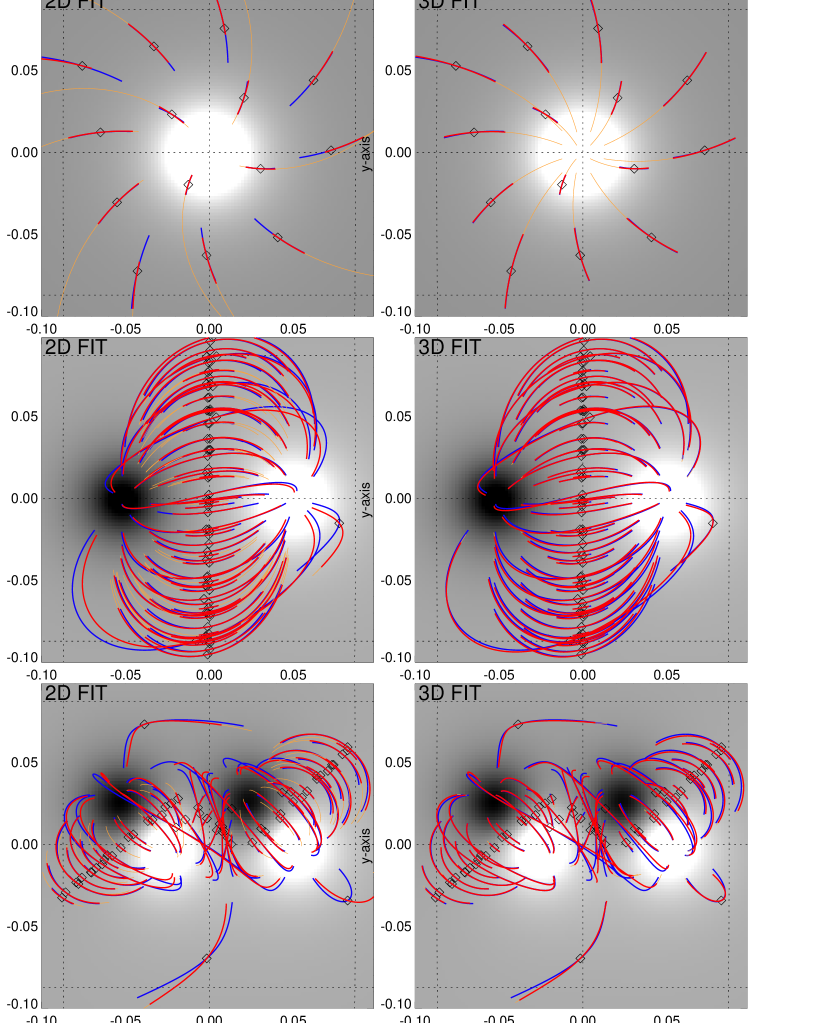
Figure 2: Forward-fitting of the NLFFF model to simulated data of a unipolar (top; case N7), a dipolar (middle; case N8), and quadrupolar magnetic configuration (bottom; Case N9), using the 2D-coordinates of simulated loops only (left panels) or the full 3D-coordinates of the simulated loops (right panels). The blue curves indicate the target loops, the red curves the best-fit field lines, and the grey-scale the simulated line-of-sight magnetogram. The cases N7, N8, and N9 are identical to the simulated cases shown in Figure (2) of Aschwanden (2012).

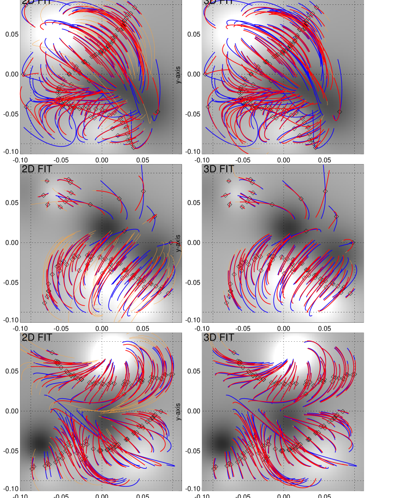
Figure 3: Forward-fitting of the NLFFF model to three simulated data cases with decapolar magnetic configurations (Cases N10, N11, N12, which are identical to the cases shown in Figure (3) of Aschwanden, 2012), using the 2D-coordinates of simulated loops only (left panels) or the full 3D-coordinates of the simulated loops (right panels). The blue curves indicate the target loops, the red curves the best-fit field lines, and the grey-scale the simulated line-of-sight magnetograms.

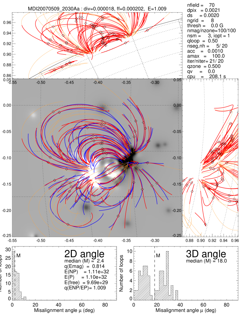
Figure 5: Forward-fitting of the NLFFF model to active region B (2007 May 9), using STEREO data, in similar representation as Figure 4.

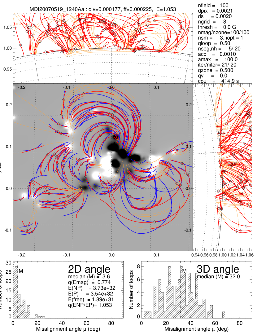
Figure 6: Forward-fitting of the NLFFF model to active region C (2007 May 19), using STEREO data, in similar representation as Figure 4.

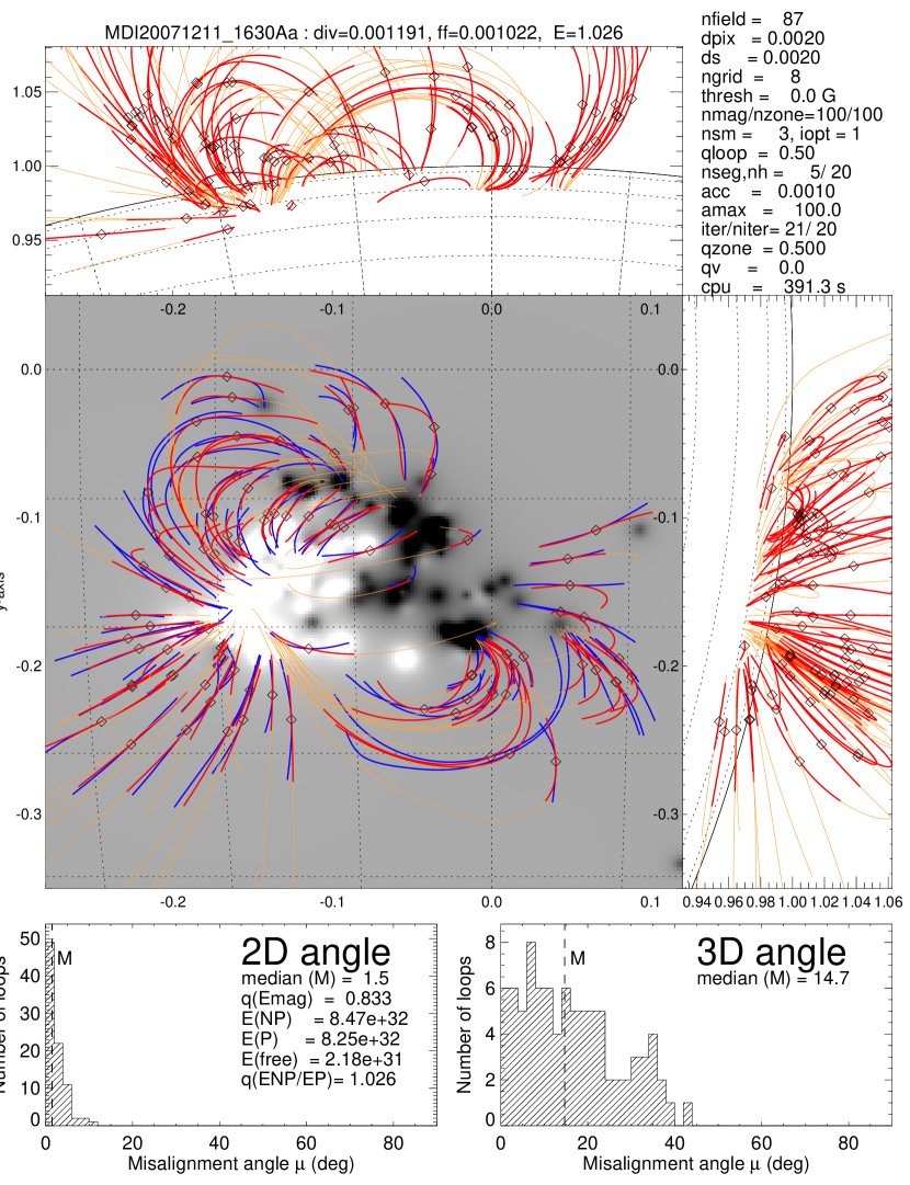
Figure 7: Forward-fitting of the NLFFF model to active region D (2007 Dec 11), using STEREO data, in similar representation as Figure 4.

Figure 10: Magnetic field strength $B(x,y,z=1)$ in a plane tangential to solar surface (at $z=1.0$ solar radii from Sun center), calculated from NLFFF fitting to stereoscopic data (x-axis) versus fitting to 2D loop tracing data (y-axis). Each scatterplot contains the datapoints from a field-of-view that encompasses the full EW extent and the middle 10% of the NS extent shown in Figures 4 to 9.

Figure 11: Nonpotential magnetic energy (top panel) and ratio of nonpotential to potential energy (bottom) integrated over each active region (A, B, C, D) over a height range of $\Delta h=0.015$ solar radii above the photosphere and a field-of-view as shown in Figures 4 to 9.

References

- (1)
- (2) Amari, T., Boulmezaoud, T.Z. and Mikic,Z., 1999, A&A350, 1051.
- (3) Amari, T., Boulmezaoud, T.Z., and Aly, J.J., 2006, A&A, 446, 691.
- (4) Aschwanden,M.J., Lee,J.K., Gary,G.A., Smith,M., and Inhester,B. 2008a, Sol. Phys., 248, 359.
- (5) Aschwanden, M.J., Wuelser, J.P., Nitta, N.V., and Lemen, J.R. 2008b, ApJ, 679, 827.
- (6) Aschwanden, M.J., Nitta, N.V., Wuelser, J.P., and Lemen, J.R. 2008c, ApJ, 680, 1477.
- (7) Aschwanden, M.J., Wuelser, J.P., Nitta, N., Lemen, J., and Sandman, A. 2009, ApJ, 695, 12.
- (8) Aschwanden, M.J. and Sandman, A.W. 2010, Astronomical J. 140, 723.
- (9) Aschwanden, M.J. 2011, Living Reviews in Solar Physics 8, 5.
- (10) Aschwanden,M.J. 2012a, Sol. Phys., online-first, DOI 10.1007/s11207-012-0069-7.
- (11) Aschwanden,M.J. and Malanushenko, A. 2012, Sol. Phys., online-first.
- (12) Aschwanden, M.J., Wuelser, J.P., Nitta, N., Lemen, J., Schrijver, C.J. DeRosa, M., and Malanushenko, A., 2012a, ApJ, 756, 124.
- (13) Aschwanden, M.J., 2012b, Sol. Phys., (in press).
- (14) Aschwanden, M.J., Wuelser, J.P., Nitta, N.V., and Lemen, J.R., 2012b, Sol. Phys., 281, 101.
- (15) Conlon, P.A. and Gallagher, P.T., 2010, ApJ, 715, 59.
- (16) DeRosa, M.L., Schrijver, C.J., Barnes, G., Leka, K.D., Lites, B.W., Aschwanden, M.J., Amari, T., Canou, A., McTiernan, J.M., Regnier, S., Thalmann, J., Valori, G., Wheatland, M.S., Wiegelmann, T., Cheung, M.C.M., Conlon, P.A., Fuhrmann, M., Inhester, B., and Tadesse, T. 2009, ApJ, 696, 1780.
- (17) Feng, L., Wiegelmann, T., Inhester, B., Solanki, S., Gan, W. Q., and Ruan, P., 2007, Sol. Phys., 241, 235.
- (18) Gold, T. and Hoyle,F. 1960, MNRAS 120/2, 89.
- (19) Grad, H., Rubin, H., 1958, Proc. 2nd UN Int. Conf. Peaceful Uses of Atomic Energy, 31, 190.
- (20) Handy, B. et al., 1999, Sol. Phys., 187, 229.
- (21) Inhester, B. 2006, ArXiv e-print: astro-ph/0612649.
- (22) Inhester, B., Feng,L., and Wiegelmann,T., 2008, Sol. Phys., 248, 379.
- (23) Jing, J., Tan,C., Yuan, Y., Wang, B., Wiegelmann, T., Xu,Y., Wang H., 2010, ApJ, 713, 440.
- (24) Low, B.C., and Lou, Y.Q., 1990, ApJ, 408, 689.
- (25) Malanushenko, A., Longcope, D.W., and McKenzie, D.E., 2009, ApJ, 707, 1044.
- (26) Malanushenko, A., Schrijver, C.J., DeRosa, M.L., Wheatland, M.S., Gilchrist, S.A., 2012, ApJ, 756, 153.
- (27) Metcalf, T.R., Jiao, L., Uitenbroek, H., McClymont, A.N., Canfield,R.C. 1995, ApJ, 439, 474.
- (28) Sandman, A., Aschwanden, M.J., DeRosa, M., Wuelser, J.P. and Alexander, D. 2009, Sol. Phys., 259, 1.
- (29) Sandman, A.W. and Aschwanden, M.J. 2011, Sol. Phys., 270, 503.
- (30) Scherrer, P.H., et al., 1995, Sol. Phys., 162, 129.
- (31) Schrijver, C.J., DeRosa, M., Metcalf, T.R., Liu, Y., McTiernan, J., Regnier, S., Valori, G., Wheatland, M.S., and Wiegelmann, T. 2006, Sol. Phys., 235, 161.
- (32) Schrijver, C.J., DeRosa, M., Metcalf, T.R., Barnes, G., Lites, B., Tarbell, T., McTiernan, J., Valori, G., Wiegelmann, T., Wheatland, M.S., Amari, T., Aulanier, G., Demoulin, P., Fuhrmann, M., Kusano, K., Regnier, S., and Thalmann J.K., 2008, ApJ, 675, 1637.
- (33) Valori, G., Kliem, B., and Fuhrmann, M., 2007, Sol. Phys., 245, 263.
- (34) Wheatland, M.S., Sturrock, P.A., Roumeliotis, G. 2000, ApJ, 540, 1150.
- (35) Wheatland, M.S., 2006, Sol. Phys., 238, 29.
- (36) Wheatland, M.S. and Regnier, S., 2009, ApJ700, L88.
- (37) Wiegelmann, T., 2004, Sol. Phys., 219, 87.
- (38) Wiegelmann, T., Inhester, B., and Feng, L. 2009, Annales Geophysicae 27/7, 2925.
- (39) Wiegelmann, T. and Sakurai T. 2012, Living Rev. Solar Phys., 9, 5.
- (40) Wülser J.P. et al., 2004, SPIE, 5171, 111.
- (41) Yang, W.H., Sturrock, P.A., and Antiochos, S.K., 1986, ApJ, 309, 383.