Impurity-induced frustration: low-energy model of diluted oxides

Abstract

We provide a detailed derivation of the low-energy model for Zn-diluted La₂CuO₄ in the limit of low doping together with a study of the ground-state properties of that model. We consider Zn-doped La₂CuO₄ within a framework of the three-band Hubbard model, which closely describes high-$T_{c}$ cuprates on the energy scale of the most relevant atomic orbitals. To obtain the low-energy effective model, we first determine hybridized electronic states of CuO₄ and ZnO₄ plaquets within the CuO₂ planes. Qualitatively, we find that the hybridization of zinc and oxygen orbitals can result in an impurity state with the energy $\varepsilon$, which is lower than the effective Hubbard gap $U$. In the limit of the effective hopping integral $t\ll\varepsilon$, $U$, the low-energy, spin-only Hamiltonian includes terms of the order $t^{2}/U$ and $t^{4}/\varepsilon^{3}$. That is, besides the usual nearest-neighbor superexchange $J$-terms of order $t^{2}/U$, the low-energy model contains impurity-mediated, further-neighbor frustrating interactions among the Cu spins surrounding Zn-sites in an otherwise unfrustrated antiferromagnetic background. These terms, denoted as $J^{\prime}_{\rm Zn}$ and $J^{\prime\prime}_{\rm Zn}$, are of order $t^{4}/\varepsilon^{3}$ and can be substantial when $\varepsilon\sim U/2$, the latter value corresponding to the realistic CuO₂ parameters. In order to verify this spin-only model, we subsequently apply the $T$-matrix approach to study the effect of impurities on the antiferromagnetic order parameter. Previous theoretical studies, which include only the dilution effect of impurities, show a large discrepancy with experimental data in the doping dependence of the staggered magnetization at low doping. We demonstrate that this discrepancy is eliminated by including impurity-induced frustrations into the effective spin model with realistic CuO₂ parameters. Recent experimental study shows a significantly stronger suppression of spin stiffness in the case of Zn-doped La₂CuO₄ compared to the Mg-doped case and thus gives a strong support to our theory. We argue that the proposed impurity-induced frustrations should be important in other strongly correlated oxides and charge-transfer insulators.

I Introduction

Impurity effects in spin systems have attracted considerable attention since the 1960s as a part of the broader interest in defects in solidsIzyumov_66 ; Jones71 ; AG59 ; Villain_79 and also in the context of percolative phenomena,Breed_70 ; Harris_77 ; Stinchcombe ; Cowley_77 to which diluted magnets provide excellent experimental realizations. More recently, the discovery of high-$T_{c}$ superconductivity in insulating antiferromagnets doped by mobile charge carriers has lead to an extensive research effort in various aspects of the problem, including role of disorder in quantum critical states,Vojta quantum percolation,Sandvik02 ; Greven_MC and others. It has also been realized that impurities may serve as valuable local probes into the properties of strongly correlated systems in general, revealing important aspects of their electronic degrees of freedom.Vershinin ; Balatsky

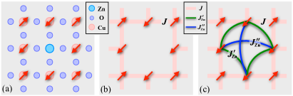
Figure 1: (Color online) (a) A schematic view of Zn-doped CuO₂ plane. (b) Site-diluted Heisenberg model representation of it. The arrows are Cu spins and the lines denote superexchange interactions. (c) The same, with extra frustrating interactions between the next- ($J^{\prime}_{\rm{Zn}}$) and the next-next- ($J^{\prime\prime}_{\rm{Zn}}$) nearest neighbor Cu sites, surrounding Zn impurity.

Out of the parent compounds of cuprate superconductors, it is La₂CuO₄ that has been studied most comprehensively.cuprates ; Xiao_90 ; Cheong_91 ; Corti_95 ; Carretta_97 ; Buchner_99 ; Greven_02 ; Greven_03 In its pristine form, it is an excellent realization of the two-dimensional, spin-$\frac{1}{2}$, nearest-neighbor square-lattice Heisenberg antiferromagnetManousakis_91 ; Dagotto_94 ; Chakravarty_89 formed by Cu²⁺ ions surrounded by oxygens. The dilution is achieved by chemically substituting isovalent Zn²⁺ or Mg²⁺ spinless ions for Cu²⁺, see Fig. 1(a). Thus, it is only natural to expect that the proper low-energy model of La₂Cu_1-x(Zn,Mg)_xO₄ must be the nearest-neighbor site-diluted Heisenberg model,Greven_02 ; Greven_03 see Fig. 1(b). In order to elucidate the properties of La₂CuO₄ diluted by spinless impurities, and of the associated site-diluted spin model, extensive experimental studies have been performed using nuclear magnetic resonance (NMR) [nuclear quadrupole resonance (NQR)], muon spin relaxation ($\mu$SR), elastic and inelastic neutron scattering, and magnetometry.Cheong_91 ; Greven_03 ; Greven_02 ; Corti_95 ; Carretta_97 An equally comprehensive theoretical effort included the spin-wave $T$-matrix, Quantum Monte Carlo, and numerical real-space $1/S$ calculations of a number of quantities that allowed for extensive cross-examinations.Bulut ; kampf ; Mahan ; Wan ; NN ; Sandvik ; KK_imp ; Yasuda ; Chernyshev_01 ; Chernyshev_02 ; Sandvik02a ; Kato ; Mucciolo ; Delannoy_09

One quantity in particular, the average magnetic moment per Cu, $M(x)$, has been investigated in detail. The doping dependence of $M(x)$ is the purely quantum effect related to the impurity-induced suppression of the order parameter because the normalization to the number of magnetic ions naturally separates the classical effect of dilution from it. While the overall results for $M$ vs $x$ show a reasonable agreement, a substantial discrepancy between the experiment and the theory, both analytical and QMC, has been observed. The experimental results indicate a substantially stronger—a factor of approximately 2—suppression of the order parameter $M$ per impurity due to disorder-induced quantum fluctuations, and the experimental data for $M(x)$ are also always below the theoretical curves.Greven_02 ; Delannoy_09

In our recent work,Liu_09 a resolution to this problem has been suggested: impurities should not be considered as electronically inert vacancies that simply eliminate interactions among surrounding Cu spins. In addition to the dilution, the hybridized electronic states of the impurity and of the nearest oxygens can provide extra degrees of freedom that generate longer-range frustrating interactions, schematically shown in Fig. 1(c). Such impurity-induced frustrating interactions can be expected to significantly enhance local quantum fluctuations. In Ref. Liu_09, we have outlined our approach to the problem and presented our results for $M(x)$ together with the complementary QMC results. The latter have unequivocally supported the same conclusion: the dilution-frustration model exhibits stronger suppression of the order and, for a choice of parameters appropriate for Zn-doped La₂CuO₄, bridges the gap between experiments and previous theoretical calculations based on the dilution-only model. Since then our theory has received further experimental confirmation from the $\mu$SR studies of spin stiffness in Zn and Mg doped La₂CuO₄,Carretta_11 which demonstrated a stronger suppression of spin stiffness in Zn-doped case, in agreement with the expectations from the theory.

In this work, we expose the details of the derivations of the dilution-frustration model and of the subsequent analytical calculations of the doping-dependent magnetization. The key element of our theory is that it starts from a realistic model, the site-diluted three-band Hubbard model, instead of already “effective” models of the CuO₂ plane, such as the diluted Heisenberg or the diluted one-band Hubbard model.

We begin with Zn-doped La₂CuO₄ within the framework of the impurity-doped three-band Hubbard model, which closely describes the diluted high-$T_{c}$ cuprates and other transition-metal oxides on the energy scale of the most relevant atomic orbitals.Emery ; ER Similar to the derivation of the one-band Hubbard model from the three-band Hubbard model,ZR ; Jefferson_92 the cell-perturbation approach is used to describe hybridization of the energy levels of Cu and Zn with oxygen orbitals. The approach does not require Cu-O and Zn-O hopping integrals to be smaller than the charge-transfer gap, therefore the locally hybridized states on Cu or Zn and surrounding O’s are diagonalized without approximation.Jefferson_92 ; Chernyshev_93 ; Chernyshev_94_01 ; Chernyshev_94_02 ; Chernyshev_96 Then the three-band model can be rewritten as a “multi-orbital” Hubbard model with the effective “Cu” and “Zn” states connected by effective hoppings. Since the structure of the lowest states in the single-particle and two-particle sectors of the multi-orbital model is the same as in the one-band Hubbard model (i.e. the lowest two-hole state is the Zhang-Rice-like singlet), the equivalence of the two models can be justified.Jefferson_92 ; Chernyshev_93 ; Chernyshev_94_01 ; Chernyshev_94_02 In this approach, for the dilution-only picture to be valid the effective “Zn”-states must not occur below the effective Hubbard $U$, the situation more likely to be valid for the case of Mg-doping due to the lack of available electronic states on Mg ion. For the case of Zn-doping, its electronic statesCheng_05 ; Xiang ; Plakida hybridize with the states on the oxygen orbitals and can result in the states below the Hubbard energy gap. This provides surrounding Cu-spins with additional virtual states to execute their superexchange processes through, thus facilitating extra couplings that connect spins in the immediate vicinity of impurity. Therefore, the spinless impurity, in effect, can lead to a cage of frustrating interactions around itself, shown in Fig. 1(c).

For the sake of a qualitative picture, and in the spirit of mapping of the multi-band Hubbard model onto the single-band one, the result of this consideration is that the impurity-doped system is not equivalent to the site-diluted Hubbard model with electronically inert impurity sites, but rather to the $t$-$\varepsilon$-$U$ model, where in addition to the usual hopping $t$ and the two-particle energy gap $U$ there is the lowest energy state of the effective impurity sector, denoted as $\varepsilon$. At half-filling, the $t$-$U$ part reduces to the Heisenberg model with $J\!\sim\!t^{2}/U$, as usual, with the higher-order terms $\sim\!t^{4}/U^{3}$ negligible if $t\!\ll\!U$.Takahashi_77 ; Yoshioka_88 ; Chernyshev_04 Virtual transitions through the effective impurity level $\varepsilon$ generate superexchange interactions of the order of $t^{4}/\varepsilon^{3}$ between the next- and the next-next-nearest-neighbor Cu-spins ($J^{\prime}_{\rm Zn}$ and $J^{\prime\prime}_{\rm Zn}$) that are also nearest-neighbors of the impurity site. When the energy at the impurity site $\varepsilon$ is less than the Hubbard gap, such terms are not negligible and may be comparable to $J$. For an estimate, taking $\varepsilon=U/2$ and $U/t=10$ gives $J^{\prime}_{\rm Zn}/J\!\sim\!(t/U)^{2}(U/\varepsilon)^{3}\!\sim\!0.1$, and, given the geometry of the square lattice, the combined effect per impurity is $J^{tot}_{\rm Zn}\!=\!4J^{\prime}_{\rm Zn}\!+\!2J^{\prime\prime}_{\rm Zn}\!\sim\!0.6J$. The origin of $J^{\prime}_{\rm Zn}$ and $J^{\prime\prime}_{\rm Zn}$ is clearly distinct from the generally considered next- and next-next-nearest-neighbor superexchange interaction ($J_{2}$ and $J_{3}$), which are of the order of $t^{4}/U^{3}$ and do not affect the order parameter specifically due to dilution.Tremblay_09

While the technical details and the effort of the present work are more involved, this qualitative $t$-$\varepsilon$-$U$ model properly reflects the key idea of our approach. In practice, we perform a similar type of the 4^th-order expansionChernyshev_04 of the multi-orbital Hubbard model, keeping track of all the relevant one- and two-hole states of the model and their dependencies on the original three-band model parameters. This allows us to perform a detailed microscopic calculations of $J^{\prime}_{\rm Zn}$ and $J^{\prime\prime}_{\rm Zn}$ and estimate their values. Since the experimental value of the nearest-neighbor superexchange for La₂CuO₄ is known ($J\!\simeq\!0.13$eV), it can be used to narrow down the range of parameters of the three-band model as was done previously.Chernyshev_96 Although the electronic parameters of Zn states, such as the energy of the bare Zn-level and the Zn-O hybridization, are not known precisely,Plakida ; Cheng_05 we vary them to verify that the energy of the lowest impurity level $\varepsilon$ indeed falls comfortably below the effective Hubbard $U$ for a wide and reasonable range of both parameters. By projecting the multi-orbital Hubbard model onto the low-energy spin-only model, we analyze possible value of the total frustrating effect per impurity and find it to be between $J^{tot}_{\rm Zn}\sim(0.2-1.0)J$ for the same range of parameters.

In addition, we also provide a detailed analysis of the individual processes that contribute to $J^{\prime}_{\rm Zn}$ and $J^{\prime\prime}_{\rm Zn}$. Specifically, we have found that, counterintuitively, the longer-ranged $J^{\prime\prime}_{\rm Zn}$ is greater than $J^{\prime}_{\rm Zn}$. This is due to a subtle cancellation between the “regular” 4^th-order superexchange processes and the analogs of the ring-exchange-type processes involving Zn and three Cu sites on a nearest-neighbor plaquette, see Fig. 1(a), with the latter contributing to $J^{\prime}_{\rm Zn}$, but not to $J^{\prime\prime}_{\rm Zn}$. That results in a stronger frustrating coupling between copper spins across the Zn-site, with the ratio $J^{\prime\prime}_{\rm Zn}/J^{\prime}_{\rm Zn}\simeq 2\sim 4$ in a wide range of the three-band model parameters. Altogether, the calculation based on the three-band model, albeit more involved, provides a strong support to our central idea and gives an order-of-magnitude estimate of the frustrating terms in the dilution-frustration model.

Upon establishing the structure of the low-energy spin-only model for the diluted system, to which we refer to as to the dilution-frustration model, we investigate the impact of impurities in this model on the order parameter $M$. This is achieved by means of the analytical $T$-matrix approach within the spin-wave approximation based on the exact diagrammatic treatment of the impurity scattering amplitudes and subsequent disorder averaging. Technically, we closely follow the approach of Refs. Chernyshev_01, ; Chernyshev_02, .

First, we apply the spin-wave approximation to rewrite the dilution-frustration model on the 2D square lattice. After the Fourier and Bogolyubov transformation we decompose the impurity scattering matrices into the $s$-, $p$-, $d$-wave orthogonal components with respect to the scattering site. Then, the $T$-matrix approach is used to solve exactly the problem of scattering off one impurity in each of the scattering channels. The subsequent disorder-averaging approximates impurities as independent random scatterers and effectively restores translational invariance for spin excitations propagating in an effective medium. Such an approximation neglects impurity-impurity interaction effects, which are expected to be small at small doping. Disorder averaging extends the $T$-matrix approach to the finite impurity concentration and yields the spin-wave self-energies as simply related to the forward scattering components of the $T$-matrix. Next, for the given impurity concentration and values of frustrating parameters, the on-site ordered magnetic moment $M$ is calculated from the renormalized magnon Green’s functions.

Compared to the dilution-only model, the modification of this method for the dilution-frustration model concerns changes in the $p$- and $d$-wave scattering channels, while the $s$-wave channel can be shown to be unaffected by the frustrating terms. Generally, the advantage of the $T$-matrix method is that it offers a systematic way of studying the order parameter $M$ as a function of the concentration $x$ and of the parameters $J^{\prime}_{\rm Zn}$ and $J^{\prime\prime}_{\rm Zn}$.

One of the unusual findings in this study is that the next-next-nearest neighbor $J^{\prime\prime}_{\rm Zn}$ frustrating bond suppresses the order as effectively as two next-nearest $J^{\prime}_{\rm Zn}$ bonds of the same strength. This result has also been supported by the QMC calculations, as was discussed previously.Liu_09 Given that according to the three-band model calculations the $J^{\prime\prime}_{\rm Zn}$-term is larger than the $J^{\prime}_{\rm Zn}$-term, this finding underscores its importance for the mechanism of impurity-enhanced suppression of the order parameter.

We find that the experimental rate of suppression of the order in Zn-doped La₂CuO₄ is met by the $T$-matrix results of the dilution-frustration model at $J_{\rm Zn}^{tot}\!=\!0.28J$ if we fix the ratio of the two frustrating terms to 2, $J^{\prime\prime}_{\rm Zn}\!=\!2J^{\prime}_{\rm Zn}\!=\!0.07J$, or at $J_{\rm Zn}^{tot}\!=\!0.24J$ for $J^{\prime\prime}_{\rm Zn}\!=\!4J^{\prime}_{\rm Zn}\!=\!0.08J$, according to the three-band model results. As was discussed in our previous work,Liu_09 QMC results seem to suggest a somewhat higher value $J_{\rm Zn}^{tot}\!\gtrsim\!0.4J$ ($J^{\prime\prime}_{\rm Zn}\!=\!2J^{\prime}_{\rm Zn}\!\gtrsim\!0.1J$), although they are obtained from the finite-size extrapolations that may overestimate $J_{\rm Zn}^{tot}$. Both the $T$-matrix and the QMC results correspond to a modest amount of frustration, well within the window suggested by the three-band model calculations. With our analytical and numerical results agreeing quantitatively with each other, we have suggested further high-precision experiments at low doping. One of such experimental confirmations has come recently from the $\mu$SR studies of Zn- and Mg-doped La₂CuO₄,Carretta_11 which has shown a substantially stronger suppression of the spin stiffness in the case of Zn-doping, in agreement with the expectations from our theory.

The paper is organized as follows. In Sec. II we discuss the diluted three-band Hubbard model within the cell-perturbation approach and derive the multi-orbital Hubbard model from it. We study the hybridized impurity level and analyze its energy with respect to the effective Hubbard gap for a range of three-band model parameters. We derive an effective low-energy spin-only model by applying canonical transformation to the multi-orbital Hubbard model at half-filling. The virtual steps leading to the frustrating superexchange interactions, $J^{\prime}_{\rm Zn}$ and $J^{\prime\prime}_{\rm Zn}$, are analyzed and their values are calculated. In Sec. III, we study the effective dilution-frustration model using the $T$-matrix approach and disorder averaging. We derive the staggered magnetization as a function of impurity concentration and frustrating couplings. The results are compared with experimental data. Section IV contains our conclusions. Appendices A and B contain details of the three-band model and the $T$-matrix calculations, respectively.

II effective model of copper-oxide plane with zinc impurities

In this section, we derive an effective low-energy model for the Zn-doped La₂CuO₄ at half-filling. We begin with the consideration of the realistic, Zn-diluted three-band Hubbard model, which contains additional impurity states associated with Zn. Using Wannier-orthogonalization for O-orbitals and a more natural language of the locally hybridized CuO₄ and ZnO₄ states, we first rewrite the three-band Hamiltonian as the multi-orbital Hubbard model. We discuss the new feature of the model—the hybridized Zn and O orbitals can result in an impurity state with the energy that is lower than the effective Hubbard gap. The subsequent transformation to the low-energy, spin-only model is known as the cell-perturbation method. The local basis of CuO₄ and ZnO₄ states of the multi-orbital Hamiltonian provides a natural small parameter for such a projection, the effective hopping between the states of the nearest-neighbor clusters. We proceed with this transformation and give a quantitative analysis of the individual processes that contribute to the superexchange terms of the effective model. Next, we analyze possible range of the frustrating interactions in the low-energy model of the Zn-doped CuO₂ plane. The discussed approach should be valid as long as the system is in the Mott insulating state.

II.1 Three-band to multi-orbital Hubbard model

The three-band Hubbard model, which was proposed to describe relevant electronic degrees of freedom of the CuO₂ planes of the high-$T_{c}$ cuprates,Emery is formulated in terms of the hole creation and annihilation operators acting on the vacuum state of the completely filled $3d^{10}$ shells of Cu and $2p^{6}$ shells of O

$${\cal H}=\varepsilon_{d}\sum_{l\alpha}n^{d}_{l\alpha}+\varepsilon_{p}\sum_{m\alpha}n^{p}_{m\alpha}+U_{d}\sum_{l}n^{d}_{l\uparrow}n^{d}_{l\downarrow}$$

$$\phantom{{\cal H}=}-t_{pd}\sum_{\langle lm\rangle\alpha}\left(d^{\dagger}_{l\alpha}p^{\phantom{{\dagger}}}_{m\alpha}+{\rm H.c.}\right)\,,$$ (1)

where $\varepsilon_{d}$ and $\varepsilon_{p}$ are the energies of the hole in the copper $d_{x^{2}-y^{2}}$ and in the oxygen $p_{x}$ or $p_{y}$ orbitals, respectively. The copper(oxygen) sites are labeled with the index $l$($m$), the number operators are $n^{d}_{l\alpha}=d^{\dagger}_{l\alpha}d^{\phantom{{\dagger}}}_{l\alpha}$ ($n^{p}_{m\alpha}=p^{\dagger}_{m\alpha}p^{\phantom{{\dagger}}}_{m\alpha}$), and $\alpha=\uparrow,\downarrow$ is the spin. The Hubbard repulsion in the copper $d_{x^{2}-y^{2}}$ orbitals is $U_{d}$ and the hopping between copper and oxygen orbitals is $t_{pd}$. For the Cu-O hoppings we use the conventionER in which the relative signs of orbitals are absorbed into the definition of $p_{m\alpha}^{\phantom{{\dagger}}}$ ($p_{m\alpha}^{{\dagger}}$) operators. The summation $\langle lm\rangle$ is over the nearest-neighbor Cu-O bonds.

The relevant transitions within the three-band model involve $d^{10}$-$d^{8}$ states on copper and $p$ states on oxygen sites. At half-filling, there is one hole per CuO₂ unit cell and the ground state is the antiferromagnetic insulator.Dagotto_94 The localized $S=1/2$ spins, forming the Néel-ordered state on the square lattice, are provided by the holes that are predominantly in the $d^{9}$ states on Cu and are hybridized with the $p^{5}$ states on O, see Fig. 2.

The minimal form of the three-band model in (1) is often supplemented with additional terms, such as the direct oxygen-oxygen hopping, on-site Coulomb interactions on O-sites, and the nearest-neighbor repulsion between O- and Cu-holes. The main effect of such terms is in a quantitative renormalization of the energy levels and hopping integrals,Jefferson_92 ; Chernyshev_94_01 leaving the results obtained with (1) qualitatively the same.

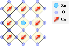
Figure 2: (Color online) Zn-doped CuO₂ plane with natural partitioning in CuO₄ and ZnO₄ clusters.

The substitution of the isovalent Zn²⁺ ion with the nominally completely filled $3d$-shell for Cu²⁺ leaves the oxygen lattice translationally invariant, see Fig. 2. While the electronic levels of Zn doped into a CuO₂ plane have not been determined precisely,Cheng_05 ; Xiang ; Plakida it is generally agreed that the relevant states may occur in a reasonable vicinity of the oxygen level, $\varepsilon_{\rm Zn}-\varepsilon_{p}\simeq 2\!-\!5$eV, and we treat this energy as an adjustable parameter in the following. Thus, the impurity Hamiltonian can be written as

$$\delta{\cal H}_{\rm Zn}=\varepsilon_{\rm Zn}\sum_{\ell\alpha}n^{\rm Zn}_{\ell\alpha}+U_{\rm Zn}\sum_{\ell}n^{\rm Zn}_{\ell\uparrow}n^{\rm Zn}_{\ell\downarrow}$$

$$\phantom{\delta{\cal H}_{\rm Zn}=}-t_{\rm ZnO}\sum_{\langle\ell m\rangle\alpha}\left(a^{\dagger}_{\ell\alpha}p^{\phantom{{\dagger}}}_{m\alpha}+{\rm H.c.}\right)\,,$$ (2)

where Zn sites are labeled with $\ell$, $\varepsilon_{\rm Zn}$ is the energy of the relevant orbital on Zn, $U_{\rm Zn}$ is an effective Hubbard repulsion in that orbital, and $t_{\rm ZnO}$ is the hopping integral between nearest-neighbor Zn and O sites, yet another adjustable parameter. The hole creation/annihilation operators on Zn are $a^{\dagger}_{\ell\alpha}$ and $a^{\phantom{{\dagger}}}_{\ell\alpha}$ and $n^{\rm Zn}_{\ell\alpha}=a^{\dagger}_{\ell\alpha}a^{\phantom{{\dagger}}}_{\ell\alpha}$.

The checkerboard structural motif of the CuO₂ plane in Fig. 2 suggests a natural partitioning of the localized states into symmetric CuO₄ and ZnO₄ clusters, in which each Cu or Zn is surrounded by four oxygens.ZR The advantage of such basic units is in constructing the local states that allow to take into account local hybridization of Cu or Zn and surrounding O states without approximation, while the remaining hybridization between the clusters can be treated perturbatively. In particular, such a cell-perturbation approach does not require Cu-O and Zn-O hopping integrals to be much smaller than the charge-transfer gap $\Delta=\varepsilon_{p}-\varepsilon_{d}$.Jefferson_92 ; Chernyshev_93 ; Chernyshev_94_01 ; Chernyshev_94_02 ; Chernyshev_96

On the other hand, the linear combinations of the oxygen states in CuO₄ (ZnO₄) cluster are not orthogonal to the ones in the nearest-neighbor clusters. The elegant Wannier-orthogonalization procedure, suggested in Ref. ZR, , treats the O-lattice separate from the Cu and Zn, and, via orthogonalizing $p$-operators in the ${\bf k}$-space, leads to the basis of the symmetric-oxygen orbitals

$$\big{\{}p_{m,\alpha}^{x},\;p_{m\alpha}^{y}\big{\}}\rightarrow q_{l,\alpha}(q_{\ell,\alpha})\,,$$ (3)

that are now associated with the same site index as the Cu (Zn) of the CuO₄ (ZnO₄) cluster. The details of this procedure are given in Appendix A.

With that, it is natural to divide the Cu-O (Zn-O) hopping terms in (1) and (2) into the local part, which corresponds to hybridization within one cluster, and into the hopping part, corresponding to the coupling between the states in different clusters. We note, that due to the non-local nature of the Wannier-orthogonalization, the hopping parts now contain terms that go beyond the nearest-neighbor clusters. Thus, the Hamiltonian of (1), written using the orthogonalized basis of O-states (3) is

$${\cal H}^{{\rm loc}}=\sum_{l\alpha}\bigg{\{}\varepsilon_{d}n^{d}_{l\alpha}+\varepsilon_{p}n^{q}_{l\alpha}+\frac{U_{d}}{2}n^{d}_{l\alpha}n^{d}_{l\bar{\alpha}}$$

$$\phantom{{\cal H}^{{\rm loc}}=\sum_{l\alpha}\bigg{\{}}-2\lambda_{0}t_{pd}\left(d^{\dagger}_{l\alpha}q^{\phantom{{\dagger}}}_{l\alpha}+{\rm H.c.}\right)\bigg{\}}$$ (4)

$${\cal H}^{{\rm hop}}=-\sum_{\langle ll^{\prime}\rangle\alpha}2\lambda_{ll^{\prime}}t_{pd}\left(d^{\dagger}_{l\alpha}q^{\phantom{{\dagger}}}_{l^{\prime}\alpha}+{\rm H.c.}\right)\,,$$

where $\lambda_{ll^{\prime}}$ are the Wannier amplitudes given in (24). First, the amplitudes $\lambda_{ll^{\prime}}$ decrease rapidly with distance,Chernyshev_93 $\lambda_{ll^{\prime}}\sim 1/|{\bf r}_{l}-{\bf r}_{l^{\prime}}|^{3}$, so the terms beyond the nearest neighbor in the hopping part of (4) can be neglected. Second, the intra-cluster amplitude $\lambda_{0}=0.9581$ is close to 1, and thus is taking most of the hybridization into account. The nearest-neighbor amplitude $\lambda_{\langle ll^{\prime}\rangle}=0.1401$ leads to the effective hopping parameter between different states that is significantly reduced compared to the bare $t_{pd}$ hopping. This provides a strong justification for the subsequent perturbative expansion in such an effective hopping relative to the effective Hubbard gap, the latter largely defined by the local hybridization.

Applying the same transformation of the O-states (3) to the Hamiltonian of the Zn-cluster (2) we obtain

$$\delta{\cal H}_{\rm Zn}^{{\rm loc}}=\sum_{\ell\alpha}\bigg{\{}\varepsilon_{\rm Zn}n^{\rm Zn}_{\ell\alpha}+\varepsilon_{p}n^{q}_{\ell\alpha}+\frac{U_{\rm Zn}}{2}n^{\rm Zn}_{\ell\alpha}n^{\rm Zn}_{\ell\bar{\alpha}}$$

$$\phantom{\delta{\cal H}_{\rm Zn}^{{\rm loc}}=\sum_{\ell\alpha}\bigg{\{}}-2\lambda_{0}t_{\rm ZnO}\left(a^{\dagger}_{\ell\alpha}q^{\phantom{{\dagger}}}_{\ell\alpha}+{\rm H.c.}\right)\bigg{\}}$$ (5)

$$\delta{\cal H}_{\rm Zn}^{{\rm hop}}=-\sum_{\langle\ell l\rangle\alpha}2\lambda_{\ell l}t_{\rm ZnO}\left(a^{\dagger}_{\ell\alpha}q^{\phantom{{\dagger}}}_{l\alpha}+{\rm H.c.}\right)\,.$$

Note that even if Zn-states are completely neglected in $\delta{\cal H}_{\rm Zn}^{{\rm loc}}$, ZnO₄ cluster still has an unoccupied oxygen statePlakida with the energy $\varepsilon_{p}$, which is higher than the hybridized CuO₄ states of the surrounding clusters, and it permits virtual superexchange processes through it.

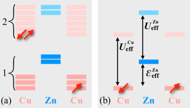
Figure 3: (Color online) (a) A schematic view of the energy levels $E_{i}$ and $\tilde{E}_{i}$ of one- and two-particle sectors in Cu and Zn clusters in Eqs. (6) and (7). (b) The levels of the effective $t-\varepsilon-U$ Hamiltonian that keeps the lowest energy states in each sector.

The next step in the cell-perturbation approach is the diagonalization of ${\cal H}^{{\rm loc}}$ and $\delta{\cal H}^{{\rm loc}}$. Such a diagonalization is performed separately for the states with different number of holes in a cluster. Because the system is close to the half-filling, the most relevant states are the one- and two-hole states, and the states with more holes are higher in energy, see Fig. 3(a). The full set of $d_{l}$, $a_{\ell}$, and $q_{l}$ one- and two-hole states of Cu- and Zn-clusters are listed in Appendix A, (25)-(30), see also Ref. Chernyshev_94_01, .

After the diagonalization of the local parts of the Hamiltonian, the hopping terms are also rewritten in the basis of the new states. Altogether, the three-band model ${\cal H}$ of (4) can be rewritten as a “multi-orbital” Hubbard model with the effective “Cu” eigenstates with local energies $E_{i}$ connected by effective hoppings $F_{ii^{\prime}}^{jj^{\prime}}$:

$${\cal H}=\sum_{li}E_{i}|\psi_{l}^{i}\rangle\langle\psi_{l}^{i}|$$ (6)

$$\phantom{{\cal H}}+\sum_{\langle ll^{\prime}\rangle}\sum_{ii^{\prime}jj^{\prime}}F_{ii^{\prime}}^{jj^{\prime}}\left(|\psi_{l}^{i}\rangle|\psi_{l^{\prime}}^{i^{\prime}}\rangle\langle\psi_{l^{\prime}}^{j^{\prime}}|\langle\psi_{l}^{j}|+{\rm H.c.}\right)\,.$$

Similarly, for $\delta{\cal H}$ of (5)

$$\delta{\cal H}=\sum_{\ell i}\tilde{E}_{i}|\tilde{\psi}_{\ell}^{i}\rangle\langle\tilde{\psi}_{\ell}^{i}|$$ (7)

$$\phantom{\delta{\cal H}}+\sum_{\langle\ell l\rangle}\sum_{ii^{\prime}jj^{\prime}}\tilde{F}^{jj^{\prime}}_{ii^{\prime}}\left(|\tilde{\psi}_{\ell}^{i}\rangle|\psi_{l}^{i^{\prime}}\rangle\langle\psi_{l}^{j^{\prime}}|\langle\tilde{\psi}_{\ell}^{j}|+{\rm H.c.}\right)\,.$$

The hybridized, orthogonal sets of local states are $|\psi_{l}^{i}\rangle$ for CuO₄ and $|\tilde{\psi}_{\ell}^{i}\rangle$ for ZnO₄ clusters, where $l(\ell)$ is the site-index and $i$ is labeling the states. For example, the three one-hole states in Cu cluster in Fig. 3(a) are the “bonding” and “antibonding” mix of Cu and symmetric O states $d_{l}$ and $q_{l}$, Eqs. (21) and (25), and the antisymmetric O-state ($\tilde{q}_{l}$, Eq. (21)). The hopping integrals between adjacent clusters, $F_{ii^{\prime}}^{jj^{\prime}}$ and $\tilde{F}^{jj^{\prime}}_{ii^{\prime}}$, connect initial and final states $i$, $i^{\prime}$ and $j$, $j^{\prime}$.

The Hamiltonian in (6) and (7) is “multi-orbital” because each $n$-particle sector contains more than one state. However, since such states are locally orthogonal and we are interested in the low-energy effective model of (6) and (7), the most important transitions involve the lowest states from each sector, see Fig. 3(a). Importantly, the structure of the lowest states in the single-particle and two-particle sectors of the multi-orbital model is the same as in the one-band Hubbard model, justifying the close correspondence of the three-band and one-band Hubbard models.Jefferson_92 ; Chernyshev_93 ; Chernyshev_94_01 ; Chernyshev_94_02 The lowest one-hole states in Cu- and Zn-cluster are $S=1/2$ doublets, the linear combinations of the oxygen and the Cu(Zn)-orbitals, while the lowest two-hole state is the Zhang-Rice-like singlet, a mix of three different singlets [Cu-Cu, O-O and Cu-O], see (25)-(29).

The new physics is brought in by the possibility of an unoccupied impurity level, the lowest state from the “Zn” single-particle sector, to be lower than the effective Hubbard $U$ on the “Cu” sites. This leads to an effective $t-\varepsilon-U$ model, see Fig. 3(b), which provides surrounding Cu-spins with additional virtual channel for the superexchange processes, connecting spins in the vicinity of impurity. Conversely, if the effective “Zn”-states do not occur below the Hubbard gap (the case of Mg²⁺ due to the lack of available states on it), the impurity can be treated as electronically inert, leading only to dilution, but not to extra interactions. Parameters that control the impurity level are discussed next.

II.2 Parameters and effective impurity level

The realistic values of the three-band model parameters for the CuO₂ plane have a certain degree of variation because none of them is measurable directly and they come as a result of a parametrization of the first-principles calculations. Thus, the Hubbard repulsion on Cu is $U_{d}\!=\!8\!-\!12$eV, the charge-transfer gap $\Delta\!=\!\varepsilon_{p}\!-\!\varepsilon_{d}\!=\!2\!-\!4$eV, and the Cu-O hopping is $t_{pd}\!=\!1\!-\!1.5$eV.Jefferson_92 ; Chernyshev_94_01 ; Chernyshev_94_02 A physical approach to fix them to a particular set of values was suggested in Ref. Chernyshev_94_02, . One can require that the observables, such as the Cu-Cu superexchange or the optical gap, calculated from the model (6) match their observed values. In our case, we fix them to $U_{d}(U_{\rm Zn})\!\gg\!\Delta$, $\Delta\!=\!3$eV, and $t_{pd}\!=\!1.5$eV to yield the experimental value of the superexchange $J\!\simeq\!0.13$eV in the effective low-energy model discussued in Sec. II.C. Among other things, the effective Hubbard gap for the Zhang-Rice-like singlet and the ground state half-filled system is $U_{\rm eff}\!\approx\!3.6$eV.

The parameters of Zn states, such as the bare one-hole level on Zn, $\Delta_{\rm Zn}\!=\!\varepsilon_{\rm Zn}\!-\!\varepsilon_{p}$, and the Zn-O hopping $t_{\rm ZnO}$, are not precisely known.Cheng_05 ; Xiang ; Plakida As is shown in Fig. 4, we vary them substantially to determine the resulting energy of the lowest level in the single-particle sector of the ZnO₄ cluster, $\varepsilon_{\rm eff}^{\rm Zn}$. In Fig. 4(a) we show its dependence on the energy of the bare Zn-level, $\Delta_{\rm Zn}$, for two representative values of $t_{\rm ZnO}$, and in Fig. 4(b) on the the hybridization $t_{\rm ZnO}$ for two representative values of $\Delta_{\rm Zn}$. We also show the effective Hubbard energy $U_{\rm eff}$ to demonstrate the validity of the qualitative level structure in Fig. 3 for a wide range of parameters. Altogether, the electronic levels of Zn and their hybridization with O-states are important in lowering $\varepsilon_{\rm eff}^{\rm Zn}$, and $\varepsilon_{\rm eff}^{\rm Zn}$ is below the Hubbard gap for the realistic parameters of the model.

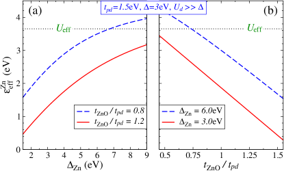
Figure 4: (Color online) (a) Energy of the lowest state from the Zn-cluster single-particle sector, $\varepsilon_{\rm eff}^{\rm Zn}$, vs the energy difference between the bare one-hole levels on Zn and O, $\Delta_{\rm Zn}\!=\!\varepsilon_{\rm Zn}\!-\!\varepsilon_{p}$, for two values of $t_{\rm ZnO}$. (b) $\varepsilon_{\rm eff}^{\rm Zn}$ vs $t_{\rm ZnO}/t_{pd}$ for two representative values of $\Delta_{\rm Zn}$. Parameters of the three-band model are fixed as described in text, $t_{pd}\!=\!1.5$eV, $\Delta\!=\!3$eV, $U_{d}\!\gg\!\Delta$. The resultant Hubbard gap is $U_{\rm eff}\approx 3.6$eV.

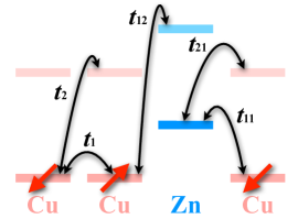
Figure 5: (Color online) Schematic view of various virtual hopping processes between relevant energy levels of the model (6) and (7), see text for notations.

II.3 Projecting to the spin-only model

After establishing the validity of the $t$-$\varepsilon$-$U$-like level structure of Fig. 3 for the realistic parameters of the three-band Hubbard model with Zn impurity, we now turn to the low-energy properties of the model (6) and (7). To derive the low-energy model one needs to consider virtual transitions between different states. As was argued above, since the system is at half-filling, the relevant transitions are between the lowest states from one- and two-hole sector of both Cu- and Zn-cluster states. Altogether, there are five different hopping integrals, as is shown in Fig. 5. For brevity, we switch to $t$’s for the hopping integrals from $F_{ii^{\prime}}^{jj^{\prime}}$ and $\tilde{F}^{jj^{\prime}}_{ii^{\prime}}$ in (6) and (7). For instance, $t_{1}=F_{10}^{01}$ is the hopping of the spin to the neighboring empty site and $t_{2}=F_{11}^{20}$ is creating the Zhang-Rice singlet from the two one-hole sites leaving the other site empty. For the transitions involving Zn-states, $t_{11}$ is between one-hole states on Cu and Zn, while $t_{12}$ and $t_{21}$ are between the one-hole and two-hole states on Cu and Zn. The higher-energy transitions will be neglected as their contributions are small. The explicit expressions for hopping integrals can be obtained by evaluating matrix elements of the Hamiltonian in terms of the original Cu, Zn, and O operators, (4) and (5), between the initial and final states in the basis of the local eigenstates $|\psi_{l}^{i(j)}\rangle$ and $|\tilde{\psi}_{\ell}^{i(j)}\rangle$, see Appendix A for details.

Next, we apply a canonical transformation to this extended $t$-$\varepsilon$-$U$-like model assuming that the hopping integrals are smaller than the effective $U^{\rm Cu}_{\rm eff}$ and $\varepsilon_{\rm eff}^{\rm Zn}$. At half-filling and in the second order, the $t$-$U$ part yields the Heisenberg model with $J=4|t_{2}|^{2}/U_{\rm eff}^{\rm Cu}$ and with the negligible higher-order terms. In the presence of impurity, the same transformation leads to the dilution-only model, in which the four adjacent spin-spin links are cut by the spinless Zn-site. For the sites in the vicinity of impurities, we extend the transformation to the fourth orderTakahashi_77 ; Yoshioka_88 ; Chernyshev_04 in $t/\varepsilon(U)$ to include the -$\varepsilon$- part of the model for the purpose of taking into account the effects of the in-gap impurity state.

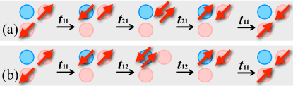
Figure 6: (Color online) Superexchange processes for (a) $\delta J_{1}$, (b) $\delta J_{2}$. See text and Fig. 5 for notations.

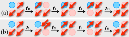
Figure 7: (Color online) Ring-exchanges for (a) $\delta J_{3}$, (b) $\delta J_{4}$.

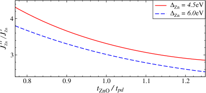
Figure 8: (Color online) The ratio of $J_{\rm Zn}^{\prime\prime}/J_{\rm Zn}^{\prime}$ vs $t_{\rm ZnO}/t_{pd}$ for two representative $\Delta_{\rm Zn}$. Other parameters are as in Fig. 4.

In addition to deriving the low-energy, spin-only model with the parameters that can be traced to the three-band ones, we are also able to analyze individual superexchange processes that contribute to the terms of that model. We find that in the 4^th order there are two types of virtual transitions through the impurity site. First involves three sites, two Cu and one Zn, with the coppers either across the Zn-site or at the right angle, as in Fig. 6. Second type needs three Cu in addition to Zn impurity, arranged in a 4-site plaquette, see Fig. 7. Each of the transition types yields two superexchange channels shown in Figs. 6 and 7. First two, in Fig. 6(a) and (b), are the standard superexchanges, taking four virtual steps instead of the usual two. We denote the corresponding couplings generated by such processes as $\delta J_{1}$ (doubly-occupied state on Cu) and $\delta J_{2}$ (doubly-occupied state on Zn), respectively. The other two processes, in Fig. 7(a) and (b), are the ring exchanges, which we denote as $\delta J_{3}$ (no doubly-occupied state involved) and $\delta J_{4}$ (doubly-occupied state on Cu), respectively. These couplings are given by

$$\delta J_{1}=\displaystyle\frac{4|t_{11}t_{21}|^{2}}{U_{\rm eff}^{\rm Cu}\big{(}\varepsilon_{\rm eff}^{\rm Zn}\big{)}^{2}},\ \ \delta J_{2}=\frac{8|t_{11}t_{12}|^{2}}{\big{(}U_{\rm eff}^{\rm Zn}+2\varepsilon_{\rm eff}^{\rm Zn}\big{)}\big{(}\varepsilon_{\rm eff}^{\rm Zn}\big{)}^{2}},$$

$$\delta J_{3}=-\displaystyle\frac{2|t_{11}t_{1}|^{2}}{\big{(}\varepsilon_{\rm eff}^{\rm Zn}\big{)}^{3}},\ \ \delta J_{4}=-\frac{4|t_{11}t_{1}t_{2}t_{21}|}{U_{\rm eff}^{\rm Cu}\big{(}\varepsilon_{\rm eff}^{\rm Zn}\big{)}^{2}},$$

in terms of the notations of Fig. 5. Assuming that $\varepsilon^{\rm Zn}_{\rm eff}$ is smaller than $U_{\rm eff}$ according to the discussion of Sec. II.B, the magnitudes of $\delta J_{i}$’s should substantially exceed the conventional fourth-order terms of order $t_{\rm eff}^{4}/U_{\rm eff}^{3}$, which we neglect. Another important distinction of the couplings in (II.3), is that they occur due to impurities and thus must have a direct relation to the doping-dependent effects. Altogether, the considered processes combine into the next-nearest- and next-next-nearest-neighbor frustrating interactions around Zn-impurity, see Fig. 1(c),

$$J^{\prime}_{\rm Zn}=\delta J_{1}+\delta J_{2}+\delta J_{3}+\delta J_{4},$$ (9)

$$J^{\prime\prime}_{\rm Zn}=\delta J_{1}+\delta J_{2}.$$

It is clear that only superexchange-type processes of Fig. 6 can contribute to the next-next-nearest-neighbor couplings across the impurity $J^{\prime\prime}_{\rm Zn}$, while the ring-exchanges of Fig. 7 are also at play for $J^{\prime}_{\rm Zn}$. Importantly, the latter terms have a ferromagnetic sign, reducing the value of $J^{\prime}_{\rm Zn}$ compared to $J^{\prime\prime}_{\rm Zn}$. Thus, counterintuitively, the longer-ranged $J^{\prime\prime}_{\rm Zn}$ should be greater than $J^{\prime}_{\rm Zn}$. This feature is made explicit in our Fig. 8, which shows that the ratio of $J^{\prime\prime}_{\rm Zn}/J^{\prime}_{\rm Zn}$ varies from about 4 to 2 for a representative range of the electronic parameters of Zn with the other three-band model parameters as in Fig. 4.

As is shown in Fig. 1(c), each impurity generates four $J^{\prime}_{\rm Zn}$ and two $J^{\prime\prime}_{\rm Zn}$. Thus, the total frustrating effect per Zn-impurity is $J_{\rm Zn}^{tot}=4J^{\prime}_{\rm Zn}+2J^{\prime\prime}_{\rm Zn}$. We show the dependence of $J_{\rm Zn}^{tot}$ on $\Delta_{\rm Zn}$ and $t_{\rm ZnO}$ in Fig. 9 with the same set of three-band parameters as in Sec. II.B and in Fig. 4. The shaded area in the graphs shows the range of $J_{\rm Zn}^{tot}$ needed to explain experimentally observed reduction of the staggered magnetization $M(x)/M(0)$, according to the $T$-matrix discussion of Sec. III. Clearly, the uncertainty in the electronic parameters of Zn-orbitals does not allow us to provide significant restrictions on the value of $J_{\rm Zn}^{tot}$. However, the values needed for $M(x)/M(0)$ doping dependence outline the minimal requirements on such three-band model parameters. In particular, the coupling of Zn and O orbitals should not be much weaker than that of Cu and O, while the position of the level on Zn is much less restricted. Overall, the realistic requirements on Zn electronic degrees of freedom leave a wide range of $J_{\rm Zn}^{tot}$ and they support the validity of our proposed impurity-induced frustration mechanism.

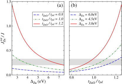
Figure 9: (Color online) The total frustration effect per Zn impurity $J_{\rm Zn}^{tot}=4J^{\prime}_{\rm Zn}+2J^{\prime\prime}_{\rm Zn}$ (a) vs $\Delta_{\rm Zn}$ for several representative values of $t_{\rm ZnO}$ and (b) vs $t_{\rm ZnO}/t_{pd}$ for several values of $\Delta_{\rm Zn}$, respectively. Three-band parameters are $t_{pd}\!=\!1.5$eV, $\Delta\!=\!3$eV, $U_{d}\!\gg\!\Delta$ as before. The shaded area is the range of $J_{\rm Zn}^{tot}$ needed to explain experimental reduction of the staggered magnetization $M(x)/M(0)$, see Sec. III.

Finally, the effective low-energy, spin-only model for La₂Cu_1-xZn_xO₄ can be divided into two parts

$${\cal H}=J\sum_{\langle ll^{\prime}\rangle}\mathbf{S}_{l}\cdot\mathbf{S}_{l^{\prime}}+J_{\rm Zn}^{\prime}\sum_{\langle ll^{\prime}\rangle^{\prime}_{\ell}}\mathbf{S}_{l}\cdot\mathbf{S}_{l^{\prime}}+J_{\rm Zn}^{\prime\prime}\sum_{\langle ll^{\prime}\rangle^{\prime\prime}_{\ell}}\mathbf{S}_{l}\cdot\mathbf{S}_{l^{\prime}},\ \ \$$ (10)

the dilution-only model (first term), and the impurity-induced frustrating terms, with $\langle ll^{\prime}\rangle^{\prime}_{\ell}$ and $\langle ll^{\prime}\rangle^{\prime\prime}_{\ell}$ denoting next- and next-next-nearest-neighbor bonds that are also nearest-neighbors of the impurity site $\ell$, see Fig. 1(c). The summations are carried over the Cu sites only.

We propose that the dilution-frustration model (10) provides a proper description of Zn-doped CuO₂ planes and discuss its properties next.

III On-site magnetization in the low-energy model

With the structure of the low-energy spin-only model for CuO₂ plane diluted by Zn impurities given in (10), we investigate in detail the impact of impurities on the order parameter, the average on-site magnetization $M$. We use the linear spin-wave approximation to the problem of single impurity in the model (10) and apply an analytical $T$-matrix approach to it, which is based on summing up exactly infinite diagrammatic series for the impurity scattering amplitudes. Then we approximate the problem of finite concentration of impurities as a linear superposition of scattering effects of individual random impurities, which amounts to an “effective medium” approach via disorder averaging. This step restores translational invariance for magnons but modifies their dispersion and provides them with damping through the impurity scattering self-energies. The averaging also takes into account the increase of the population of magnons around impurities, i.e., for the extra fluctuations of spins that reduce the value of the ordered moment. The latter effect is calculated from the renormalized magnon Green’s function as a function of impurity concentration $x$.Chernyshev_01 ; Chernyshev_02

We note that the order parameter is normalized by the number of magnetic ions: $M(x)=\sum_{i}|S_{i}^{z}|/N_{m}$, where $N_{m}=N-N_{imp}$ is the number of magnetic sites (Cu²⁺) and $N$ is the total number of sites. The reason for that is twofold. First, the experimental data on $M(x)$ from such techniques as NMR[NQR] and neutron scattering are naturally normalized this way. Second, such a normalization also separates the classical effect of dilution from the purely quantum-mechanical suppression of the order parameter. For instance, $M(x)$ defined this way is close to a constant for the classical (Ising) antiferromagnet on a square lattice, as is shown in Fig. 10(a), because this quantity is equivalent to a probability for a spin to belong to an infinite cluster, which is very close to 1 below the percolation threshold, $x_{p}\approx 41\%$.

In this Section, we first demonstrate the discrepancy of the previous theoretical works based on the dilution-only model with experimental data and then proceed with the calculations within the dilution-frustration model of Eq. (10). Comparison with experimental data provides a confirmation of the selfconsistency of our consideration in two respects. First, it allows us to verify whether the impurity-induced frustration is at all a reasonable mechanism of producing extra suppression of the order parameter. Second, we are able to compare the range of parameters $J^{\prime}_{\rm Zn}$ and $J^{\prime\prime}_{\rm Zn}$ that are necessary to explain the experimental data for $M(x)$ with the range permitted by the three-band Hubbard mapping of Sec. II.

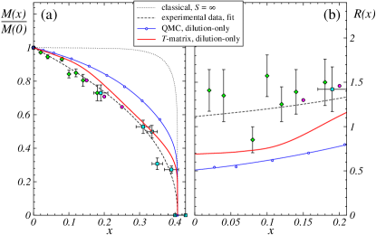
Figure 10: (Color online) (a) The on-site magnetic moment $M(x)$ per magnetic site (Cu²⁺), normalized to the undoped value $M(0)$ vs Zn doping $x$. Green diamonds and magenta circles are the NQR data,Corti_95 ; Carretta_97 cyan squares are the neutron scattering data,Greven_03 and the dashed line is their best fit. The dotted line is the classical (Ising) result. Upper solid line (blue online) is the best fit of the QMC results (blue circles)Sandvik02a and the lower solid line (red online) is the $T$-matrix calculation results,Chernyshev_02 both for the dilution-only model. (b) The slope function $R(x)$ of normalized staggered magnetization (see text) vs $x$. Symbols and lines are the same as in (a).

III.1 Discrepancy with experiments

Our Fig. 10(a) shows a comparison of the results for the averaged on-site magnetic moment (staggered magnetization) $M(x)$, normalized to its value in the undoped system $M(0)$. The experimental data include the NQRCorti_95 ; Carretta_97 and the neutron scattering data,Greven_03 with the dashed line being their best fit. Both set of theoretical results, from the QMCSandvik02a and the $T$-matrixChernyshev_02 calculations, are for $T=0$ dilution-only model, i.e., neglecting frustrating effects of impurities proposed in this work. First observation is that the unbiased QMC data agree very closely with the $T$-matrix results up to $x\simeq 15\%$, thus supporting the validity of the latter in the low-doping regime.Chernyshev_02 ; Sandvik02a At higher doping, single-impurity $T$-matrix tends to overestimate the effect of impurities on the order parameter. Note that the $T$-matrix results in Fig. 10(a) are multiplied by the classical probability (dotted line). This does not affect the data for $x<35\%$ but makes a comparison consistent near the percolation threshold $x_{p}$.

However, there are substantial discrepancies between theoretical and experimental results. In Fig. 10(a) the experimental data are always below the theoretical curves for the dilution-only model. The difference is much more apparent in the slope function, defined as

$$R(x)=\frac{1}{x}\bigg{(}1-\frac{M(x)}{M(0)}\bigg{)}\,,$$ (11)

and displayed in Fig. 10(b). The quantity $R(x)$ has a transparent physical meaning at $x\rightarrow 0$: it shows a reduction of the order parameter $M$ per impurity due to enhanced quantum fluctuations in the impurity’s neighborhood, the quantity that should be captured properly by the $T$-matrix approach. Fig. 10(b) shows a large discrepancy of the experimental slope, $R^{\rm exp}(0)\approx 1.1$, with both the QMC, $R^{\rm QMC}(0)\approx 0.5$, a factor of approximately 2, and the $T$-matrix, $R^{T}(0)\approx 0.7$, a factor of about 1.6. This gives a clear indication that the dilution-only theory significantly underestimates the impact of the individual impurities on the quantum spin background. Thus, the dilution-only model is not enough to describe La₂Cu_1-xZn_xO₄.

III.2 Qualitative $J_{1}^{\rm eff}$-$J_{2}^{\rm eff}$-$J_{3}^{\rm eff}$ mean-field consideration of the dilution-frustration model

We would like to argue that the longer-ranged spin interactions in the undoped system are unlikely to provide a resolution to the observed discrepancy in $M(x)$. On the other hand, the dilution-frustration model of Eq. (10) can be approximated on a mean-field level as an effective model with further exchanges that are proportional to doping. Such a mean-field consideration offers a simple way of checking the viability of this model in explaining the discrepancy.

One of the natural ideas to explain the disagreement is by including the longer-range interactions, such as $J_{2}$, $J_{3}$, etc., and ring-exchange, in the low-energy spin-only model for the undoped CuO₂ plane. Such terms are generally present in any realistic low-energy spin models of Mott insulators and formally come as a result of the higher-order expansion of the Hubbard-like models.Chernyshev_04 Although for the cupratesDelannoy_09 such terms are of the order of 10% of the nearest-neighbor $J$, they do lead to a reductionTremblay_09 of $M$. Qualitatively, assuming the presence of $J_{2}$ term in the spin-model and using an expansion of $M$ in the dilution fraction $x$ and in $J_{2}$, one can obtain on the mean-field level at small $x$ and $J_{2}$:

$$R(J_{2})\approx R(0)\left(1+A\frac{J_{2}}{J}\right),$$ (12)

where the coefficient $A\lesssim 1$ follows from the consideration of the $J_{1}$-$J_{2}$ modelSchulz_96 and $R(0)$ is the theoretical slope of the dilution-only model in Fig. 12(b). Thus, unless $J_{2}$ is of the same order as $J$, one can not expect a large correction to the slope of $M(x)/M(0)$ from the presence of further-neighbor terms in the low-energy model.

In addition, since these terms suppress the order already in the undoped system, this mechanism is unlikely to enhance fluctuations specifically due to dilution. Put another way, dilution of the models with extended interactions breaks frustrated bonds alongside the nearest-neighbor ones and may even induce more robust order around impurities. A recent detailed studyDelannoy_09 has shown that while extended interactions such as $J_{2}$ and cyclic terms do lead to an overall lower absolute values of the on-site magnetization in the impurity-doped Hubbard model of La₂Cu_1-xZn_xO₄, they do not significantly change the theoretical $M(x)/M(0)$ dependence and are not able to explain the large experimental slope $R(x)$ in Fig. 12(b).

On the other hand, the dilution-frustration model of Eq. (10) offers an alternative: while the undoped system can be considered as having no further-neighbor frustrating terms in its low-energy model, such terms are introduced by the dopants. We thus propose an “effective medium”, mean-field $J_{1}^{\rm eff}$-$J_{2}^{\rm eff}$-$J_{3}^{\rm eff}$ model, in which effective interactions depend on the doping concentration $x$, as a simplified version of the dilution-frustration model (10) that allows for a straightforward calculation of $M(x)$ without the complications of the $T$-matrix or QMC numerical approaches. While approximate, this method gives an intuitive picture of the proposed mechanism and allows us to estimate whether it can be a viable source of enhancing quantum fluctuations due to doping.

In a sense, the mean-field approximation “spreads” the frustration provided by impurities evenly over the whole system. The strength of the effective couplings is related to the exchanges in (10) by counting bonds: nearest-neighbor interaction $J_{1}^{\rm eff}=J(1-2x)$, next-nearest-neighbor interaction $J_{2}^{\rm eff}=2xJ_{\rm Zn}^{\prime}$, and next-next-nearest-neighbor interaction $J_{3}^{\rm eff}=xJ_{\rm Zn}^{\prime\prime}$. Since we are interested in $x\ll 1$ limit, the derivation of $M$ amounts to on expansion of the spin-wave correction to the order parameter within the $J_{1}^{\rm eff}$-$J_{2}^{\rm eff}$-$J_{3}^{\rm eff}$ model to the first power in $J_{2}^{\rm eff}/J$ and $J_{3}^{\rm eff}/J$. Using the approach of Ref. Schulz_96, we obtain the moment reduction as

$$\frac{M(x)}{M(0)}\simeq 1-\frac{C_{2}}{M(0)}\left(\frac{J_{2}^{\rm eff}}{J}\right)-\frac{C_{3}}{M(0)}\left(\frac{J_{3}^{\rm eff}}{J}\right)\,,$$ (13)

where $C_{2(3)}=\sum_{\bf k}\eta_{2(3),{\bf k}}\gamma_{\bf k}^{2}/2\omega^{3}_{\bf k}$, with $\omega_{\bf k}=\sqrt{1-\gamma_{\bf k}^{2}}$, $\gamma_{\bf k}=(\cos k_{x}+\cos k_{y})/2$, $\eta_{2,{\bf k}}=(1-\cos k_{x}\cos k_{y})$, $\eta_{3,{\bf k}}=(2-\cos^{2}k_{x}-\cos^{2}k_{y})$, and $M(0)=0.3034$ is the ordered moment of the $S=1/2$, square-lattice nearest-neighbor Heisenberg antiferromagnet in the spin-wave approximation. Interestingly, since the $C_{2}=0.2909$ and $C_{3}=0.5205$, the suppression of the order by $J_{3}^{\rm eff}$ is almost two times as effective as by $J_{2}^{\rm eff}$ of the same value. Setting the change of the slope, which is needed for the dilution-only result $R^{T}(0)\approx 0.7$ to achieve the agreement with experimental $R^{\rm exp}(0)\approx 1.1$, and using the relation of $J_{2}^{\rm eff}$ and $J_{3}^{\rm eff}$ to $J_{\rm Zn}^{\prime}$ and $J_{\rm Zn}^{\prime\prime}$ we can determine the range of $J_{\rm Zn}^{tot}=2J_{\rm Zn}^{\prime\prime}+4J_{\rm Zn}^{\prime}$ necessary for that. Assuming $J_{2}^{\rm eff}=J_{3}^{\rm eff}$ corresponds to the choice $J_{\rm Zn}^{\prime\prime}=2J_{\rm Zn}^{\prime}$, which is a reasonable ratio according to the three-band model consideration, see Fig. 8. Using (13), the required total frustrating effect due to each impurity is $J_{\rm Zn}^{tot}\simeq 0.6J$, which is well within the range of the estimates from the three-band model mapping, see Fig. 9.

Altogether, this consideration shows that the dilution-frustration model is indeed a viable candidate for explaining the discrepancy with the experimental data.

III.3 $T$-matrix for the dilution-frustration model

A more rigorous, albeit more technically involved method of dealing with the dilution-frustration model (10) is the $T$-matrix approach. Its advantage is in taking into account all multiple-scattering magnon processes, by which it solves the single-impurity problem exactly within the $1/S$ spin-wave approximation. Since we are interested in identifying a mechanism of the order parameter suppression in the low-doping regime, such an approach should be able to provide if not the ultimate, but at least a quantitatively correct result.

The $T$-matrix method has been used in the study of the dilution-only model in the 2D square-lattice antiferromagnet.Bulut ; kampf ; Mahan ; Wan ; NN ; Sandvik ; KK_imp ; Yasuda ; Chernyshev_01 ; Chernyshev_02 Here we outline some of the basic steps needed to calculate staggered magnetization in the dilution-frustration model (10) and provide necessary details in Appendix B.

Staggered magnetization at $T=0$ in the presence of impurities can be written asChernyshev_02

$$M(x)=M(0)-\sum_{\bf k}\frac{1}{\omega_{\bf k}}\left(\langle\alpha^{\dagger}_{\bf k}\alpha^{\phantom{{\dagger}}}_{\bf k}\rangle-\gamma_{\bf k}\langle\alpha^{\dagger}_{\bf k}\alpha^{\dagger}_{\bf-k}\rangle\right)\,,\ \ \$$ (14)

where $M(0)=S-\Delta\simeq 0.3034$ is the staggered magnetization of the $S=1/2$, square-lattice, nearest-neighbor Heisenberg antiferromagnet at zero-doping, which is already reduced by quantum fluctuations ($\Delta$) of the antiferromagnetic ground state, and $\omega_{\bf k}=\sqrt{1-\gamma_{\bf k}^{2}}$ as before. Quantum fluctuations due to impurities further reduce $M(x)$ by non-zero magnon expectation values $\langle\alpha^{\dagger}_{\bf k}\alpha^{\phantom{{\dagger}}}_{\bf k}\rangle$ and $\langle\alpha^{\dagger}_{\bf k}\alpha^{\dagger}_{\bf-k}\rangle$. These can be expressed through the magnon Green’s function,Chernyshev_02 leading to

$$\frac{M(x)}{M(0)} = 1-\frac{1}{M(0)}\sum_{\bf k}\int_{-\infty}^{0}\frac{d\omega}{\pi\omega_{\bf k}}\Big{(}{\rm Im}G_{\bf k}^{11}(\omega)$$ (15)

$$\phantom{-\frac{1}{M(0)}\sum_{\bf k}\int_{-\infty}^{0}\frac{d\omega}{\pi\omega_{\bf k}}}-\gamma_{\bf k}{\rm Im}G_{\bf k}^{12}(\omega)\Big{)}\,,\ \$$

where $G_{\bf k}^{11}$ and $G_{\bf k}^{12}$ are the diagonal and the off-diagonal component of the $2\times 2$ matrix Green’s function, respectively, see Eq. (34) for the corresponding Dyson-Belyaev expression of them via the magnon self-energies. We note that ${\rm Im}G_{\bf k}^{11}(\omega)>0$ for $\omega<0$. Magnon self-energy in this approach comes as a result of averaging over random impurity distribution, which relates it to the forward-scattering (${\bf k}^{\prime}={\bf k}$) elements of the $T$-matrix

$$\mathbf{\hat{\Sigma}}_{\bf k}(\omega)=x\sum_{\mu,I}\delta_{{\bf k},{\bf k}^{\prime}}\mathbf{\hat{T}}^{I\mu}_{{\bf k},{\bf k}^{\prime}}(\omega)\,.$$ (16)

Here the sum includes the contributions from impurities in both sublattices ($I=A$, $B$) and from each of the non-zero $\mu=s$-, $p$-, and $d$-wave components of the $T$-matrix for the vacancy in the nearest-neighbor square lattice. Clearly, the self-energies are also proportional to the impurity concentration $x$.

The individual components of the $T$-matrix (38) obey linear integral equations for the multiple-scattering in each partial wave. Such equations contain separable scattering potentials, which reduce integral equations to simple algebraic ones and allow for solutions in a separable form. That is, each partial wave $T$-matrix $\mathbf{\hat{T}}^{I\mu}_{{\bf k},{\bf k}^{\prime}}(\omega)$ is given by the product of the ${\bf k}$- and ${\bf k}^{\prime}$-dependent scattering potential components with the corresponding $\omega$-dependent resolvents,Chernyshev_02 see Eqs. (38), (39), (40), and (41) in Appendix B.

The dilution-frustration model (10) contains extra frustrating antiferromagnetic terms compared to the dilution-only model, $J_{\rm Zn}^{\prime}$ and $J_{\rm Zn}^{\prime\prime}$, that couple spins around impurities. We find that because these extra terms connect spins that belong to the same antifferomagnetic sublattice of the host, additional scattering provided by them is orthogonal to the $s$-wave due to a cancellation between $S^{z}S^{z}$ and $S^{+}S^{-}$ contributions. For the same reason, the next-next-nearest-neighbor interaction $J_{\rm Zn}^{\prime\prime}$ also does not modify the $d$-wave component of the scattering potential and contributes only to the $p$-wave, while the next-nearest-neighbor $J_{\rm Zn}^{\prime}$ interaction affects both the $d$-wave and the $p$-wave scattering, see (39) and (B).

While the $x$-dependence of Eq. (15) obviously extends beyond linear, it is the linear term which is of primary importance as it is defining the initial slope of the normalized magnetization, $R(0)$ in (11). It is also the term that is expected to be treated properly by the $T$-matrix approach. Thus, one may want to simplify the general expression (15) and obtain an expression which is explicitly linear in $x$. Having in mind that all magnon self-energies in (16) are $\propto x$, we use the Green’s function expansion in $\hat{\Sigma}$, see (35), to obtain

$$\frac{M(x)}{M(0)}\simeq 1-xR(0)=1-\frac{1}{M(0)}\sum_{\bf k}\Bigg{\{}\frac{-\gamma_{\bf k}{\rm Re}\Sigma_{\bf k}^{12}(\omega_{\bf k})}{2\omega_{\bf k}^{2}}$$

$$\phantom{\frac{M(x)}{M(0)}}+\int_{-\infty}^{0}\frac{d\omega}{\pi\omega_{\bf k}}\left[\frac{{\rm Im}\Sigma_{\bf k}^{11}(\omega)}{\big{(}\omega-\omega_{\bf k}\big{)}^{2}}+\frac{\gamma_{\bf k}{\rm Im}\Sigma_{\bf k}^{12}(\omega)}{\big{(}\omega^{2}-\omega_{\bf k}^{2}\big{)}}\right]\Bigg{\}},$$ (17)

where we note again that ${\rm Im}\Sigma_{\bf k}^{11}(\omega)>0$ for $\omega<0$. With this, we can study the effect of impurity-induced frustration on the order parameter by calculating integrals in (17) and (15) for different values of $J_{\rm Zn}^{\prime}$ and $J_{\rm Zn}^{\prime\prime}$.

First, in agreement with the qualitative consideration provided by the mean-field $J_{1}^{\rm eff}$-$J_{2}^{\rm eff}$-$J_{3}^{\rm eff}$ model in Sec. III.B, we find that the next-next-nearest neighbor $J^{\prime\prime}_{\rm Zn}$ bond suppresses the order about as effectively as two next-nearest $J^{\prime}_{\rm Zn}$ bonds of the same strength. As was discussed in our previous work,Liu_09 the same result has also been obtained by the QMC calculations, confirming again a good qualitative and quantitative accord between the analytical $T$-matrix approach and an unbiased numerical method. Since the three-band model calculations of Sec. II also suggest that the $J^{\prime\prime}_{\rm Zn}$-term is systematically larger than the $J^{\prime}_{\rm Zn}$-term, these findings make the $J^{\prime\prime}_{\rm Zn}$ interaction particularly important.

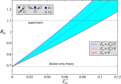
Figure 11: (Color online) $R(0)$ from (17) vs $J_{\rm Zn}^{\prime\prime}$ (in units of $J$). The red solid, magenta dotted-dashed, and blue dashed lines are for $J^{\prime}_{\rm Zn}/J^{\prime\prime}_{\rm Zn}=0$, $1/4$ and $1/2$, respectively. Colored area highlights the range of $J_{\rm Zn}^{\prime\prime}$. The experimental value $R^{exp}(0)$ and the dilution-only $T$-matrix resultChernyshev_02 of $R^{T}(0)$ are shown by the dotted horizontal lines.

We study the rate of suppression of the order parameter $R(0)$ in (17) for several representative ratios between $J^{\prime}_{\rm Zn}$ and $J^{\prime\prime}_{\rm Zn}$ as a function of one of them. Our Fig. 11 shows $R(0)$ vs $J^{\prime\prime}_{\rm Zn}$ for three choices of $J^{\prime}_{\rm Zn}/J^{\prime\prime}_{\rm Zn}=0$, $1/4$ and $1/2$. The dilution-only $T$-matrix resultChernyshev_02 of $R^{T}(0)\approx 0.69$ and the “target” experimental value $R^{exp}(0)\approx 1.1$ are shown by the dotted horizontal lines. We find the effect of frustrating interactions to be about two times stronger than in the mean-field $J_{1}^{\rm eff}$-$J_{2}^{\rm eff}$-$J_{3}^{\rm eff}$ consideration of Sec. III.B, implying that the averaged mean-field treatment underestimates the effect of the order suppression due to frustration by local defects. This result also means that the necessary frustration is smaller than the one estimated from the $J_{1}^{\rm eff}$-$J_{2}^{\rm eff}$-$J_{3}^{\rm eff}$ model.

One can see that the experimental value of $R(0)$ in Zn-doped La₂CuO₄ is met by the $T$-matrix results of the dilution-frustration model at $J^{\prime\prime}_{\rm Zn}\approx 0.07J$ if the ratio of $J^{\prime}_{\rm Zn}/J^{\prime\prime}_{\rm Zn}$ is fixed to $1/2$ and at $J^{\prime\prime}_{\rm Zn}\approx 0.08J$ for $J^{\prime}_{\rm Zn}/J^{\prime\prime}_{\rm Zn}=1/4$, the window of variation of $J^{\prime}_{\rm Zn}/J^{\prime\prime}_{\rm Zn}$ suggested by the three-band model consideration in Fig. 9 of Sec. II. These values translate into the total frustrating effect of impurity $J_{\rm Zn}^{tot}\approx 0.28J$ and $J_{\rm Zn}^{tot}\approx 0.24J$, respectively, which are well within the window suggested by the three-band model calculations. The somewhat wider range is highlighted by the gray shaded area in Fig. 9(a) and (b).

In our previous work,Liu_09 QMC results seem to suggest a higher value $J_{\rm Zn}^{tot}\!\gtrsim\!0.4J$, still a modest amount of frustration, well within the range permitted by the three-band model. An example of the QMC results for $R^{QMC}(0)$ for the choice of parameters $J^{\prime\prime}_{\rm Zn}\!=\!2J^{\prime}_{\rm Zn}\!=\!0.1J$ is shown in Fig. 12(b) by the blue diamond on the vertical axis. However, the QMC calculations may be affected by the frustrating nature of the impurity-induced interactions, which is associated with the infamous sign problem. This is also restricting the use of the QMC for the dilution-frustration model to the single-impurity problem. In addition, the QMC results for $R^{QMC}(0)$ are obtained from the finite-size scaling that may overestimate $J_{\rm Zn}^{tot}$. Thus, using the data only from the largest clusters,Liu_09 extrapolation for the $J^{\prime\prime}_{Zn}\!=\!2J^{\prime}_{Zn}\!=\!0.1J$ data set gives $R^{QMC}(0)\!\approx\!1.0$, much closer to the experimental value. Thus, the QMC result also demonstrates that the impurity-induced frustrations affect the staggered magnetization significantly and bring the slope much closer to experimental data.

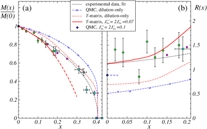
Figure 12: (Color online) Same as Fig. 10 with the lines used for the fit of the QMC data and for the $T$-matrix results of the dilution-only case switched to the dashed lines for clarity. The red solid line (and its long-dashed line tail) is the $T$-matrix results (15) for the dilution-frustration model with $J_{\rm Zn}^{\prime\prime}=2J_{\rm Zn}^{\prime}=0.07J$. In (b) the blue diamond with the dashed line is the QMC result for $J_{\rm Zn}^{\prime\prime}=2J_{\rm Zn}^{\prime}=0.1J$ from Ref. Liu_09, .

Using Eq. (15) we calculate the normalized staggered magnetization and the slope (11) for the dilution-frustration model with $J_{\rm Zn}^{\prime\prime}=2J_{\rm Zn}^{\prime}=0.07J$ as a function of $x$, with the results shown in Fig. 12(a) and (b) by the solid lines. The comparison is provided with the experimental data and the theoretical $T$-matrix and QMC calculations for the dilution-only model from Fig. 10. With the frustrating parameters chosen to match the initial slope of the experimental best fit, obviously, $M(x)/M(0)$ in the dilution-frustration model agrees much better with experiments. At higher values of $x\gtrsim 15\%$, the $T$-matrix overestimates the effect of impurities on $M(x)$ as it neglects the multiple-impurity scattering effects, similarly to the dilution-only case.

Altogether, all of the evidences indicate that the dilution-frustration model describes La₂Cu_1-xZn_xO₄ better than the dilution-only model and that the effective frustrating interactions via available electronic states of the impurity should be taken into account when studying doped Mott- and charge-transfer insulators.

III.4 Further developments

Based on the analysis of the Néel temperature doping dependence within the classical Heisenberg model, an alternative suggestion has been put forward for additional interactions introduced by dopants, such as Mg and Zn: lattice distortions in the vicinity of the impurity site change the strength of $J$ bonds.Oguchi The impact of this mechanism on $M(x)$ and its possible viability as an alternative to our proposal has been investigated using the QMC analysis in Ref. LiuKao10, . It was found that changing the strength of the eight Cu-Cu bonds in the immediate vicinity of Zn site by as much as 15% ($\equiv\delta\widetilde{J}_{tot}=1.2J$) changes the slope of $M(x)/M(0)$ by at most a few percent. Such a weak effect rules out the lattice-distortion mechanism as a viable alternative to our theory.

One of the natural consequences of our idea is that different isovalent impurities, such as Zn²⁺ and Mg²⁺, should induce different amount of quantum fluctuations around them due to differences in their electronic levels available to generate frustrating interactions, and thus lead to a different rate of suppression of the order parameter. Specifically, Mg²⁺ should have no levels in any reasonable proximity to the chemical potential, as opposed to Zn²⁺, and thus should not lead to any substantial frustration, suggesting that the Mg-doped La₂CuO₄ must be described much better by a simple dilution-only model. This scenario has been investigated recently by the $\mu$SR experiments in Zn- and Mg-doped La₂CuO₄ at low doping.Carretta_11 The crucial finding of this work is that the spin stiffness, determined from the Néel temperature, shows a stronger suppression rate in the case of Zn-doping, in agreement with the expectations from our theory. Although in additional to quantum contributions the slope of $T_{N}(x)/T_{N}(0)\approx 1-\alpha x$ contains significant classical terms as well as logarithmic contributions from the three-dimensional interplane couplings,Chernyshev_02 ; Oguchi the difference in such slopes found in Ref. Carretta_11, is significant: $\alpha_{\rm Mg}\approx 2.7$ vs $\alpha_{\rm Zn}\approx 3.5$. These values are consistent with the difference expected between the dilution-only modelChernyshev_02 and the dilution-frustration model with the parameters discussed in Sec. III.C.

IV conclusions

In this work, we have provided a detailed derivation of the low-energy, spin-only model of the Zn-doped La₂CuO₄ starting from the realistic site-diluted three-band Hubbard model. We have followed with an equally detailed analysis of the order parameter in this low-energy model. We have elaborated on the proposal of our previous work that the impurities in strongly correlated systems may induce significant longer-range frustrating interactions among the spins, which are absent or negligible in the corresponding undoped system, due to hybridized electronic states of the impurity at the scale less than the Hubbard-$U$. Such impurity-induced frustrating interactions are shown to significantly enhance local quantum fluctuations compared to the dilution-only model. In particular, the dilution-frustration model demonstrates stronger suppression of the order and, for a choice of parameters appropriate for Zn-doped La₂CuO₄, it resolves discrepancies between experiments and earlier theories. Recently, our theory has received further experimental confirmation from the $\mu$SR studies of spin stiffness in Zn and Mg doped La₂CuO₄.

Although our work considers a particular case of diluted La₂CuO₄, this study has far-reaching consequences for other diluted antiferromagnets and doped Mott and charge-transfer insulators.Zaliznyak One of the intriguing consequences of the proposed mechanism is the change of the character of the percolation transition due to frustrating interactions across the impurities. The impurity doping of one-dimensional spin systems such as spin chains and ladders should introduce weaker links between their parts instead of breaking them into independent pieces. Experiments in diluted frustrated spin systems is yet another area, such as recently studied diluted $J_{1}$-$J_{2}$ system,Carretta_05 ; Carretta_12 which should also be affected by the same mechanism. Another perspective is offered by an extension of the proposed mechanism of the impurity-induced frustrating interactions to the case of the doping away from half-filling where it may be responsible for the pair-breaking mechanism in the doped CuO₂ planes.

Appendix A Details of the three-band model consideration

A.1 Wannier orthogonalization of oxygen orbitals

The hopping terms in the three-band model (1) and (2) couple the Cu and Zn states with the symmetric combination of O-states, i.e.,

$${\cal H}_{pd}=-t_{pd}\sum_{l\alpha}\left(d^{\dagger}_{l\alpha}P^{\phantom{\dagger}}_{l\alpha}+{\rm H.c.}\right)\,,$$ (18)

with

$$P^{\phantom{\dagger}}_{l\alpha}=\left(p^{x}_{l+\frac{{\bf x}}{2}}+p^{x}_{l-\frac{{\bf x}}{2}}+p^{y}_{l+\frac{{\bf y}}{2}}+p^{y}_{l-\frac{{\bf y}}{2}}\right)_{\alpha}\,,$$ (19)

where ${\bf x}$ and ${\bf y}$ are the vectors in the $x$ and $y$ direction of length $a_{0}=1$, the CuO₂ lattice spacing. The problem is that the operators $P_{l\alpha}$ do not obey proper anticommutation relations with the ones on the nearest-neighbor CuO₄(ZnO₄) clusters, because one of the four $p$-operators in (19) belongs to both clusters. The Wannier-orthogonalization procedure is performed in the ${\bf k}$-space.ZR ; Chernyshev_94_01 Since the O-lattice is fully periodic even for the CuO₂ plane doped with Zn, the Fourier transform of the oxygen-hole operators $p_{m}^{x(y)}$ can be written as

$$p^{x(y)}_{m\alpha}=\frac{1}{\sqrt{N}}\sum_{\bf k}e^{-i{\bf k}\cdot\left({\bf r}_{l}\pm\frac{{\bf x}}{2}\left(\frac{{\bf y}}{2}\right)\right)}\,p^{x(y)}_{{\bf k},\alpha},$$ (20)

where the sum is over the Brillouin zone and $N$ is the number of unit cells.

Motivated by (19) and using (20), one can introduce the orthogonalized symmetric and antisymmetric oxygen operators in momentum space as

$$q_{{\bf k},\alpha}=\lambda_{\bf k}^{-1}\bigg{[}\cos\left(\frac{k_{y}}{2}\right)p^{y}_{{\bf k},\alpha}+\cos\left(\frac{k_{x}}{2}\right)p^{x}_{{\bf k},\alpha}\bigg{]},$$ (21)

$$\tilde{q}_{{\bf k},\alpha}=\lambda_{\bf k}^{-1}\bigg{[}\cos\left(\frac{k_{x}}{2}\right)p^{y}_{{\bf k},\alpha}-\cos\left(\frac{k_{y}}{2}\right)p^{x}_{{\bf k},\alpha}\bigg{]},$$

with the normalization factor

$$\lambda_{\bf k}=\sqrt{1+\gamma_{\bf k}},$$ (22)

and $\gamma_{\bf k}=\frac{1}{2}\left(\cos{k_{x}}+\cos{k_{y}}\right)$. These operators are now properly normalized and obey regular fermionic anticommutation relations.

Then, using

$$P_{l\alpha}=\frac{1}{\sqrt{N}}\sum_{\bf k}e^{-i{\bf k}\cdot{\bf r}_{l}}\lambda_{\bf k}\,q_{{\bf k},\alpha}\,,$$ (23)

and applying the inverse Fourier transform yields the hopping Hamiltonians in (4) and (5) with the real-space Wannier amplitudes given by

$$\lambda_{ll^{\prime}}=\sum_{{\bf k}}\lambda_{{\bf k}}e^{-i{\bf k}\cdot({\bf r}_{l}-{\bf r}_{l^{\prime}})}\,,$$ (24)

which depend on the distance between the clusters. As a result, the original three-band Hamiltonian (1) with Zn-impurity (2) is rewritten in a much more convenient, symmetric CuO₄(ZnO₄) cluster form, containing oxygen degrees of freedom that couple to copper and zinc orbitals most effectively. On the other hand, the hopping terms in the new variables go beyond the nearest-neighbor hopping. However, $\lambda_{ll^{\prime}}$ decrease rapidly with distance,Chernyshev_93 $\lambda_{ll^{\prime}}\sim 1/|{\bf r}_{l}-{\bf r}_{l^{\prime}}|^{3}$, so the terms beyond the nearest neighbor in the hopping part of (4) and (5) can be neglected.

The most important result of the transformation $\big{\{}p_{m,\alpha}^{x},\;p_{m\alpha}^{y}\big{\}}\rightarrow q_{l,\alpha}(q_{\ell,\alpha})$, is that it allows to take into account the effects of the the intra-cluster hoppings separately from the local, intra-cluster Cu-O (Zn-O) hybridization (Wannier amplitude $\lambda_{0}$), considered next.

A.2 Effective CuO₄ and ZnO₄ states and hoppings

Here we list a complete set of hybridized orthogonal electronic states in CuO₄ and ZnO₄ clusters for the one- and two-hole states. We omit the site-index as the states are in the same cluster. The states involving antisymmetric oxygen orbitals (21) are excluded since they do not contribute to the hybridization. With zero-hole state defined as $|0\rangle$, the CuO₄ one-hole states include

$$|d_{\alpha}\rangle=d_{\alpha}^{\dagger}|0\rangle,\ \ \ |q_{\alpha}\rangle=q_{\alpha}^{\dagger}|0\rangle\,,$$ (25)

with energies $\varepsilon_{d}$ and $\varepsilon_{p}$, respectively.

The two-hole sector is naturally divided into orthogonal singlet and triplet sectors, to be diagonalized separately, with singlet states

$$|\psi\rangle=d_{\uparrow}^{\dagger}d_{\downarrow}^{\dagger}|0\rangle,\ \ \ |\varphi\rangle=q_{\uparrow}^{\dagger}q_{\downarrow}^{\dagger}|0\rangle,$$

$$|\chi\rangle=\frac{1}{\sqrt{2}}\big{(}d_{\uparrow}^{\dagger}q_{\downarrow}^{\dagger}-d_{\downarrow}^{\dagger}q_{\uparrow}^{\dagger}\big{)}|0\rangle,$$ (26)

having energies $2\varepsilon_{d}+U_{d}$, $2\varepsilon_{p}$, and $\varepsilon_{d}+\varepsilon_{p}$, respectively, and triplets

$$|\tau_{1}\rangle=d_{\uparrow}^{\dagger}q_{\uparrow}^{\dagger}|0\rangle,\ \ \ |\tau_{-1}\rangle=d_{\downarrow}^{\dagger}q_{\downarrow}^{\dagger}|0\rangle,$$

$$|\tau_{0}\rangle=\frac{1}{\sqrt{2}}\big{(}d_{\uparrow}^{\dagger}q_{\downarrow}^{\dagger}+d_{\downarrow}^{\dagger}q_{\uparrow}^{\dagger}\big{)}|0\rangle,$$ (27)

all with the energy $\varepsilon_{d}+\varepsilon_{p}$.

Similarly, for ZnO₄ cluster the one-hole states are

$$|a_{\alpha}\rangle=a_{\alpha}^{\dagger}|0\rangle,\ \ \ |q_{\alpha}\rangle=q_{\alpha}^{\dagger}|0\rangle\,,$$ (28)

with energies $\varepsilon_{\rm Zn}$ and $\varepsilon_{p}$, respectively. The two-hole singlet and triplet states are

$$|\psi^{\rm Zn}\rangle=a_{\uparrow}^{\dagger}a_{\downarrow}^{\dagger}|0\rangle,\ \ \ |\varphi^{\rm Zn}\rangle=q_{\uparrow}^{\dagger}q_{\downarrow}^{\dagger}|0\rangle,$$

$$|\chi^{\rm Zn}\rangle=\frac{1}{\sqrt{2}}\big{(}a_{\uparrow}^{\dagger}q_{\downarrow}^{\dagger}-a_{\downarrow}^{\dagger}q_{\uparrow}^{\dagger}\big{)}|0\rangle,$$ (29)

with energies $2\varepsilon_{\rm Zn}+U_{\rm Zn}$, $2\varepsilon_{p}$, $\varepsilon_{\rm Zn}+\varepsilon_{p}$, and

$$|\tau_{1}^{\rm Zn}\rangle=a_{\uparrow}^{\dagger}q_{\uparrow}^{\dagger}|0\rangle,\ \ \ |\tau_{-1}^{\rm Zn}\rangle=a_{\downarrow}^{\dagger}q_{\downarrow}^{\dagger}|0\rangle,$$

$$|\tau_{0}^{\rm Zn}\rangle=\frac{1}{\sqrt{2}}\big{(}a_{\uparrow}^{\dagger}q_{\downarrow}^{\dagger}+a_{\downarrow}^{\dagger}q_{\uparrow}^{\dagger}\big{)}|0\rangle,$$ (30)

with energy $\varepsilon_{\rm Zn}+\varepsilon_{p}$. The states involving only oxygen orbitals are the same for both ZnO₄ and CuO₄ clusters.

Hybridization terms in ${\cal H}^{\rm loc}$ in (4) and in ${\cal H}^{\rm loc}_{\rm Zn}$ in (5) originate from hoppings between the orbitals within each cluster and lead to mixing of the states in each of the orthogonal sectors of states in (25)-(27) and (28)-(30). Thus, the diagonalization of the local Hilbert space in each cluster amounts to bringing a few $2\!\times\!2$ and $3\!\times\!3$ matrices to a diagonal form. We do not list explicit expressions for the resulting eigenenergies and eigenvectors, which can be found in Ref. Chernyshev_94_01, , and simply assume that they can be easily determined for a given choice of the three-band model parameters.

Since we are interested in the lowest states from each of the $n$-hole sector, we denote them as follows. The lowest one-hole state of the Cu-cluster is $|f^{(1)}_{\alpha}\rangle$, which is a normalized linear combination of $|d_{\alpha}\rangle$ and $|q_{\alpha}\rangle$ in (25), with the energy $E_{1}$. The lowest one-hole state for Zn-cluster is $|\tilde{f}^{(1)}_{\alpha}\rangle$, a combination of $|a_{\alpha}\rangle$ and $|q_{\alpha}\rangle$ from (28), with the energy $\tilde{E}_{1}$. The lowest two-hole states are $|f^{(2)}\rangle$ for Cu-cluster, which is a combination of the singlets $|\psi\rangle$, $|\varphi\rangle$, and $|\chi\rangle$ in (26), with the energy $E_{2}$ and $|\tilde{f}^{(2)}\rangle$ for Zn-cluster, a mix of the singlets in (29), with the energy $\tilde{E}_{2}$.

Setting the energy $E_{1}$ of $|f^{(1)}_{\alpha}\rangle$-state on Cu-cluster to zero, as in Figs. 3 and 4, defines the relevant energy scales of the effective $t$-$\varepsilon$-$U$ model as $\varepsilon_{\rm eff}^{\rm Zn}=\tilde{E}_{1}-E_{1}$ for the lowest one-hole state of Zn-cluster, $U_{\rm eff}^{\rm Cu}=E_{2}-2E_{1}$ as the effective Hubbard gap on Cu-cluster, and $U_{\rm eff}^{\rm Zn}=\tilde{E}_{2}-2\tilde{E}_{1}$ for the effective repulsion on Zn-cluster. Ignoring the hoppings that involve higher-energy states, the effective $t$-$\varepsilon$-$U$ model, which is an abbreviated version of the model in (6) and (7), is given by

$${\cal H}=\sum_{l}U_{\rm eff}^{\rm Cu}|f^{(2)}_{l}\rangle\langle f^{(2)}_{l}|$$ (31)

$$\phantom{{\cal H}}+\sum_{\langle ll^{\prime}\rangle}\Big{\{}F^{01}_{10}\left(|f^{(1)}_{\alpha l}\rangle|0_{l^{\prime}}\rangle\langle f^{(1)}_{\alpha l^{\prime}}|\langle 0_{l}|+{\rm H.c.}\right)$$

$$\phantom{{\cal H}}+F^{20}_{11}\left(|f^{(1)}_{\alpha l}\rangle|f^{(1)}_{\alpha l^{\prime}}\rangle\langle 0_{l^{\prime}}|\langle f^{(2)}_{l}|+{\rm H.c.}+\left\{l\leftrightarrow l^{\prime}\right\}\right)\Big{\}},$$

and

$$\delta{\cal H}=\sum_{\ell}\Big{\{}\big{(}U_{\rm eff}^{\rm Zn}+2\varepsilon_{\rm eff}^{\rm Zn}\big{)}|\tilde{f}^{(2)}_{\ell}\rangle\langle\tilde{f}^{(2)}_{\ell}|+\sum_{\alpha}\varepsilon_{\rm eff}^{\rm Zn}|\tilde{f}^{(1)}_{\alpha\ell}\rangle\langle\tilde{f}^{(1)}_{\alpha\ell}|\Big{\}}$$

$$\phantom{\delta{\cal H}}+\sum_{\langle\ell l\rangle}\Big{\{}\tilde{F}^{01}_{10}\left(|\tilde{f}^{(1)}_{\alpha\ell}\rangle|0_{l}\rangle\langle f^{(1)}_{\alpha l}|\langle 0_{\ell}|+{\rm H.c.}\right)$$ (32)

$$\phantom{\delta{\cal H}+\sum_{\langle\ell l\rangle}}+\tilde{F}^{20}_{11}\left(|\tilde{f}^{(1)}_{\alpha\ell}\rangle|f^{(1)}_{\alpha l}\rangle\langle 0_{l}|\langle\tilde{f}^{(2)}_{\ell}|+{\rm H.c.}\right)$$

$$\phantom{\delta{\cal H}+\sum_{\langle\ell l\rangle}}+\tilde{F}^{02}_{11}\left(|\tilde{f}^{(1)}_{\alpha\ell}\rangle|f^{(1)}_{\alpha l}\rangle\langle f^{(2)}_{l}|\langle 0_{\ell}|+{\rm H.c.}\right)\Big{\}},$$

where the explicit expressions for hopping integrals can be obtained by evaluating matrix elements of the Hamiltonian in terms of the original Cu, Zn, and O operators, (4) and (5), between the initial and final states in the basis of the local eigenstates. For example,

$$F^{01}_{10}=\langle f^{(1)}_{\alpha l}|\langle 0_{l^{\prime}}|\Big{(}{\cal H}+\delta{\cal H}\Big{)}|f^{(1)}_{\alpha l^{\prime}}\rangle|0_{l}\rangle\,.$$ (33)

In the effective hopping terms shown in Fig. 5 and used in Sec. II we have employed the shorthand notations: $t_{1}=F^{01}_{10}$, $t_{2}=F^{20}_{11}$, $t_{11}=\tilde{F}^{01}_{10}$, $t_{21}=\tilde{F}^{02}_{11}$, and $t_{12}=\tilde{F}^{20}_{11}$.

Appendix B Details of the $T$-matrix calculation

Here we provide some of the technical details of the $T$-matrix approach, which follows closely Ref. Chernyshev_02, .

The $2\times 2$ matrix Green’s function of a magnon in the square-lattice antiferromagnet can be written in a Dyson-Belyaev form:

$$\hat{G}_{\bf k}(\omega)=\frac{-1}{\big{(}\omega-\omega_{\bf k}-\Sigma_{\bf k}^{11}\big{)}\big{(}\omega+\omega_{\bf k}+\Sigma_{\bf k}^{22}\big{)}+\big{(}\Sigma_{\bf k}^{12}\big{)}^{2}}$$

$$\phantom{\hat{G}_{\bf k}(\omega)=}\times\begin{pmatrix}-\omega-\omega_{\bf k}-\Sigma_{\bf k}^{22}&\Sigma_{\bf k}^{12}\\ \Sigma_{\bf k}^{21}&\omega-\omega_{\bf k}-\Sigma_{\bf k}^{11}\end{pmatrix}.$$ (34)

The low-doping consideration requires an expansion of (34) in powers of $\Sigma$, which given by

$$G^{11}=G^{0,11}+G^{0,11}\Sigma^{11}G^{11}+G^{0,11}\Sigma^{12}G^{21}$$

$$\phantom{G^{11}}\simeq G^{0,11}+G^{0,11}\Sigma^{11}G^{0,11}+\mathcal{O}(x^{2})\,,$$ (35)

$$G^{12}=G^{0,11}\Sigma^{11}G^{12}+G^{0,11}\Sigma^{12}G^{22}$$

$$\phantom{G^{12}}\simeq G^{0,11}\Sigma^{12}G^{0,22}+\mathcal{O}(x^{2})$$

where we drop the common ${\bf k}$ and $\omega$ dependencies for shorthand notations and the non-interacting magnon Green’s function is

$$\hat{G}_{\bf k}^{0}(\omega)=\begin{pmatrix}\displaystyle\frac{1}{\omega-\omega_{\bf k}+{\it i}0}&\displaystyle 0\\ \displaystyle 0&\displaystyle\frac{-1}{\omega+\omega_{\bf k}-{\it i}0}\end{pmatrix},$$ (36)

where we normalize all the energies to $\Omega_{0}=4SJ$ and the magnon frequency is $\omega_{\bf k}=\sqrt{1-\gamma_{\bf k}^{2}}$, with $\gamma_{\bf k}=\left(\cos{k_{x}}+\cos{k_{y}}\right)/2$.

The self-energies in (34) and (35) are linear in the doping concentration $x$ and are related to the forward-scattering components of the $T$-matrix via

$${\Sigma}^{ij}_{\bf k}(\omega)=x\sum_{\mu,I}\delta_{{\bf k},{\bf k}^{\prime}}{{T}}^{I\mu,ij}_{{\bf k},{\bf k}^{\prime}}(\omega)\,,$$ (37)

where the sum is over the sublattice index ($I=A$, $B$) and $\mu=s$-, $p$-, and $d$-wave components.

Using the sublattice-$A$ as an example,Chernyshev_02 the $s$-, $p$-, and $d$-wave components of the $T$-matrix are

$$\hat{T}_{{\bf k},{\bf k}^{\prime}}^{A\mu}(\omega) = \hat{\mathcal{V}}_{{\bf k},{\bf k}^{\prime}}^{A\mu}\Gamma_{\mu}(\omega)\;\;\;\;(\mu\in p,d)\,,$$ (38)

$$\hat{T}^{As}_{{\bf k},{\bf k}^{\prime}}(\omega) = \hat{\mathcal{V}}^{As}_{{\bf k},{\bf k}^{\prime}}\Gamma_{s}(\omega)-\omega|\Delta s_{\bf k}^{A}\rangle\otimes\langle\Delta s_{{\bf k}^{\prime}}^{A}|$$

$$+|s_{\bf k}^{A}\rangle\otimes\langle\Delta s_{{\bf k}^{\prime}}^{A}|+|\Delta s_{\bf k}^{A}\rangle\otimes\langle s_{{\bf k}^{\prime}}^{A}|\,,$$

where we use $\otimes$ to denote the direct product of the column and row vectors and $\hat{\mathcal{V}}_{{\bf k},{\bf k}^{\prime}}^{A\mu}$ stand for the $s$-, $p$-, and $d$-wave components of the scattering potential that can be written as

$$\hat{\mathcal{V}}^{A}_{{\bf k},{\bf k}^{\prime}}=\sum_{\mu\in s,p,d}C^{\mu}|\mu_{\bf k}\rangle\otimes\langle\mu_{{\bf k}^{\prime}}|\,,$$ (39)

in which the $s$-, $p$-, and $d$-wave vectors are given by

$$\langle s_{\bf k}^{A}|=\omega_{\bf k}\begin{pmatrix}u_{\bf k},&\ -v_{\bf k}\end{pmatrix},\;\;\;\;\;\;\;\langle\Delta s_{\bf k}^{A}|=\begin{pmatrix}u_{\bf k},&\ v_{\bf k}\end{pmatrix},$$ (40)

$$\langle p_{k_{x(y)}}^{A}|=\frac{1}{\sqrt{2}}\sin{k_{x(y)}}\begin{pmatrix}v_{\bf k},&\ u_{\bf k}\end{pmatrix},\;\;\;\langle d_{\bf k}^{A}|=\gamma_{\bf k}^{-}\begin{pmatrix}v_{\bf k},&\ u_{\bf k}\end{pmatrix},$$

with the Bogolyubov parameters $u_{\bf k}=\sqrt{(1+\omega_{\bf k})/2\omega_{\bf k}}$ and $v_{\bf k}=-{\rm sgn}(\gamma_{\bf k})\sqrt{(1-\omega_{\bf k})/2\omega_{\bf k}}$. The $\omega$-dependent resolvents $\Gamma_{\mu}(\omega)$ in (38) are listed below, see (41).

The coefficients in (39) contain the dependence on the frustrating terms in the dilution-frustration model

$$C^{s}=1\,,\;\;\;\;\;C^{p}=1+2\frac{J_{\rm Zn}^{\prime}}{J}+2\frac{J_{\rm Zn}^{\prime\prime}}{J}\,,\;\;\;\;\;C^{d}=1+4\frac{J_{\rm Zn}^{\prime}}{J}\,.$$

For the sublattice-$B$, the equivalent expressions are obtained via $\hat{T}^{B\mu}_{{\bf k},{\bf k}^{\prime}}(\omega)=\hat{T}^{A\mu}_{{\bf k},{\bf k}^{\prime}}(-\omega)\{u\leftrightarrow v\}$, see Ref. Chernyshev_02, .

The resolvents $\Gamma_{\mu}(\omega)$ are

$$\Gamma_{s}(\omega)=\frac{\big{(}1+\omega\big{)}\rho(\omega)}{1-\omega\big{(}1+\omega\big{)}\rho(\omega)}\,,$$

$$\Gamma_{p}(\omega)=\frac{-2}{2-C^{p}\big{(}1-\omega\big{)}\big{[}1-\omega^{2}\rho(\omega)+\rho_{d}(\omega)\big{]}}\,,$$ (41)

$$\Gamma_{d}(\omega)=\frac{-1}{1+C^{d}\big{(}1-\omega\big{)}\rho_{d}(\omega)}\,,$$

where the functions $\rho(\omega)$ and $\rho_{d}(\omega)$ are

$$\rho(\omega)=\sum_{\bf k}\frac{1}{\omega^{2}-\omega_{\bf k}^{2}},\;\;\;\;\rho_{d}(\omega)=\sum_{\bf k}\frac{\big{(}\gamma_{\bf k}^{-}\big{)}^{2}}{\omega^{2}-\omega_{\bf k}^{2}},$$ (42)

with $\gamma_{\bf k}^{-}=(\cos{k_{x}}-\cos{k_{y}})/2$. They can be expressed through the complete elliptic integrals of the first and second kind.Chernyshev_02

The self-energy matrix elements are related via $\Sigma_{\bf k}^{22}(\omega)=\Sigma_{\bf k}^{11}(-\omega)$ and $\Sigma_{\bf k}^{12}(-\omega)=\Sigma_{\bf k}^{21}(\omega)$. The partial-wave terms in the self-energies are

$$\frac{\hat{\Sigma}^{s}_{{\bf k}}(\omega)}{xC^{s}\omega_{\bf k}} = \Gamma_{s}^{+}(\omega)\begin{pmatrix}1&\gamma_{\bf k}\\ \gamma_{\bf k}&1\end{pmatrix}-\frac{\omega}{\omega_{\bf k}}\begin{pmatrix}1&0\\ 0&-1\end{pmatrix}$$ (43)

$$+ \Gamma_{s}^{-}(\omega)\begin{pmatrix}\omega_{\bf k}&0\\ 0&-\omega_{\bf k}\end{pmatrix}+2\begin{pmatrix}1&0\\ 0&1\end{pmatrix}\,,$$

for the $s$-wave,

$$\frac{\hat{\Sigma}^{p}_{{\bf k}}(\omega)}{xC^{p}\omega_{\bf k}} = \bigg{[}1-\bigg{(}\frac{\gamma_{\bf k}^{-}}{\omega_{\bf k}}\bigg{)}^{2}\bigg{]}\bigg{\{}\Gamma_{p}^{+}(\omega)\begin{pmatrix}1&-\gamma_{\bf k}\\ -\gamma_{\bf k}&1\end{pmatrix}$$ (44)

$$\phantom{\bigg{[}1-\bigg{(}\frac{\gamma_{\bf k}^{-}}{\omega_{\bf k}}\bigg{)}^{2}\bigg{]}}+\Gamma_{p}^{-}(\omega)\begin{pmatrix}-\omega_{\bf k}&0\\ 0&\omega_{\bf k}\end{pmatrix}\bigg{\}}\,,\ \ \ \ \$$

for the $p$-wave, and

$$\frac{\hat{\Sigma}^{d}_{{\bf k}}(\omega)}{xC^{d}\omega_{\bf k}} = \bigg{(}\frac{\gamma_{\bf k}^{-}}{\omega_{\bf k}}\bigg{)}^{2}\bigg{\{}\Gamma_{d}^{+}(\omega)\begin{pmatrix}1&-\gamma_{\bf k}\\ -\gamma_{\bf k}&1\end{pmatrix}$$ (45)

$$\phantom{\bigg{(}\frac{\gamma_{\bf k}^{-}}{\omega_{\bf k}}\bigg{)}^{2}}+\Gamma_{d}^{-}(\omega)\begin{pmatrix}-\omega_{\bf k}&0\\ 0&\omega_{\bf k}\end{pmatrix}\bigg{\}}\,,$$

for the $d$-wave. Here $\Gamma_{\mu}^{\pm}=\frac{1}{2}\left[\Gamma_{\mu}(\omega)\pm\Gamma_{\mu}(-\omega)\right]$ and $\hat{\Sigma}^{p}_{{\bf k}}(\omega)=\hat{\Sigma}^{p_{x}}_{{\bf k}}(\omega)+\hat{\Sigma}^{p_{y}}_{{\bf k}}(\omega)$.

References

- (1) Y. Izyumov, Proc. Phys. Soc. London, 87, 505 (1966).
- (2) A. A. Abrikosov and L.P. Gor’kov, Sov. Phys. JETP 8, 1090 (1959) [ZhETF, 35(6), 1558 (1958)].
- (3) R. C. Jones, J. Phys. C: Solid State Physics 4, 2903 (1971), and references therein.
- (4) J. Villain, Z. Phys. B 33, 31 (1979).
- (5) R. B. Stinchcombe, in Phase Transitions and Critical Phenomena (Academic Press, London, 1983), Vol. 7; A. Christou and R. B. Stinchcombe, J. Phys. C 19, 5917 (1986); E. F. Shender, Sov. Phys. JETP 48, 175 (1978); T. A. L. Ziman, J. Phys. C 12, 2645 (1979).
- (6) R. A. Cowley, G. Shirane, R. J. Birgeneau, and H. J. Guggenheim, Phys. Rev. B 15, 4292 (1977).
- (7) D. J. Breed, K. Gilijamse, J. W. E. Sterkenburg, and A. R. Miedema, J. Appl. Phys. 41, 1267 (1970).
- (8) A. B. Harris and S. Kirkpatrick, Phys. Rev. B 16, 542 (1977).
- (9) S. Sachdev, C. Buragohain, and M. Vojta, Science 286, 2479 (1999).
- (10) A. W. Sandvik, Phys. Rev. Lett. 89, 177201 (2002).
- (11) O. P. Vajk and M. Greven, Phys. Rev. Lett. 89, 177202 (2002).
- (12) M. Vershinin, S. Misra, S. Ono, Y. Abe, Y. Ando, and A. Yazdani, Science 303, 1995 (2004); A. V. Balatsky, Nature 403, 717 (2000); W. A. Atkinson and A. H. MacDonald, Science 285, 57 (2000).
- (13) A. V. Balatsky, I. Vekhter, and J.-X. Zhu, Rev. Mod. Phys. 78, 373 (2006).
- (14) M. A. Kastner, R. J. Birgeneau, G. Shirane, and Y. Endoh, Rev. Mod. Phys. 70, 897 (1998); D. C. Johnston, in Handbook of Magnetic Materials (edited by K. H. J. Buschow, Elsevier Science, North Holland, 1997).
- (15) G. Xiao, M. Z. Cieplak, and C. L. Chien, Phys. Rev. B 42, 240 (1990); G. Xiao, M. Z. Cieplak, J. Q. Xiao, and C. L. Chien, Phys. Rev. B 42, 8752 (1990).
- (16) M. Hücker, V. Kataev, J. Pommer, J. Harraß, A. Hosni, C. Pflitsch, R. Gross, and B. Büchner, Phys. Rev. B 59, R725 (1999); M. Hücker and B. Büchner, Phys. Rev. B 65 214408 (2002).
- (17) S.-W. Cheong, A. S. Cooper, L. W. Rupp Jr., B. Batlogg, J. D. Thompson, and Z. Fisk, Phys. Rev. B 44, 9739 (1991).
- (18) M. Corti, A. Rigamonti, F. Tabak, P. Carretta, F. Licci, and L. Raffo, Phys. Rev. B 52, 4226 (1995); Phys. Rev. B 53, 2893 (1996).
- (19) P. Carretta, A. Rigamonti, and R. Sala, Phys. Rev. B 55, 3734 (1997).
- (20) O. P. Vajk, P. K. Mang, M. Greven, P. M. Gehring, and J. W. Lynn, Science 295, 1691 (2002).
- (21) O. P. Vajk, M. Greven, P. K. Mang, and J. W. Lynn, Solid State Commun. 126, 93 (2003).
- (22) S. Chakravarty, B. I. Halperin, and D. R. Nelson, Phys. Rev. B 39, 2344 (1989).
- (23) E. Manousakis, Rev. Mod. Phys. 63, 1 (1991).
- (24) E. Dagotto, Rev. Mod. Phys. 66, 763 (1994).
- (25) N. Bulut, D. Hone, D. J. Scalapino, and E. Y. Loh, Phys. Rev. Lett. 62, 2192 (1989).
- (26) W. Brenig and A. P. Kampf, Phys. Rev. B 43, 12914 (1991).
- (27) A. G. Malshukov and G. D. Mahan, Phys. Rev. Lett. 68, 2200 (1992).
- (28) C. C. Wan, A. B. Harris, and D. Kumar, Phys. Rev. B 48, 1036 (1993).
- (29) N. Nagaosa, A. Furusaki, M. Sigrist, and H. Fukuyama, J. Phys. Soc. Jpn. 65, 3724 (1996).
- (30) A. W. Sandvik, E. Dagotto, and D. J. Scalapino, Phys. Rev. B 56, 11701 (1997).
- (31) V. Yu. Irkhin, A. A. Katanin, and M. I. Katsnelson, Phys. Rev. B 60, 14779 (1999).
- (32) C. Yasuda, and A. Oguchi, J. Phys. Soc. Jpn. 68, 2773 (1999).
- (33) A. L. Chernyshev, Y. C. Chen, and A. H. Castro Neto, Phys. Rev. Lett 87, 067209 (2001).
- (34) A. L. Chernyshev, Y. C. Chen, and A. H. Castro Neto, Phys. Rev. B 65, 104407 (2002).
- (35) A. W. Sandvik, Phys. Rev. B 66, 024418 (2002).
- (36) K. Kato, S. Todo, K. Harada, N. Kawashima, S. Miyashita, and H. Takayama, Phys. Rev. Lett. 84, 4204 (2000).
- (37) E. R. Mucciolo, A. H. Castro Neto, and C. Chamon, Phys. Rev. B 69, 214424 (2004).
- (38) J.-Y. P. Delannoy, A. G. Del Maestro, M. J. P. Gingras, and P. C. W. Holdsworth, Phys. Rev. B 79, 224414 (2009).
- (39) C.-W. Liu, S. Liu, Y.-J. Kao, A. L. Chernyshev, and A. W. Sandvik, Phys. Rev. Lett. 102, 167201 (2009).
- (40) P. Carretta, G. Prando, S. Sanna, R. De Renzi, C. Decorse, and P. Berthet, Phys. Rev. B 83, 180411(R) (2011).
- (41) V. J. Emery, Phys. Rev. Lett. 58, 2794 (1987).
- (42) V. J. Emery and G. Reiter, Phys. Rev. B 38, 4547 (1988).
- (43) F. C. Zhang and T. M. Rice, Phys. Rev. B 37, 3759 (1988).
- (44) J. H. Jefferson, H. Eskes, and L. F. Feiner, Phys. Rev. B 45, 7959 (1992).
- (45) V. I. Belinicher and A. L. Chernyshev, Phys. Rev. B 47, 390 (1993).
- (46) V. I. Belinicher and A. L. Chernyshev, Phys. Rev. B 49, 9746 (1994).
- (47) V. I. Belinicher, A. L. Chernyshev, and L. V. Popovich, Phys. Rev. B 50, 13768 (1994).
- (48) V. I. Belinicher, A. L. Chernyshev, and V. A. Shubin, Phys. Rev. B 53, 335 (1996).
- (49) L.-L. Wang, P. J. Hirschfeld, and H.-P. Cheng, Phys. Rev. B 72, 224516 (2005).
- (50) T. Xiang, Y. H. Su, C. Panagopoulos, Z. B. Su, and L. Yu, Phys. Rev. B 66, 174504 (2002).
- (51) Ž. Kovačević, R. Hayn, and N. M. Plakida, Eur. Phys. J. B 10, 487 (1999); Ž. Kovačević, N. M. Plakida, and R. Hayn, Theor. Math. Phys. 136, 1155 (2003); N. M. Plakida, Ž. Kovačević, I. Chaplygin, and R. Hayn, Physica C 341-348, 287 (2000); Ž. Kovačević, I. Chaplygin, R. Hayn, and N. M. Plakida, Eur. Phys. J. B 18, 377 (2000).
- (52) M. Takahashi, J. Phys. C 10, 1289 (1977).
- (53) A. H. MacDonald, S. M. Girvin, and D. Yoshioka, Phys. Rev. B 41, 2565 (1990); 37, 9753 (1988).
- (54) A. L. Chernyshev, D. Galanakis, P. Phillips, A. V. Rozhkov, and A.-M. S. Tremblay, Phys. Rev. B 70, 235111 (2004).
- (55) J.-Y. P. Delannoy, M. J. P. Gingras, P. C. W. Holdsworth, and A.-M. S. Tremblay, Phys. Rev. B 79, 235130 (2009).
- (56) H. J. Schulz, T. A. L. Ziman, and D. Poilblanc, J. Phys. I France 6, 675 (1996).
- (57) T. Edagawa, Y. Fukumoto, and A. Oguchi, J. Magn. Magn. Mater. 310, e406 (2007).
- (58) C.-W. Liu and Y.-J. Kao, Physica C 470, S113 (2010).
- (59) I. A. Zaliznyak, J. P. Hill, J. M. Tranquada, R. Erwin, and Y. Moritomo, Phys. Rev. Lett. 85, 4353 (2000).
- (60) N. Papinutto, P. Carretta, S. Gonthier, and P. Millet, Phys. Rev. B 71, 174425 (2005).
- (61) P. Bonfà, P. Carretta, S. Sanna, G. Lamura, G. Prando, A. Martinelli, A. Palenzona, M. Tropeano, M. Putti, and R. De Renzi, Phys. Rev. B 85, 054518 (2012).