Highly Dispersive Scattering From Defects In Non-Collinear Magnets

Abstract

We demonstrate that point-like defects in non-collinear magnets give rise to a highly dispersive structure in the magnon scattering, violating a standard paradigm of its momentum independence. For a single impurity spin coupled to a prototypical non-collinear antiferromagnet, we find that the resolvent is dominated by a distinct dispersive structure with its momentum-dependence set by the magnon dispersion and shifted by the ordering vector. This feature is a consequence of umklapp scattering off the impurity-induced spin texture, which arises due to the non-collinear ground state of the host system. Detailed results for the staggered and uniform magnetization of this texture as well as the $T$-matrix from numerical linear spin-wave theory are presented.

Introduction.—Electron localization Anderson58 , paramagnetic impurities in superconductors Abrikosov61 , and the orthogonality catastrophe Anderson67 , all attest to the fundamental importance of impurities as probes of quantum many-body systems. Major research effort in cuprate superconductors has led to extensive studies of impurities in the square-lattice Heisenberg antiferromagnets (HAFs), uncovering new universality classes for disorder-driven transitions Vajk02 ; Sandvik02 ; Vojta05 ; Yu05 ; Sandvik06 , impurity-induced magnetic order Martins97 , fractional Curie response Sachdev99 ; Hoglund03 , and anomalous low-energy magnon scattering Brenig91 ; Chernyshev01 .

While the square-lattice HAF is unfrustrated and has a collinear ground state, defects in non-collinear and frustrated quantum magnets have come into focus only recently, displaying an even richer physics. This includes frustration release, dimer freezing, and mutual impurity repulsion Dommange03 ; Martins08 ; Mila12 , valence bond glass states Singh10 ; Poilblanc10 , emergent gauge-flux pinning Willans11 , breakdown of linear response Wollny12 , fractional impurity moments, and — the primary topic of this Letter — spin textures Henley01 ; Eggert07 ; Wollny11 .

Impurity-induced spin textures are a genuine hallmark of non-collinear magnetic order and can be understood on a purely classical level. Removing a spin from the host, or adding an extra defect spin, locally perturbs the balance of exchange fields and requires the surrounding spins of the non-collinear host to readjust their directions recursively, resulting in a long-ranged modification of the canting angles, i.e., a texture Henley01 ; Eggert07 ; Wollny11 . A 1D sketch of this is shown in Figs. 1(b) and (c) for the field-induced non-collinear state coupled to an impurity spin. The readjustment effect is absent for collinear order, where impurity spin simply co-aligns with the host, as in Fig. 1(a). In contrast to that, the texture implies a fractional screening of the impurity moment Wollny11 . The real-space decay of the texture depends on the nature of the non-collinear state. In a field-induced canted states, textures decay exponentially on a length scale inversely proportional to the external field Eggert07 . In frustration-induced non-collinear states, Goldstone modes lead to an algebraic decay of the texture Wollny11 ; Henley01 ; Sushkov05 .

Figure 1: (color online) (a) Impurity spin coupled to a collinear state: all spins co-aligned. (b) Homogeneous canted state in external field $h_{z}$. (c) Impurity spin coupled to the canted state: host spins readjust, creating a texture. (d) 1D sketch of umklapp scattering by the texture, which generates staggered $z$-component of the effective field with the wave vector $Q=\pi$. (e) Solid black line: magnon dispersion; blurred red line: dispersive peak in scattering amplitude.

In this Letter we advance the field beyond previous studies, which have focused on the static properties of defects, and investigate magnon impurity-scattering in non-collinear magnets. To be specific, we consider the field-induced canted state of the square-lattice HAF with an additional defect, namely an extra out-of-plane spin interacting by an exchange coupling with one of the host spins. We discover a phenomenon rather surprising, if confronted with conventional expectations for the scattering amplitude from a point defect, which is either momentum-independent altogether, aside from the trivial transformation of the excitation basis, or contains only a broad momentum modulation due superposition of a few partial waves. Instead, the scattering amplitude displays a strongly dispersive feature, clearly tracing the magnon dispersion shifted by the magnetic ordering vector. We show that this effect is an unequivocal consequence of the spin texture. Intuitively, an effective staggering of the magnetic field is generated by the texture, made explicit in Fig. 1(d). This serves as a potential for umklapp scattering of magnons, which, in turn, leads to the central new feature in the $T$-matrix — a momentum-dependent resonance. In the following, we provide the detailed arguments for this result, which should remain valid for a wide class of frustrated non-collinear systems, and suggest experiments to test this prediction.

Model.—We consider the square-lattice HAF at $T\!=\!0$ in an external field, coupled to an impurity spin ${\bf S}^{\prime}$

$${\cal H}=J_{0}\sum_{\langle lm\rangle}\mathbf{S}_{l}\cdot\mathbf{S}_{m}-h\sum_{l}S^{z}_{l}+J\mathbf{S}_{0}\cdot\mathbf{S}^{\prime}_{i}-h\,S^{\prime z}_{i}\,,$$ (1)

where $\langle lm\rangle$ are the nearest-neighbor bonds of the square lattice, the exchange couplings of the host ($J_{0}$) and host-to-impurity ($J$) are antiferromagnetic. The gyromagnetic ratio is identical for all spins and is included into the magnetic field $h$. In the following, we set $J_{0}=1$.

The spin configuration that minimizes the classical energy of model (1) at $h{\neq}0$ corresponds to an inhomogeneous distribution of spin tilt angles $\theta_{l}$ out of the $xy$-plane where ordering occurs at $h\!=\!0$, see Fig. 1. For a $1/S$ expansion, we align the local spin quantization axis on each site in the direction given by the local canted frame Zhitomirsky98 ; Mourigal10 . The rotation of spin components from the laboratory frame $(x_{0},y_{0},z_{0})$ is given by $S_{i}^{y_{0}}\!=\!S_{i}^{y}$ and $S_{l}^{x_{0}(z_{0})}\!=\!S_{l}^{x(z)}\sin\theta_{l}\!\pm\!S_{l}^{z(x)}e^{i{\bf Q}\cdot{\bf r}_{l}}\cos\theta_{l}$, where ${\bf Q}\!=\!(\pi,\pi)$ is the Néel ordering wave-vector. The transformation is the same for the impurity spin ${\bf S}^{\prime}_{i}$ as it can be seen as a neighbor of the site $l\!=\!0$, which it is coupled to.

Expressing the spin operators in terms of Holstein-Primakoff bosons, Hamiltonian (1) is transformed into a series ${\cal H}\!=\!{\cal H}_{\mathrm{class}}+{\cal H}_{1}+{\cal H}_{2}+...$ with decreasing powers of $S(S^{\prime})$ and increasing number of boson operators. Each term in this series depends on all $\theta_{\{l\}}$ and ${\cal H}_{\mathrm{class}}$ is the classical energy supp . The harmonic spin-wave term is ${\cal H}_{2}$ and stability requires ${\cal H}_{1}{\equiv}0$. Equivalently, the ground state must minimize ${\cal H}_{\mathrm{class}}$, i.e. $\partial{\cal H}_{\mathrm{class}}/\partial\theta_{\{l\}}=0$. Without the impurity, all $\theta_{l}\equiv\sin^{-1}(h/h_{s})$ with the saturation field $h_{s}=8S$ Zhitomirsky98 . With the impurity, minimization gives a set of nonlinear coupled equations, which determine the inhomogeneous distribution of the local tilt angles $\theta_{l}$ — referred to as the texture hereafter.

In what follows, we study the properties of this texture numerically in finite $N\times N$ clusters with periodic boundary conditions. First, we briefly address its static properties and then turn to its quantum dynamics using numerical real-space diagonalization of ${\cal H}_{2}$.

Classical texture.—The spatial extent and field-dependence of the texture can be described in terms of the staggered $z$-component of the magnetization $m_{stag,{\bf r}_{l}}^{z}$ obtained from the set of $\sin(\theta_{l})$. Our results, inset (a) of Fig. 2 and supp , largely corroborate earlier findings of Eggert07 , where $m_{stag,{\bf r}_{l}}^{z}$ was investigated by a continuum theory and quantum Monte Carlo for a different impurity type. In particular, the texture decays exponentially at $|{\bf r}_{l}|{\gg}1$, consistent with the impurity not coupled to the Goldstone mode of the host system.

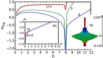
Figure 2: (color online) Impurity magnetization $m_{imp}$ vs $h$ for $J$=1, 3, and 6 in $N\!=\!72$ cluster and for $J$=1 in $N\!=\!64$ cluster (dashed). Insets: (a) Local magnetization $\Delta m_{l}^{z}\!=\!(\sin(\theta_{0})\!-\!\sin(\theta_{l}))$ in a $21{\times}21$ section of the $N\!=\!72$ cluster, for $J$=1, $h$=0.4. (b) Local magnetization $m_{l}^{z}$ at the distance ($N/2,N/2$) from $l\!=\!0$ in $N\!=\!8$ and 16 clusters for $J$=1.

Fig. 2 shows another characteristics of the texture: the impurity contribution to the uniform magnetization $m_{imp}{=}m^{z}{-}m_{host}^{z}$ vs field for several values of the coupling $J$. Here $m^{z}{=}\sum_{l}S_{l}^{z}$ is the uniform magnetization including $S^{\prime z}_{i}$ and $m_{host}^{z}{=}\sum_{l\neq i}S_{l}^{z}$ is that of the host in the absence of impurity. We use $S{=}S^{\prime}{=}1$ hereafter. Defining the impurity susceptibility as $\chi_{imp}\!=\!\partial m_{imp}/\partial h$, Fig. 2 shows several regimes of screening of the impurity by the texture: partial, complete, and overscreening, as evidenced by $\chi_{imp}\!>\!0$, $\approx\!0$, and $<\!0$, respectively. This is consistent with a field-dependent fractional effective impurity spin Wollny11 , and is in a stark contrast with the collinear HAFs, where classical $m_{imp}\!\equiv\!S^{\prime}$. The impurity magnetization is critical at $h_{s}$ because the susceptibility of the host diverges as ${\sim}\ln|h-h_{s}|$ Zhitomirsky98 . Fig. 2 also shows that the saturation in the system with impurity occurs above $h_{s}$ of the pure host and that finite-size effects are negligible for the clusters and field ranges that we use.

For completeness, we note that the impurity-induced classical texture behaves singularly at $h\!\rightarrow\!0$, although in a field range of measure zero in the thermodynamic limit — an effect also noted in Wollny12 ; weaware . In a finite system, the energy gain of the canted state in Fig. 1, $\Delta E\!\sim\!-N^{2}h^{2}/(8S)$, is less than that of the state in which the Néel order of the host and the impurity spin both fully align with the field, $\Delta E\!=\!-hS^{\prime}$. Thus, at $h\!=\!0^{+}$ host spins are aligned (anti-aligned) with the field, $S_{l}^{z}\!=\!\pm S$. A spin-flop crossover to the textured state occurs at $h_{c}\!\sim\!8SS^{\prime}/N^{2}\!\rightarrow\!0$ as $N\!\rightarrow\!\infty$. Inset (b) of Fig. 2 displays this behavior on judiciously small systems by monitoring the magnetization $m_{l}^{z}$ of a spin at the largest geometrical distance from the impurity.

$T$-matrix.—We now turn to the spectral properties of the system. Because the texture breaks translational invariance, the Bogolyubov transformation of ${\cal H}_{2}$ has to be performed numerically Colpa78 . The para-unitary, $2(N^{2}\!+\!1){\times}2(N^{2}\!+\!1)$ matrix $\mathbf{U}$ of this transformation maps the local Holstein-Primakoff bosons ${\bf a}^{\dagger}=[a_{1}^{\dagger},\dots,a_{N^{2}}^{\dagger},a_{i}^{\dagger},a_{1}^{\phantom{\dagger}},\dots,a_{N^{2}}^{\phantom{\dagger}},a_{i}^{\phantom{\dagger}}]$ onto Bogolyubov bosons $\mathbf{\bar{b}}^{\dagger}=[\bar{b}_{1}^{\dagger},\dots,\bar{b}_{N^{2}+1}^{\dagger},\bar{b}_{1}^{\phantom{\dagger}},\dots,\bar{b}_{N^{2}+1}^{\phantom{\dagger}}]$, whose Hamiltonian, ${\cal H}=\mathbf{\bar{b}}^{\dagger}\mathbf{E}\mathbf{\bar{b}}/2$, is diagonal. The eigenenergies $E_{n}$ are all positive except for $E_{j}\!=\!0$ of the Goldstone mode. The Green’s function in the $\mathbf{\bar{b}}$-basis is also a diagonal $2(N^{2}\!+\!1){\times}2(N^{2}\!+\!1)$ matrix $\mathbf{G}^{\mathbf{\bar{b}}}(z)=[z\mathbf{P}-\mathbf{E}]^{-1}$, where $\mathbf{P}$ is the para-unit matrix with $1(-1)$ in the upper (lower) half of its diagonal. The Green’s function of the local Holstein-Primakoff bosons is $\mathbf{G}^{\mathbf{a}}(z)=(\mathbf{U}^{\dagger})^{-1}\mathbf{G}^{\mathbf{\bar{b}}}(z)\mathbf{U}^{-1}$.

However, to formulate the scattering problem for the impurity-induced texture, the proper basis is that of the Bogolyubov magnons of the uniform host, which describe the incident and scattered magnons as plane-wave eigenstates of momentum $\mathbf{k}$. Thus, we first Fourier transform the matrix elements of $\mathbf{G}^{\mathbf{a}}(z)$ of the local host bosons to $\mathbf{k}$-space, yielding a matrix $\mathbf{G}^{\mathbf{a}}_{\mathbf{k}^{\prime}\mathbf{k}}(z)$. Second, the host boson terms of this matrix are mapped onto the basis of the Bogolyubov magnons ${\bf b}^{\dagger}=[b_{\mathbf{k}}^{\dagger},b_{\mathbf{k}}^{\phantom{\dagger}}]$ of the uniform host, using the known parameters of the transformation, $u_{\bf k}$ and $v_{\bf k}$, for the square-lattice HAF in a field Mourigal10 ; supp . This yields a matrix Green’s function with three $2\times 2$ substructures made from blocks of rank $N^{2}\times N^{2}$, $1$, and $N$. They correspond to the dressed (i) host magnon, (ii) impurity, (iii) and magnon-impurity Green’s functions $\mathbf{G}_{\mathbf{k}^{\prime}\mathbf{k}}(z)$, $\mathbf{G}_{i}(z)$, and $\mathbf{G}_{\mathbf{k}i}(z)$, respectively.

Altogether, starting from the numerical solution of the classical texture, followed by the real-space diagonalization of the harmonic problem, and Bogolyubov transformation onto the uniform host, we obtain the dressed magnon Green’s function $\mathbf{G}_{\mathbf{k}^{\prime}\mathbf{k}}(z)$. On the other hand, $\mathbf{G}_{\mathbf{k}^{\prime}\mathbf{k}}(z)$ can be written in the conventional form

$$\mathbf{G}_{\mathbf{k}^{\prime}\mathbf{k}}(z)=\delta_{\mathbf{k}^{\prime}\mathbf{k}}\mathbf{G}_{\mathbf{k}}^{0}(z)+\mathbf{G}_{\mathbf{k}^{\prime}}^{0}(z)\mathbf{T}_{\mathbf{k}^{\prime}\mathbf{k}}(z)\mathbf{G}_{\mathbf{k}}^{0}(z)\,,$$ (2)

where $\mathbf{G}_{\mathbf{k}}^{0}(z)$ is the diagonal $2\times 2$ Green’s function of the uniform host magnons with $G_{\mathbf{k}}^{0,11}(z)=G_{\mathbf{k}}^{0,22}(-z)=[z-\varepsilon_{\mathbf{k}}]^{-1}$ and $\varepsilon_{\mathbf{k}}$ is the magnon energy. Using Eq. (2), we can now extract the scattering matrix $\mathbf{T}_{\mathbf{k}^{\prime}\mathbf{k}}(z)$ from $\mathbf{G}_{\mathbf{k}^{\prime}\mathbf{k}}(z)$. For the remainder of this work we focus on the diagonal elements of the $T$-matrix, $\mathbf{T}_{\mathbf{k\mathbf{k}}}(z)=\mathbf{T}_{\mathbf{k}^{\prime}\mathbf{k}}(z)\delta_{\mathbf{k}^{\prime}\mathbf{k}}$

$$\mathbf{T}_{\mathbf{k}\mathbf{k}}(z)=[\mathbf{G}_{\mathbf{k}}^{0}(z)]^{-2}\mathbf{G}_{\mathbf{k}\mathbf{k}}(z)-[\mathbf{G}_{\mathbf{k}}^{0}(z)]^{-1}\,,$$ (3)

which suffice to state our main findings.

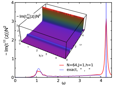
Figure 3: (color online) Analytical and numerical results for the $T$-matrix spectrum in no-texture case, $J\!=\!1$, $h\!=\!1$. Homogeneous canting angles of the host spins $\theta\!\simeq\!0.1253$. Impurity canting angle $\theta_{i}\!\simeq\!0.8729$ as in the actual texture. Thin solid blue: exact $-{\rm Im}\,t^{11}(z{=}\omega)$ supp . Impurity resonance energy at $\varepsilon\!\simeq\!1.308$, anti-bound state at $\simeq\!4.246$, van Hove singularities at $\omega_{gap}\!=\!1$ and $\omega^{max}\!\approx\!4$ are clear. Thick red solid: numerical $-{\rm Im}\,t^{11}_{{\bf k}^{\prime}{=}{\bf k}{=}0}(z{=}\omega{+}i0.05)$ for $N{=}64$. Inset: numerical $-{\rm Im}\,t^{11}_{{\bf k},{\bf k}}(z{=}\omega{+}i0.05)$ along the ${\bf k}$-path of Fig. 4.

No texture test.—First, we demonstrate the feasibility of obtaining the $T$-matrix from Eq. (3) numerically. For that purpose, we solve a complementary artificial problem, in which we neglect the feedback of the impurity on the host spins, i.e., spins in the plane retain their homogeneous field-induced canting of Fig. 1(b) and no texture is created. While such a reference state is, of course, unstable as ${\cal H}_{\mathrm{class}}$ is not at its minimum, it permits an analytical solution of the scattering problem of ${\cal H}_{2}$, details of which are provided in supp . The analytical solution can be compared to the $T$-matrix obtained from the numerical procedure described above. In the following we consider the resolvent, i.e., the $T$-matrix stripped from the matrices of the Bogolyubov basis transformation

$$\mathbf{t}_{\mathbf{k^{\prime}k}}(z)=(\mathbf{B}_{\mathbf{k^{\prime}}}^{\dagger})^{-1}\mathbf{T}_{\mathbf{k^{\prime}k}}(z)(\mathbf{B}_{\mathbf{k}})^{-1}\,,$$ (4)

where $B^{11(22)}_{\bf k}{=}u_{\bf k}$ and $B^{12(21)}_{\bf k}{=}v_{\bf k}$ supp .

The analytical result for the the resolvent spectrum, $-\textrm{Im}\,t^{11}_{{\bf k}^{\prime}{\bf k}}(z)$, is plotted in Fig. 3 vs frequency $\omega$. Naturally, $\mathbf{t}_{\mathbf{k^{\prime}k}}(z)\equiv\mathbf{t}(z)$ is momentum independent supp . This is an expected behavior for scattering from point-like defects and is similar to scattering from vacancies in collinear HAFs Brenig91 ; Chernyshev01 , where the resolvent shows some broad ${\bf k}$-modulation from superposition of a small number of partial waves. The inset of Fig. 3 shows $-\textrm{Im}\,t^{11}_{\mathbf{kk}}(z)$ obtained numerically from (3) and (4) along the path in ${\bf k}$-space shown in Fig. 4. Clearly, it is also momentum independent. In addition, analytical and numerical results, if evaluated on the finite clusters of the same size, agree to within numerical precision supp .

Finally, Fig. 3 demonstrates the spectral resolution we can obtain from the numerical procedure in an $N\!=\!64$ cluster with a minimally acceptable imaginary broadening. One can see, that the numerical scattering amplitude has all the features of the analytical one: the impurity resonance, the shallow spin-wave continuum, and the anti-bound state above the upper edge of the spectrum Fulde95 . Fine details, such as the anti-bound state gap and the non-analytic van Hove singularities are smeared out. Improving this with systems sizes beyond $N\!=\!70$ is impractical because of the large memory requirements for the non-sparse $2(N^{2}\!+\!1){\times}2(N^{2}\!+\!1)$ matrices.

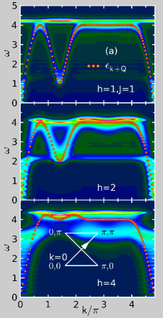
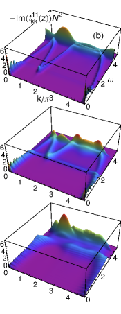
Figure 4: (color online) The $T$-matrix resolvent spectra $-{\rm Im}\,t^{11}_{{\bf k},{\bf k}}(z{=}\omega{+}i0.05)$ in $N\!=\!64$ cluster vs ${\bf k}$ and $\omega$, $J\!=\!1$, $h{=}1$, 2, and 4 along the depicted ${\bf k}$-path. Panel (a): contour plots superimposed with the shifted magnon dispersion $\varepsilon_{{\bf k}+{\bf Q}}$ (red-yellow dots). Panel (b): 3D plots.

Dispersive resonance.—We now consider the scattering $T$-matrix for the true ground state of the system with the spin texture. An analytical solution is not possible in this case. With the feasibility of the numerical procedure established, we evaluate the $T$-matrix from Eq. (3) using $\theta_{\{l\}}$ from the minimization of ${\cal H}_{\mathrm{class}}$ as an input to the Bogolyubov transformation. Representative results are shown in Fig. 4. Removing the ${\bf k}$-dependence due to transformation of the basis from $\mathbf{T}_{\mathbf{kk}}(z)$ as in (4), we show $-\textrm{Im}\,t^{11}_{{\bf k}{\bf k}}(z)$ as a function of $\omega$ and ${\bf k}$ along a high-symmetry path in the Brillouin zone and for several values of the magnetic field.

In a sharp contrast to the no-texture case, $\textrm{Im}\,t_{\mathbf{kk}}^{11}(z)$ reveals a clear dispersive feature. The localized impurity resonance in Fig. 3 is now visible only as a faint maximum and is completely overshadowed by the dispersive resonance. Such a result is completely unexpected for the point-like impurity coupled to the Heisenberg model (1). Direct comparison in Fig. 4(a) shows that the ${\bf k}$-dependence of the dispersive resonance closely follows the spinwave dispersion $\varepsilon_{\mathbf{k}+\mathbf{Q}}$, folded by the ordering vector $\mathbf{Q}=(\pi,\pi)$. As one can see, the resonance is most sharply defined for small fields and gets washed out at higher fields. We find the dispersive feature to be prominent regardless of the system size or the impurity coupling $J$.

It is reasonable to suggest that the dispersive resonance is a natural outcome of the scattering from an extended region of the impurity-induced texture, arising due to non-collinearity of the state. This can be understood qualitatively from Fig. 1(c), which shows that the impurity spin has a component that acts as a local field in the direction perpendicular to the homogeneous field-induced canting. Because of that, the spins of Fig. 1(b) are perturbed from their local reference frames by the staggered transverse effective field. Then the spin-wave part of the Hamiltonian can be written as ${\cal H}_{2}={\cal H}^{h,i}+{\cal H}^{stag}$, where ${\cal H}^{h,i}$ contains the homogeneous canting of spins and the point-like impurity scattering as in the no-texture case, while ${\cal H}^{stag}$ is inhomogeneous with staggered matrix elements, which decay on the length scale set by the texture.

Because of the staggering, magnons must experience an umklapp scattering potential that can be approximated, for an extended region of the texture, as ${\cal H}^{stag}\sim\sum_{\bf k}\mathbf{W}_{\bf k}b_{\bf k+Q}^{\dagger}b_{\bf k}^{\phantom{\dagger}}$. Here, a qualitative analogy can be drawn with the 1D Kronig-Penney model whose $T$-matrix is dispersive and has a pole close to the zone-folded band $\varepsilon_{k+Q}$ Marder . Because of the finite spatial extent of the texture, the dispersive resonance must be broadened. This is consistent with the increase of the broadening in Fig. 4 at higher fields where the size of the texture shrinks. This may imply a nontrivial behavior of the $T$-matrix in the limit of $h\rightarrow 0$ where the texture becomes quasi-long-ranged as in magnets that are non-collinear in zero field. We note that the impurity scattering does not lead to overdamping of the Goldstone mode, i.e., the spectral density at low energies in Fig. 4 does not occur at the ordering vector $\mathbf{Q}$.

Our results are of a direct relevance to the excitation spectra of non-collinear magnets with a low concentration $x$ of naturally occurring or deliberately doped impurities. Since the magnon self-energy is simply proportional to the diagonal element of the $T$-matrix via $\mathbf{\Sigma}_{\bf k}(\omega)\sim x\mathbf{T}_{\mathbf{kk}}(\omega)$, one may expect to observe an anomalous ${\bf k}$-dependent broadening of the spectrum where $\varepsilon_{\mathbf{k}}$ overlap with $\varepsilon_{\mathbf{k}+\mathbf{Q}}$ and an equally unusual field-dependence of such a broadening. These and other features should be observable by inelastic neutron scattering and specific predictions will be subject of future work.

Conclusions.—To conclude, we have presented strong evidence for a highly anomalous static and dynamic response of non-collinear antiferromagnets to doping by point-like defects. The scattering amplitude exhibits features that are strikingly different from the usual $s$-wave scattering and include a highly dispersive resonance due to an impurity-induced texture. This result should be valid for the broad class of non-collinear magnets. Further theoretical and experimental studies seem highly desirable.

Part of this work has been done at the Kavli Institute for Theoretical Physics (A.L.C. and W.B.) and at the Platform for Superconductivity and Magnetism, Dresden (W.B.). The work of A.L.C. was supported by the DOE under Grant No. DE-FG02-04ER46174. The work of W.B. was supported by DFG FOR912 Grant No. BR 1084/6-2, EU MC-ITN LOTHERM Grant No. PITN-GA-2009-238475, and the NTH SCNS. The research at KITP was supported by NSF Grant No. NSF PHY11-25915.

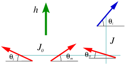
Figure 5: (color online) A sketch of the spin configuration.

.1 Classical Hamiltonian

The classical energy of the square-lattice Heisenberg AF in a field with an out-of-plane impurity, model (1) of the main text, is

$${\cal H}_{\mathrm{class}} = -S^{2}J_{0}\sum_{\langle lm\rangle}\cos(\theta_{l}+\theta_{m})-Sh\sum_{l}\sin\theta_{l}$$ (5)

$$-JSS^{\prime}\cos(\theta_{0}+\theta_{i})-hS^{\prime}\sin\theta_{i}\,,$$

where $\langle lm\rangle$ denotes bonds. The impurity site $i$ is coupled to site $l=0$ of the host and $\theta_{n}$’s are the tilt angles out of the $xy$-plane, see Fig. 5. The classical ground state is obtained by numerical minimization of ${\cal H}_{\mathrm{class}}$, i.e. by solving the set of equations $\partial{\cal H}_{\mathrm{class}}/\partial\theta_{\{l\}}=0$. The resulting spin configuration corresponds to an inhomogeneous distribution of spin canting, parametrized by the local tilt angles $\theta_{l}$, i.e. the texture. Our Fig. 6 exhibits one of the quantities that can be used to analyze the spatial extent and other characteristics of the texture: the staggered component of the magnetization $m_{stag,{\bf r}}^{z}$. The main panel displays $m_{stag,{\bf r}}^{z}$ along the $x$-axis, at location ${\bf r}=(r,0)$ off the impurity, where

$$m_{stag,{\bf r}}^{z}=(-1)^{r}\,\frac{\left(S_{(r+1,0)}^{z}-S_{(r,0)}^{z}\right)}{2}\,,$$ (6)

for two different values of impurity coupling $J$ and for various field strengths. The impurity is coupled to site $R=(0,0)$ of a cluster with $N=70$. Clearly, the spatial extent of the texture increases as the field $h\!\rightarrow\!0$. Inset (a) demonstrates that the texture decays exponentially commentAccuracy at $r\gg 1$. This behavior is expected because the impurity is not coupled to the Goldstone mode of the host. This finding is consistent with earlier work Eggert07a where $m_{stag,{\bf r}}^{z}$ was investigated for a different type of impurity (vacancy) by a continuum theory and quantum Monte Carlo. We do not observe exact exponential behavior in the low-field regime, most likely because of the finite cluster size. By varying $h$ we find that $m_{stag,{\bf r}}^{z}/h$ scales almost perfectly with $r\cdot h$, see inset (b) of Fig. 6, again in agreement with Eggert07a . One potential reason for the visible deviation from scaling is the field dependence of the transverse susceptibility $\chi_{\perp}$ and the spin stiffness $\rho_{s}$, neglected in the continuum description of Eggert07a .

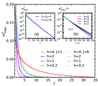
Figure 6: (color online) The staggered component of magnetization $m_{stag,{\bf r}}^{z}$ (6) vs distance $r$ from the origin for two different values of impurity coupling $J$ and for various field strengths. The impurity is coupled to site $R=(0,0)$ of a cluster with $N=70$. Inset (a) same on the semi-log plot. Inset (b) $m_{stag,{\bf r}}^{z}/h$ vs $r\cdot h$.

.2 Harmonic part of the Hamiltonian

Within the $1/S$ expansion, the local spin quantization axes on each site are aligned in the direction given by the local canted frame with the angle $\theta_{l}$, obtained from the minimization of the classical energy. The subsequent Holstein-Primakoff bosonization of spin operators yields the harmonic spin-wave Hamiltonian ${\cal H}_{2}$. The term linear in bosonic operators, ${\cal H}_{1}$, vanishes identically upon minimization of ${\cal H}_{\mathrm{class}}$.

The spin-wave Hamiltonian of the host reads

$${\cal H}^{\rm host}_{2}=J_{0}S\sum_{l,\delta}\bigg{\{}\cos\theta_{l\delta}\ a^{\dagger}_{l}a^{\phantom{{\dagger}}}_{l}+\sin^{2}\frac{\theta_{l\delta}}{2}\ a^{\dagger}_{l}a^{\phantom{{\dagger}}}_{l+\delta}$$ (7)

$$\phantom{{\cal H}_{2}}-\frac{1}{2}\,\cos^{2}\frac{\theta_{l\delta}}{2}\left(a^{\dagger}_{l}a^{{\dagger}}_{l+\delta}+{\rm H.c.}\right)\bigg{\}}+h\sum_{l}\sin\theta_{l}\ a^{\dagger}_{l}a^{\phantom{{\dagger}}}_{l}\,,$$

where the summation is over the lattice sites $l$ and the nearest neighbors $\delta$ and the shorthand notation $\theta_{l\delta}=\theta_{l}+\theta_{l+\delta}$ has been introduced. The impurity part of the Hamiltonian is

$${\cal H}^{\rm imp}_{2} = J\cos\theta_{0i}\left(S\,a^{\dagger}_{0}a^{\phantom{{\dagger}}}_{0}+S^{\prime}\,a^{\dagger}_{i}a^{\phantom{{\dagger}}}_{i}\right)+h\,\sin\theta_{i}\ a^{\dagger}_{i}a^{\phantom{{\dagger}}}_{i}$$

$$+ J\sqrt{SS^{\prime}}\bigg{\{}\sin^{2}\frac{\theta_{0i}}{2}\left(a^{\dagger}_{0}a^{\phantom{{\dagger}}}_{i}+{\rm H.c.}\right)$$

$$\phantom{J\sqrt{SS^{\prime}}\bigg{\{}}-\cos^{2}\frac{\theta_{0i}}{2}\left(a^{\dagger}_{0}a^{{\dagger}}_{i}+{\rm H.c.}\right)\bigg{\}},$$

where $\theta_{0i}=\theta_{0}+\theta_{i}$. The first line contains a potential-like energy shift for the magnon on the site coupled to the impurity ($l=0$) and the local energy of the impurity magnon, while the rest of the Hamiltonian describes various transitions between the two.

In the textured case, analytical diagonalization of the Hamiltonian (7) and (.2) is not feasible, so we perform the Bogolyubov transformation numerically. Subsequently, the $T$-matrix is extracted from the Green’s function written in the basis of Bogolyubov magnons of the uniform system (no impurity), as described in the main text.

.3 No texture test

The feasibility of extracting the $T$-matrix from the full Green’s function numerically can be demonstrated for a complementary artificial problem, for which an analytical solution can also be found, and by comparing the results of the two approaches. Here we formulate such a problem by neglecting the feedback of the impurity onto the host spins, so that no texture is created. While such a reference state is unstable as ${\cal H}_{\mathrm{class}}$ is not minimal, it permits an analytical solution of the scattering problem.

.3.1 Hamiltonian

In the no-texture case, the canting of the host spins is uniform, $\theta_{l}=\theta$, with the canting angle found from the energy minimization of the system without impurity: $\sin\theta=h/h_{s}$ with the saturation field $h_{s}=8SJ_{0}$. The subsequent diagonalization of the host Hamiltonian (7) is straightforward Zhitomirsky98a ; Mourigal10a and leads to

$${\cal H}^{\rm host}_{2}=\sum_{\bf{k}}\varepsilon_{\bf{k}}b_{\bf{k}}^{\dagger}b_{\bf{k}}^{\phantom{\dagger}},$$ (9)

where $\varepsilon_{\bf{k}}=4SJ_{0}\sqrt{(1+\gamma_{\bf{k}})(1-\gamma_{\bf{k}}\cos 2\theta)}$ is the spin-wave dispersion and $\gamma_{\bf{k}}=\frac{1}{2}(\cos k_{x}+\cos k_{y})$. The Bogolyubov transformation from $a_{\bf k}^{\dagger}=\frac{1}{N}\sum_{l}e^{i{\bf k}\cdot\mathbf{r}_{l}}a_{l}^{{\dagger}}$ to $b^{\phantom{{\dagger}}}_{\bf{k}}$ and $b_{\bf{k}}^{\dagger}$ is written as

$$\Phi_{\bf k}=\mathbf{B_{\bf k}}\Psi_{\bf{k}}\,,$$ (10)

where

$$\Phi_{\bf k}=\left[\begin{array}[]{c}a_{\bf k}^{\phantom{{\dagger}}}\\ a_{-\bf k}^{{\dagger}}\end{array}\right],\ \ \Psi_{\bf{k}}=\left[\begin{array}[]{c}b_{\bf k}^{\phantom{{\dagger}}}\\ b_{-\bf k}^{{\dagger}}\end{array}\right],\ \ \mathbf{B_{\bf k}}=\left[\begin{array}[]{cc}u_{\bf k}&v_{\bf k}\\ v_{\bf k}&u_{\bf k}\end{array}\right],\ \ \ \ \ \$$ (17)

is a convenient $2\times 2$ notation. The $u$-$v$ factors are: $u_{\bf k}=\sqrt{(A_{\bf k}+\varepsilon_{\bf k})/2\varepsilon_{\bf k}}$, $v_{\bf k}=\mathrm{sign}(\gamma_{\bf k})\sqrt{(A_{\bf k}-\varepsilon_{\bf k})/2\varepsilon_{\bf k}}$, with $A_{\bf k}=4SJ_{0}(1+\gamma_{\bf k}\sin^{2}\theta)$ Zhitomirsky98a ; Mourigal10a .

Using these notations and that ${\bf B}_{\bf k}={\bf B}_{\bf k}^{\dagger}$, the impurity part of the spin-wave Hamiltonian (.2) can be written as

$${\cal H}^{\rm imp}_{2} = \varepsilon\,a_{i}^{{\dagger}}a_{i}^{\phantom{{\dagger}}}+\frac{V_{0}}{2}\sum_{\bf k,k^{\prime}}\Psi_{\bf k^{\prime}}^{{\dagger}}{\bf B}_{\bf k^{\prime}}{\bf B}_{\bf k}\Psi_{\bf k}^{\phantom{{\dagger}}}+\sum_{\bf k}\Psi_{\bf k}^{\dagger}{\bf B}_{\bf k}{\bf V}_{1}\Phi_{i}^{\phantom{\dagger}},$$

$${\rm with} \Phi_{i}=\left[\begin{array}[]{c}a_{i}^{\phantom{{\dagger}}}\\ a_{i}^{{\dagger}}\end{array}\right],\ \ \ \ {\bf V}_{1}=V_{1}\left[\begin{array}[]{cc}f&g\\ g&f\end{array}\right],$$ (22)

where potential-like scattering amplitude $V_{0}\!=\!JS\cos\theta_{0i}$, magnon-impurity transfer amplitude $V_{1}\!=\!J\sqrt{SS^{\prime}}$, matrix elements $f\!=\!\sin^{2}(\theta_{0i}/2)$ and $g\!=\!-\cos^{2}(\theta_{0i}/2)$, and the angle $\theta_{0i}\!=\!\theta\!+\!\theta_{i}$ as before. With the notations (17), the last term of the magnon-impurity scattering in (22) implicitly contains its own conjugate. The impurity energy is $\varepsilon\!=\!JS^{\prime}\cos\theta_{0i}\!+\!h\sin\theta_{i}$ with an impurity canting angle $\theta_{i}$ which is a free parameter. In the following, we fix the latter to its value obtained numerically for the problem with the texture. One might also chose $\theta_{i}$ to minimize the energy of the impurity spin in (5) while keeping the host canting angle homogeneous. This yields $\tan\theta_{i}\!=\!(8J_{0}/J\!-\!1)\tan\theta$, which is numerically close to the problem with the texture.

.3.2 Green’s function and $T$-matrix

The imaginary time Green’s function of the $b^{({\dagger})}_{\bf{k}}$ magnons is a $2\!\times\!2$ matrix which can be written as a direct product ${\bf G}_{\bf k^{\prime}\bf k}(\tau)\!=\!-\langle T_{\tau}(\Psi_{\bf k^{\prime}}^{\phantom{\dagger}}(\tau)\!\otimes\!\Psi_{\bf k}^{\dagger})\rangle$ using (17). Its Fourier transform is ${\bf G}_{\bf k^{\prime}\bf k}(i\omega_{n})\!=\!\int_{0}^{\beta}\exp(i\omega_{n}\tau){\bf G}_{\bf k^{\prime}\bf k}(\tau)d\tau$, where $i\omega_{n}\!=\!i2n\pi T$, which we replace by a complex variable $z$ hereafter. The Green’s function in the presence of impurity scattering can be expressed through the $T$-matrix

$${\bf G}_{\bf k^{\prime}\bf k}(z) = \delta_{\bf k^{\prime}\bf k}{\bf G}_{\bf k}^{0}(z)+{\bf G}_{\bf k^{\prime}}^{0}(z){\bf T}_{\bf k^{\prime}\bf k}(z){\bf G}_{\bf k}^{0}(z)\,,$$ (23)

where the noninteracting Green’s function ${\bf G}_{\bf k}^{0}(z)$ is

$${\bf G}_{\bf k}^{0}(z) = \left[\begin{array}[]{cc}\frac{1}{z-\varepsilon_{\bf k}}&0\\ 0&-\frac{1}{z+\varepsilon_{\bf k}}\end{array}\right]\,.$$ (26)

Using the impurity scattering terms in (22), the $T$-matrix follows from an infinite sequence of the two-component vertex function, one component from the potential-like scattering $V_{0}$-term and the other from the magnon-impurity scattering $V_{1}$-term. Figs. 7(a) and (b) show the vertex and the sequence, respectively. From the structure of the vertex

$$\mathbf{\Gamma}_{\bf k^{\prime}\bf k}(z)={\bf B}_{\bf k^{\prime}}^{\dagger}\mathbf{\Gamma}(z){\bf B}_{\bf k}\,,$$ (27)

where the ${\bf k}$-independent vertex is

$$\mathbf{\Gamma}(z)=V_{0}{\bf 1}+{\bf V}_{1}{\bf G}_{i}^{0}(z){\bf V}_{1}\,,$$ (28)

and ${\bf G}_{i}^{0}(z)$ is the local Green’s function of the impurity state,

$${\bf G}_{i}^{0}(z)=\left[\begin{array}[]{cc}\frac{1}{z-\varepsilon}&0\\ 0&-\frac{1}{z+\varepsilon}\end{array}\right],$$ (31)

it is straightforward to see that the $T$-matrix has no ${\bf k}$-dependence aside from the trivial basis change ${\bf B}_{\bf k}$ and ${\bf B}_{\bf k^{\prime}}$ to Bogolyubov bosons

$${\bf T}_{\bf k^{\prime}\bf k}(z)={\bf B}_{\bf k^{\prime}}^{\dagger}{\bf t}(z){\bf B}_{\bf k}\,.$$ (32)

This is a standard feature, not only for the particular type of impurity in antiferromagnets that we investigate, but for the point-like scatterers in general. Stated differently, the actual scattering resolvent ${\bf t}(z)$ is completely momentum independent. Using (27), (28), and Fig. 7(b) one readily arrives at the final expression for the resolvent

$${\bf t}(z)=\frac{\mathbf{\Gamma}(z)}{{\bf 1}-{\bf F}(z)\mathbf{\Gamma}(z)}\,,$$ (33)

where the matrix ${\bf F}(z)$

$${\bf F}(z)=\left[\begin{array}[]{cc}G_{0}(z)&F_{0}(z)\\ F_{0}(z)&G_{0}(-z)\end{array}\right],$$ (36)

is built from the local Holstein-Primakoff Green’s functions of the host

$$G_{0}(z) = \sum_{\bf k}\left(\frac{u_{\bf k}^{2}}{z-\varepsilon_{\bf k}}-\frac{v_{\bf k}^{2}}{z+\varepsilon_{\bf k}}\right)$$

$$F_{0}(z) = \sum_{\bf k}\left(\frac{v_{\bf k}u_{\bf k}}{z-\varepsilon_{\bf k}}-\frac{u_{\bf k}v_{\bf k}}{z+\varepsilon_{\bf k}}\right)\,.$$ (37)

This concludes the formal solution of the scattering problem. The remaining step is the momentum integration in $G_{0}(z)$ and $F_{0}(z)$. In the next section, we summarize our analytical results for this integration.

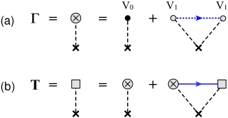
Figure 7: (color online) (a) Composite vertex of impurity scattering in (22). (b) $T$-matrix sequence with that vertex. Dotted and solid lines are the noninteracting impurity resonance and the host magnon Green’s functions, respectively.

.3.3 Local Green’s functions

Since in the scattering problem we are interested in the retarded $T$-matrix, we need to evaluate $G_{0}(z)$ and $F_{0}(z)$ in (37) for $z=\omega+i0^{+}$. Both Green’s functions have real and imaginary parts:

$$G_{0}(\omega) = G^{\prime}_{0}(\omega)+iG^{\prime\prime}_{0}(\omega)$$

$$F_{0}(\omega) = F^{\prime}_{0}(\omega)+iF^{\prime\prime}_{0}(\omega)\,.$$ (38)

It is convenient to express all energies in units of the zero-field magnon bandwidth, $W_{0}=4J_{0}S$, and the field in units of the saturation field of the host, $h_{s}=8J_{0}S$. Thus, in the following $\bar{h}=h/h_{s}$ and $\bar{\omega}=\omega/4J_{0}S$. Three other energy scales are needed for the results below: the field-dependent gap in the magnon spectrum

$$\bar{\omega}_{g}=\frac{\omega_{gap}}{4J_{0}S}=2\bar{h},$$ (39)

an auxiliary scale

$$\bar{\omega}_{m}=\frac{\omega_{m}}{4J_{0}S}=\frac{1-\bar{h}^{2}}{\sqrt{1-2\bar{h}^{2}}},$$ (40)

and the field-dependent magnon bandwidth

$$\frac{W}{4J_{0}S}=\begin{cases}\bar{\omega}_{m},&\bar{h}\leq 1/\sqrt{3}\\ \bar{\omega}_{g},&\bar{h}\geq 1/\sqrt{3}\,.\end{cases}$$ (41)

For $-W<\omega<W$, and after some algebra, we arrive at the following expressions for the imaginary parts

$$G^{\prime\prime}_{0}(\omega)=\frac{-1}{\pi W_{0}r(\bar{\omega})}\bigg{[}\Theta\left(\bar{\omega}^{2}-\bar{\omega}_{g}^{2}\right)\left(1+\bar{\omega}+\bar{h}^{2}\gamma_{1}\right)K\left(\gamma^{\prime}_{1}\right)$$

$$\phantom{G^{\prime\prime}_{0}(\omega)=\frac{-1}{\pi W_{0}r(\bar{\omega})}\bigg{[}}+\left(1+\bar{\omega}+\bar{h}^{2}\gamma_{2}\right)K\left(\gamma^{\prime}_{2}\right)\bigg{]},$$ (42)

$$F^{\prime\prime}_{0}(\omega)=\frac{-(1-\bar{h}^{2})}{\pi W_{0}r(\bar{\omega})}\bigg{[}\Theta\left(\bar{\omega}^{2}-\bar{\omega}_{g}^{2}\right)\gamma_{1}K\left(\gamma^{\prime}_{1}\right)+\gamma_{2}K\left(\gamma^{\prime}_{2}\right)\bigg{]}.$$

The expressions for the real parts of the local Green’s functions for the same energy range $-W<\omega<W$ are complimentary to (42)

$$G^{\prime}_{0}(\omega)=\frac{-1}{\pi W_{0}r(\bar{\omega})}\bigg{[}\Theta\left(\bar{\omega}^{2}-\bar{\omega}_{g}^{2}\right)\left(1+\bar{\omega}+\bar{h}^{2}\gamma_{1}\right)K\left(\gamma_{1}\right)$$

$$\phantom{G^{\prime}_{0}(\omega)=\frac{-1}{\pi}}+\Theta\left(\bar{\omega}_{g}^{2}-\bar{\omega}^{2}\right)\left(1+\bar{\omega}+\bar{h}^{2}\gamma_{1}\right)\frac{1}{\gamma_{1}}K\left(\frac{1}{\gamma_{1}}\right)$$

$$\phantom{G^{\prime}_{0}(\omega)=\frac{-1}{\pi}}-{\rm sign}\left(\gamma_{2}\right)\left(1+\bar{\omega}+\bar{h}^{2}\gamma_{2}\right)K\left(\gamma_{2}\right)\bigg{]},$$ (43)

$$F^{\prime}_{0}(\omega)=\frac{-(1-\bar{h}^{2})}{\pi W_{0}r(\bar{\omega})}\bigg{[}\Theta\left(\bar{\omega}^{2}-\bar{\omega}_{g}^{2}\right)\gamma_{1}K\left(\gamma_{1}\right)$$

$$\phantom{F^{\prime}_{0}(\omega)=}+\Theta\left(\bar{\omega}_{g}^{2}-\bar{\omega}^{2}\right)K\left(\frac{1}{\gamma_{1}}\right)-{\rm sign}\left(\gamma_{2}\right)\gamma_{2}K\left(\gamma_{2}\right)\bigg{]},$$

where $\Theta$’s are step-functions, $K$’s are complete elliptic integrals of the first kind, $\gamma^{\prime}_{i}=\sqrt{1-\gamma_{i}^{2}}$, and

$$\gamma_{1,2}=\frac{\bar{h}^{2}\pm r(\bar{\omega})}{1-2\bar{h}^{2}},$$ (44)

are the roots of the equation $\bar{\omega}^{2}-\bar{\omega}_{\bf k}^{2}=0$, i.e.

$$r(\bar{\omega})=\sqrt{\left(1-2\bar{h}^{2}\right)\left(\bar{\omega}^{2}_{m}-\bar{\omega}^{2}\right)}\,.$$ (45)

One may notice, that for the field $\bar{h}>1/\sqrt{3}$ some of the step-functions [$\Theta\left(\bar{\omega}^{2}-\bar{\omega}_{g}^{2}\right)$] are zero in the considered energy range $\omega^{2}<W^{2}$, because $W=\omega_{gap}$ for this field range. As a consequence, some of the terms in (42) and (43) vanish entirely for that field range.

For energies outside the magnon bandwidth, $\omega^{2}>W^{2}$, the imaginary parts of $G_{0}$ and $F_{0}$ are identically zero. The derivation of the real parts, while somewhat more convoluted, eventually leads to two cases. First,

$$G^{\prime}_{0}(\omega)=-\frac{2}{\pi W_{0}r_{1}(\bar{\omega})}{\rm Im}\bigg{[}\left(1+\bar{\omega}+\bar{h}^{2}\gamma_{1}\right)\frac{1}{\gamma_{1}}K\left(\frac{1}{\gamma_{1}}\right)\bigg{]},$$

$$F^{\prime}_{0}(\omega)=-\frac{2(1-\bar{h}^{2})}{\pi W_{0}r_{1}(\bar{\omega})}{\rm Im}\bigg{[}K\left(\frac{1}{\gamma_{1}}\right)\bigg{]},$$ (46)

with

$$r_{1}(\bar{\omega})=\sqrt{\left(1-2\bar{h}^{2}\right)\left(\bar{\omega}^{2}-\bar{\omega}_{m}^{2}\right)}\,.$$ (47)

This is valid for fields within the range $\bar{h}\leq 1/\sqrt{3}$ for any $\omega^{2}>W^{2}$ and for $1/\sqrt{3}<\bar{h}\leq 1/\sqrt{2}$ for $\omega^{2}>\omega^{2}_{m}$ ($\omega^{2}_{m}>W^{2}$). Second,

$$G^{\prime}_{0}(\omega)=-\frac{1}{\pi W_{0}r(\bar{\omega})}\bigg{[}\left(1+\bar{\omega}+\bar{h}^{2}\gamma_{1}\right)\frac{1}{\gamma_{1}}K\left(\frac{1}{\gamma_{1}}\right)$$

$$\phantom{G^{\prime}_{0}(\omega)=-\frac{1}{\pi}W_{0}}-\left(1+\bar{\omega}+\bar{h}^{2}\gamma_{2}\right)\frac{1}{\gamma_{2}}K\left(\frac{1}{\gamma_{2}}\right)\bigg{]},$$ (48)

$$F^{\prime}_{0}(\omega)=-\frac{(1-\bar{h}^{2})}{\pi W_{0}r(\bar{\omega})}\bigg{[}K\left(\frac{1}{\gamma_{1}}\right)-K\left(\frac{1}{\gamma_{2}}\right)\bigg{]},$$

which is valid for fields within the range $1/\sqrt{3}<\bar{h}\leq 1$ for any $\omega^{2}>W^{2}$ and for the fields $1/\sqrt{3}<\bar{h}\leq 1/\sqrt{2}$ for $\omega^{2}_{m}<\omega^{2}<W^{2}$.

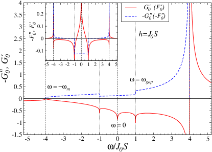
Figure 8: (color online) Real and imaginary parts of $G_{0}(\omega)$ and $F_{0}(\omega)$ for $h=J_{0}S$ ($\bar{h}=0.125$).

Fig. 8 shows the real and imaginary parts of $G_{0}$ and $F_{0}$ for a representative choice of $h=J_{0}S$ ($\bar{h}=0.125$). Pronounced van Hove singularities at the top of the magnon spectrum ($W\approx 4J_{0}S$) and at the field-induced gap ($\omega_{gap}=h$) are clearly visible. These nonanalyticities are present in the $\omega$-dependence of the analytical result for $-{\rm Im}\,t^{11}(\omega)$ from (33), which is depicted in Fig. 3 of the main text, but are much less pronounced.

.3.4 Comparison of analytical and numerical results

The analytical solution of the artificial problem can also be used to check the numerical solution beyond the discussion in the main text. To this end, rather than performing the integration in (37) exactly, the momentum sum is carried out numerically on a finite cluster of the same size as the one used in the numerical procedure. The resulting two $T$-matrices can then be compared. A typical case is shown in Fig. 9, where we depict the relative difference of the diagonal elements $t^{11}(z)$ of the resolvents obtained from each of the two approaches, versus frequency for a finite $N\times N$ cluster with $N=64$, exchanges $J=J_{0}=1$, spins $S=S^{\prime}=1$, and field $h=2$. For this plot, the imaginary broadening in $z=\omega+i\eta$ has been set to $\eta=0.005$. For this system size and the choice of parameters, such value of $\eta$ is small enough, so that each individual delta-function in the spectrum, corresponding to every single eigenenergy, is resolved. Therefore, this figure demonstrates an agreement between the two approaches not only to within the precision of the linear algebra routines that are used for the numerical Bogolyubov transformation, but also on a level of resolution down to each individual eigenstate.

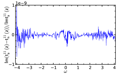
Figure 9: (color online) The relative difference between the imaginary part of the analytical ($a$) and numerical ($n$) resolvents $t^{11}(z)$ for the finite $N\times N$ cluster with $N=64$, exchanges $J=J_{0}=1$, spins $S=S^{\prime}=1$, field $h=2$, and $z=\omega+i\eta$ with $\eta=0.005$. For these parameters, the uniform canting angle is $\theta=0.2527$ and the impurity canting angle is $\theta_{i}=1.122$.

References

(1) P. W. Anderson, Phys. Rev. 109, 1492 (1958).
(2) A. A. Abrikosov and L. P. Gorkov, Sov. Phys. JETP 12,
1243 (1961) [ZhETF 39(6), 1781 (1960)].
(3) P. W. Anderson, Phys. Rev. Lett. 18, 1049 (1967).
(4) O. P. Vajk, P. K. Mang, M. Greven, P. M. Gehring, and J. W. Lynn,
Science 295, 1691 (2002).
(5) A. W. Sandvik, Phys. Rev. Lett. 89, 177201 (2002).
(6) T. Vojta and J. Schmalian, Phys. Rev. Lett. 95, 237206 (2005).
(7) R. Yu, T. Roscilde, and S. Haas, Phys. Rev. Lett. 94, 197204 (2005).
(8) A. W. Sandvik, Phys. Rev. Lett. 96, 207201 (2006).
(9) G. B. Martins, M. Laukamp, J. Riera, and E. Dagotto,
Phys. Rev. Lett. 78, 3563 (1997).
(10) S. Sachdev, C. Buragohain, and M. Vojta, Science 286, 2479
(1999).
(11) K. H. Höglund and A. W. Sandvik, Phys. Rev. Lett. 91,
077204 (2003).
(12) W. Brenig and A. P. Kampf, Phys. Rev. B 43,12914 (1991).
(13) A. L. Chernyshev, Y. C. Chen, and A. H. Castro Neto,
Phys. Rev. Lett. 87, 067209 (2001); Phys. Rev. B 65, 104407 (2002).
(14) S. Dommange, M. Mambrini, B. Normand, and F. Mila, Phys. Rev. B
68, 224416 (2003).
(15) G. B. Martins and W. Brenig, J. Phys.: Cond. Matt. 20,
415204 (2008).
(16) C. Weber and F. Mila, preprint, arXiv:1207.0095.
(17) R. R. P. Singh, Phys. Rev. Lett. 104, 177203 (2010).
(18) D. Poilblanc and A. Ralko, Phys. Rev. B 82, 174424 (2010).
(19) A. J. Willans, J. T. Chalker, and R. Moessner, Phys. Rev. B
84, 115146 (2011).
(20) A. Wollny, E. C. Andrade, and M. Vojta, Phys. Rev. Lett. 109,
177203 (2012).
(21) S. Eggert, O. F. Syljuåsen, F. Anfuso, and M. Andres,
Phys. Rev. Lett. 99, 097204 (2007).
(22) A. Wollny, L. Fritz, and M. Vojta, Phys. Rev. Lett. 107,
137204 (2011).
(23) C. Henley, Can. J. Phys. 79, 1307 (2001).
(24) A. Lüscher and O. P. Sushkov, Phys. Rev. B 71, 064414
(2005).
(25) M. E. Zhitomirsky and T. Nikuni, Phys. Rev. B 57, 5013
(1998).
(26) M. Mourigal, M. E. Zhitomirsky, and A. L. Chernyshev, Phys. Rev. B
82, 144402 (2010).
(27) See Supplemental Material at http://link.aps.org/supplemental for
details of the calculations of the static and dynamical properties of the model (1).
(28) After completion of our work, we became aware of the study
Wollny12 , reporting similar findings but for different types of host spin systems
and impurities.
(29) J. H. P. Colpa, Physica A 93, 327 (1978).
(30) J. Igarashi, K. Murayama, and P. Fulde, Phys. Rev. B 52, 15966
(1995).
(31) M. P. Marder, Condensed Matter Physics, (Wiley, New Jersey, 2010).

References

(1)
We have set the global error in the steepest decent for to be
less than .
(2) S. Eggert, O. F. Syljuåsen, F. Anfuso, and M. Andres,
Phys. Rev. Lett. 99, 097204 (2007).
(3) M. E. Zhitomirsky and T. Nikuni, Phys. Rev. B 57, 5013
(1998).
(4) M. Mourigal, M. E. Zhitomirsky, and A. L. Chernyshev, Phys. Rev. B
82, 144402 (2010).