The Mass Function of Primordial Rogue Planet MACHOs in quasar nanolensing

Abstract

The recent Sumi et al (2010, 2011) detection of free roaming planet mass MACHOs in cosmologically significant numbers recalls their original detection in quasar microlening studies (Schild 1996, Colley and Schild 2003). We consider the microlensing signature of such a population, and find that the nano-lensing (microlensing) would be well characterized by a statistical microlensing theory published previously by Refsdal and Stabel (1991). Comparison of the observed First Lens microlensing amplitudes with the theoretical prediction gives close agreement and a methodology for determining the slope of the mass function describing the population. Our provisional estimate of the power law exponent in an exponential approximation to this distribution is $2.98^{+1.0}_{-0.5}.$ where a Salpeter slope is 2.35.

1 Introduction

The recent detection of planetary mass MACHOS seen in high-cadence searches toward the Galactic Center and the Large Magellanic Cloud (LMC) (Sumi et al, 2010, 2011) suggest that a significant population of dark planet-mass MACHOs populate the halo of our Galaxy, which may constitute the Galactic dark matter. This would (partly) explain the “missing baryon problem”, the fact that about 90% of the baryons in the solar neighborhood are unaccounted for. Indeed, below we clarify this from similar detections made in last decades with micro-lensing and even nano-lensing in the Q0957+561 A,B gravitational lens system (the so-called First Lens). Insofar as the observed MACHOs are planetary mass bodies dominated by hydrogen and 26% in weight of helium, other modes of their detection as extreme scattering events seen in the line of sight to ordinary quasars, and as the sources of the ubiquitous “dust” emission at temperatures of minimally 15 K and of the “mysterious radio events”, may also be signaling their detection (Nieuwenhuizen et al 2010).

In the following we re-consider the expected microlensing signature, optical depths, and mass spectrum of the observed planet mass MACHO population. Presently there is confusion in the literature about what to call these objects, because there is increasing awareness from emerging statistics of ubiquity of orbiting planets accompanying ordinary stars that the many orbital interactions should frequently result in escape from the initial orbiting planetary systems. To avoid confusion, we call free-roaming planetary mass condensed objects “escapees” if originally formed in pre-stellar accretion discs, and “micro brown dwarfs” ($\mu$BDs) if formed primordially by gas fragmentation. Of course we still call ordinary star-orbiting bodies planets.

1.1 Quasar Microlensing and the missing baryons problem

The existence of a population of planet mass microlensing objects, also called MACHOs, was first inferred from quasar microlensing studies by Schild (1996) when it was discovered that no value close to the accepted time delay would remove the pattern of daily sampled quasar brightness fluctuations. The subject was complicated by the fact that to securely recognize the signal, it would be necessary to measure the double image quasar time delay to a fraction of a day. This was accomplished by an international around-the-world consortium (Colley et al, 2002, 2003) whose 417.1-day time delay value still stands as the most precise time delay ever measured. Re-analysis of an earlier observation of 5 consecutive nights of continuous brightness monitoring data produced a microlensing event of duration 5 hours (quasar proper time), by Colley and Schild, (2003).

Such rapid events can realistically be understood only as resulting from microlensing. Recall that a quasar is approximately 100 times brighter than our Milky Way galaxy. If attributed to the quasar, the observed 1 percent brightness fluctuation in the quasar light is energetically equivalent to the entire Milky Way luminosity being switched on and off in only 5 hours – which is an implausible scenario. For observation from the earth, the intensity fluctuation can be accomplished by the gravitational field of a microlensing compact object. Indeed, an observed negative brightness change is in fact a re-direction of the 1% part of the enormous luminosity away from the line of sight of the affected quasar image. Likewise, a positive 1% change is due to a lensing effect that focuses more light in the observer’s direction.

The original rapid microlensing detection was greeted with strong interest, because it was immediately recognized that it could not be caused by stars (Catalano 1997). Since it was obviously seen as a continuous brightness fluctuation pattern at approximately unit optical depth, it must represent the detection of the dark baryonic matter. But the interest faded away when the EROS and MACHO consortia did not observe similar MACHOs in front of the Magellanic Clouds. However, the quasar data themselves have never been questioned and related effects were observed on other, lensed quasars, as commonly discussed in the context of measurement of time delay (Burud et al, 2000, 2002; Paraficz et al, 2006, Vakulik et al, 2007, 2008). To settle this dispute, we intend to redo a search in front of the Large Magellanic Cloud (Schild et al, 2012).

To explain the quasar observations, other possibilities than MACHOs were considered as well, such as hypothetical orbiting luminous blobs in the accretion disc, for which, however, there had never previously been evidence (Gould and Miralda-Escude, 1996). Finally, a series of simulations of orbiting luminous blobs and obscuring clouds by Wyithe and Loeb (2002) produced brightness curves that could be compared to observations. Simulations for orbiting dark spots and bright spots microlensed by patterns of cusps originating in the lens galaxy show that the longer duration events have smaller brightness amplitudes than shorter duration events (Figure 6). But the wavelet analysis of the observed microlensing brightness fluctuations by Schild (1999) consistently showed an opposite pattern of larger brightness fluctuation amplitude for longer duration events. Moreover, in general the simulated brightness curves do not look like the observational results, and in particular do not show the observed feature of equal positive and negative events (Schild 1999).

An additional simulation showed that for the process championed by Schild (1996), with quasar structure microlensed by cusps originating in the lens galaxy, larger amplitude brightness effects were always found for longer duration events (Wyithe and Loeb, 2002, Fig. 9). The wavelet analysis of the microlensing brightness fluctuations by Schild (1999) consistently showed this pattern of larger brightness amplitude for longer duration events.

Since the Wyithe and Loeb (2002) simulation only covered stellar to Jupiter microlensing masses and not to the Earth masses or smaller, as implied by the Colley and Schild (2003) event, the targeted simulation by Schild and Vakulik (2003) for The First Lens, Q0957, is of more relevance. It demonstrates microlensing events caused not by orbiting blobs, but rather by a drift pattern of microlensing cusps originating in the lens galaxy and microlensing the discrete luminous quasar structures, creating a continuous pattern of brightness cusps at the observed $1\%$ level with event durations of a few days, caused by microlens masses $10^{-5}M_{\odot}$.

Thus in this paper we return to the interpretation of the quasar microlensing effect as due to a population of MACHOs. In the following sections we will first consider in section 2 the statistics describing the probability of microlensing in the quasar lens system, and then in section 3 we show how the theory of microlensing for large luminous sources gives an excellent fit to the observed amplitude of brightness fluctuations. In section 4 we demonstrate a technique for determination of the mass function describing the observed masses of the rogue planet MACHOs. We summarize our conclusions in section 5.

2 Quasar structure and microlensing observations

2.1 On size scales of luminous quasar structure inferred from microlensing

Technically speaking, the subject of lensing by individual objects within a resolved object like a distribution of stars in a lens galaxy foreground to a distant quasar is discussed under the topic of microlensing, although if the grainey distribution is composed of planet mass objects, it would more correctly be described as nano-lensing. We follow standard usage and simply adopt the word microlensing in this report.

It is also important to understand that the microlensing by planet mass objects resolves the structure of the central regions of quasars, taken to be black hole or MECO objects (Schild, Leiter, and Robertson 2006; SLR06). For one such object, the doubly imaged quasar Q0957+561 the distance observed between the A and B images is 6.26 arcsec. It has redshift of source $z_{S}=1.43$ and of the lens $z_{L}=0.355$, the BH mass is $3.6\,10^{9}M_{\odot}$ (SLR06) and the gravitational radius $R_{G}=GMc^{-2}$ is $5.3\cdot 10^{14}$ cm.

We describe the luminour ring at the inner edge of the accretion disc as a torus having two radii of importance; the outer radius, which refers to the quasar central radius to the inner edge of the accretion disc, and the sectional radius, which is half the thickness of the accretion disc and therefore the cross sectional radius. Then the outer radius is $R_{\rm outer}=74\,R_{G}=3.94\,10^{16}$ cm and the sectional radius is $R_{\perp}^{\prime}=1.52\cdot 10^{13}$ cm. The main part of the quasar light comes from a structure of this radius. We adopt the standard cosmology with $H_{0}=70$ km/s Mpc, $\Omega_{c}=0.23$, $\Omega_{B}=0.05$, so that $\Omega_{M}=0.28$, and $\Omega_{\Lambda}=0.72$. The general formula for the angular distance $d_{A}(z)=H_{0}^{-1}(1+z)^{-1}\int^{1+z}_{1}{\rm d}x\,x^{-1}(\Omega_{L}+\Omega_{M}x^{3})^{-1/2}$ yields for the angular distance to the source $d_{S}\equiv d_{A}(z_{S})=1160$ Mpc and to the lens $d_{L}\equiv d_{A}(z_{L})=890$ Mpc, while the angular distance between them, for light that we observe now, is $d_{SL}=d_{S}-(1+z_{L})(1+z_{S})^{-1}d_{L}=670$ Mpc. The angular radius of the source is thus $\theta_{\rm outer}=R_{\rm outer}/d_{S}=2.14\,\mu{\rm as}$.

The Colley and Schild (2003) observation of an event of duration 12 hours (observer’s clock) as an event with an approximately Gaussian profile instead of a more sharply peaked brightness profile (as from a point source) can be used to give an approximate dimension to the luminous quasar structure. Assuming as in SLR06 that the brightness profile results from a microlensing rogue planet moving past the luminous inner edge of its accretion disc, for a standard cosmological transverse velocity of 600 km/sec, and a quasar distance of 1.31 times the lens distance (in the above mentioned cosmology) we conclude that the ring-shaped luminous inner edge of the accretion disc has a thickness dimension approximately equal to the Einstein ring diameter of the microlens, or $d^{\prime}_{\perp}=1.52\cdot 10^{13}$ cm for the Colley and Schild (2003) event in the cosmology $H_{0}=75$ km s^-1 Mpc^-1, $\Omega_{M}=1$, $\Omega_{\Lambda}=0$ (as indicated by the prime on $R_{\perp}^{\prime}$). Hence its angular diameter from that cosmology is $\theta_{\perp}=d^{\prime}_{\perp}/d_{A}^{\prime}(z_{L})=1.41$ nas, which in our cosmology corresponds to a radius $d_{\perp}=1.88\,10^{13}$ cm. The black-hole-centric diameter of the inner luminous edge of the accretion disc has been determined from reverberation to be $7.8\cdot 10^{16}$ cm (SLR06; Schild and Leiter 2009), so multiplying by $2\pi$ times $R_{\perp}$ determines the area of the luminous structure as $2.83\cdot 10^{30}$ cm². In the theory of RS91 the number of deflectors is the product of their normalized surface density $\sigma$ and the surface area, so we may replace the luminous ring by an equivalent round structure having this area for an effective radius of $R_{\rm eff}=0.949\,10^{15}$ cm and effective angle $\theta_{\rm eff}=R_{\rm eff}/d_{L}=71.4$ nas.

It is necessary to calculate this luminous area radius to compare with the radius of the Einstein ring of a microlensing particle. For the Colley and Schild (2003) microlensing event, the radius of the Einstein ring was previously calculated from the event duration to be $\frac{1}{2}\cdot 1.52\cdot 10^{13}$ cm $=0.76\cdot 10^{13}$ cm and therefore the RS91 requirement that the luminous structure’s radius should be at least 5 times greater than the microlens’s Einstein radius is well satisfied. Therefore we may use the RS91 statistical theory results to describe the relationship of brightness fluctuation amplitude to microlensing optical depth.

This allows us to use two statistical results that relate the measured brightness fluctuation amplitude to the area of the lensing luminous source and to the mass function of the nano-lensing objects.

3 Estimation of the Einstein ring radius and microlensing event duration

The discussion until now pre-supposes that all of the rogue planet MACHOs constituting the baryonic dark matter have the same mass. That mass was predicted to be typically $10^{-7}M_{\odot}=0.03M_{\oplus}$ by Gibson (1996), who also predicted that the initial fragmentation would have been immediately followed by an accretional cascade to larger masses, especially in the times immediately following fragmentation after recombination, because the MACHOs were hotter and larger from their gravitational energy release, and because the density of the universe has been monotonically decreasing since the formation epoch, increasing the spacings. A more recent estimate of the mass comes out larger, $3.9\ 10^{-5}M_{\odot}=13M_{\oplus}$ (Nieuwenhuizen et al, 2009).

Thus the mass function $F(M)$ describing the number of MACHOs by $F(M){\rm d}M$ as a function of mass would have been modified since the original formation epoch by the process of accumulation. The prescient statistical microlensing theory of Refsdal and Stabell (1991) that describes the determination of brightness fluctuation amplitudes in terms of the Einstein radius of the MACHO and the optical depth, also demonstrates a formalism for determining the slope the mass function $F(M)$.

This occurs because relative to a simple mass function with a delta function for some mass $M$, a mass function with additional masses larger than $M$ has relatively more large-amplitude events. We shall consider the case of $F(M)$ expressed as a power law,

$$F(M){\rm d}M=A\left(\frac{M_{\oplus}}{M}\right)^{\alpha}\frac{{\rm d}M}{M_{\oplus}},\qquad(M_{1}<M<M_{2})$$ (1)

while $F=0$ for $M<M_{1}$ and for $M>M_{2}$. In practice, the mean amplitude of brightness fluctuations is measured from brightness monitoring, the Einstein Ring diameter is estimated from the duration of the microlensing events, the diameter of the source is known or estimated, and the optical depth is known from the overall macro-lensing model.

We adopt a standard transverse velocity of $v=600$ km/s, based upon the presumption that extreme cosmological departures from the co-moving expansion velocity are top-limited by the local Great Attractor at approximately 1000 km/s, and that other velocities, (e.g., Earth orbit, Galaxy rotation, Galaxy cluster motion, etc) are of order 50-250 kms/s and uncorrelated. So a value considered accurate to a factor $\sqrt{2}$ uncertainty, is ordinarily taken to be 600 km/s.

The opening angle of the Einstein Ring is

$$\theta_{E}(M)=\sqrt{\frac{4GM}{c^{2}}\ \frac{d_{SL}}{d_{S}d_{L}}}$$ (2)

which yields $1.1\ 10^{-11}$ rad $=2.3\ \mu{\rm as}$ for $M=M_{\odot}$, explaining the name “microlensing” for solar mass objects and $4.0$ nas, “nanolensing”, for objects of earth mass. The $M_{\odot}$-Einstein radius is $R_{E}=\theta_{E}d_{L}=3.05\cdot 10^{16}$ cm, (Refsdal et al, 2000), the microlensing cusp crossing (proper) time is 16.1 year = 5880 days.

From Eq. (2) we obtain in Table 1 some fiducial values of microlens masses and microlensing event times. In particular we find that the observed 12 hr event detected by Colley and Schild (2003) results from a nano-lensing mass of $2.7\cdot 10^{-9}M_{\odot}$.

mass	duration (days)
$M_{\odot}$	5880
0.01$M_{\odot}$	588
$M_{\rm Jup}$	182
0.0001$M_{\odot}$	58.8
$M_{\rm Earth}$	10.2
$10^{-6}$ $M_{\odot}$	5.9
$10^{-8}$ $M_{\odot}$	0.59
$2.9\cdot 10^{-9}$ $M_{\odot}$	0.2

Table 1: event duration (proper time) as function of the lensing mass.

The bottom line of Table 1 is for the shortest quasar microlensing event ever observed, (Colley and Schild, 2003) with an observed event duration of 12 hours and a cosmologically corrected event duration of 5 hours (quasar local clock). Because it cannot be considered certain that the observed rapid event is due only to a nano-lensing cusp crossing, but possibly due at least in part to some effect of orbiting luminous blobs or obscuring matter (Gould and Miralda-Escudé, 1997), the case for Lunar-mass detection is not certain; however the observed brightness record for the 5 days preceding the securely detected event allow for the detection of more events of similar low brightness amplitude and durations of only hours (Colley and Schild, 2003, Fig. 1).

4 Estimation of the rogue planet mass function

A statistical microlensing theory for microlensing by masses with Einstein Ring diameters smaller than the size of the light emissing structures has been given by Refsdal and Stabell (1991). In its simplest implementation, it shows the expected average rms brightness fluctuation amplitude expected for a random distribution of microlenses all assumed to have the same mass (RS91, Eq. 1). A further elaboration of the theory also considers the case of microlensing by a distribution of masses having a power law distribution function as normally assumed for stars. In the latter case, the exponent is found to be $\alpha$ = 2.35 and the stellar mass distribution is called the Salpeter function.

Thus if the optical depth is already known, as from a detailed model of the macro-lensing producing the double quasar image, then a correction to the measured brightness fluctuation mean amplitude can be determined and from the RS91 Fig. 2 plot, a correction for the slope $\alpha$ of the mass function $F(M)$ determined, if the ratio of the upper and lower mass bounds can be estimated.

In our implementation of this scheme, we adopt the following parameters. We adopt an optical depth of $\sigma=0.707$ (Refsdal et al 2000). The area of the luminous quasar structure involved in microlensing was estimated in section 2 to be $3.67\cdot 10^{30}$ cm² for an equivalent radius of $1.08\,10^{15}$ cm. It is necessary to calculate this just to ensure that the ratio of radii is larger than 5 for the RS91 statistical theory to be applicable, and we find a ratio of 6.7. Thus application of the RS91 theory is appropriate.

We shall need integrals of powers of $M$,

$$I_{k}=\int_{M_{1}}^{M_{2}}{\rm d}M\,F(M)\,M^{k}=\frac{A}{M_{\oplus}^{1-\alpha}}\frac{M_{2}^{k+1-\alpha}-M_{1}^{k+1-\alpha}}{k+1-\alpha}=\frac{AM_{1}^{k+1-\alpha}}{M_{\oplus}^{1-\alpha}}\frac{X^{k+1-\alpha}-1}{k+1-\alpha},$$ (3)

with $X=M_{2}/M_{1}>1$. The prefactor $A$ can now be fixed by the normalization $I_{0}=1$. The average of $M^{k}$ is

$$\langle M^{k}\rangle=\frac{\int_{M_{1}}^{M_{2}}{\rm d}M\,F(M)\,M^{k}}{\int_{M_{1}}^{M_{2}}{\rm d}M\,F(M)}=\frac{I_{k}}{I_{0}},$$ (4)

which does not depend on $A$ anyhow. RS91 define the effective mass:

$$M_{\rm eff}=\frac{\langle M^{2}\rangle}{\langle M\rangle}={\overline{M}}F^{2}(\alpha)$$ (5)

with ${\overline{M}}=\sqrt{M_{1}M_{2}}$ the geometric average of the upper and lower mass. Furthermore,

$$F(\alpha)\equiv\left(\frac{I_{2}}{\bar{M}I_{1}}\right)^{1/2}=\frac{1}{X^{1/4}}\left[\frac{2-\alpha}{3-\alpha}\ \frac{X^{3-\alpha}-1}{X^{2-\alpha}-1}\right]^{1/2},$$ (6)

RS91 point out that $F(\frac{5}{2})=1$ for all $X$. They then argue and support by simulations that for such a mass distribution, the predicted rms amplitude of the brightness fluctuations for microlenses of effective mass $M_{\rm eff}$ reads

$$\delta m_{\rm RS} = 2.17\cdot\sigma^{1/2}\cdot\frac{\theta_{E}(M_{\rm eff})}{\theta}$$ (7)

$$= 2.17\cdot\sigma^{1/2}\cdot\frac{\theta_{E}({\overline{M}})}{\theta}\cdot F(\alpha)$$

where $\theta$ is the angular radius of the source. As discussed above, we shall take $\theta=\theta_{\rm eff}\equiv R_{\rm eff}/d_{L}=71$ nano-arcsec.

The critical observational result determining the mass function exponent $\alpha$ is the observed rms amplitude of the observed brightness fluctuations (the value of $\delta m_{\rm obs}$ in equation (7)). A plot of the rms brightness fluctuations for the Q0957 gravitational lens system revealed that a linear relationship exists between the event duration and the amplitude of the measured fluctuations. This is represented in Fig. 8 of Schild (1999) and the best fit curve describing the rms amplitude as a function of event duration $t_{\rm ev}$ was given as: $\delta m_{\rm obs}=0.00133\,{t_{\rm ev}}\,{\rm day}^{-1}+0.0060\,\,{\rm mag}$. The measurements extended over a range of $t_{\rm ev}$-values from 2 to 64 days. However it was shown in Schild (1999) that the quasar has fine inner luminous structure presumed to be responsible for the fluctuations discussed here, and a more diffusive outer luminous structure. However in SLR06 it was shown that the measured quasar brightness fluctuations were at an observed wavelength of 680 nm which for cosmological redshift 1.43 originated at 280 nm which is at the “small blue bump” in the quasar energy distribution. Moreover the fraction of quasar luminosity originating in the small blue bump is 1/4 of the total, so a correction factor 4 must be applied for the dilution of the microlensed inner structure by the outer UV-optical continuum measured in reverberation as described by Schild (2005) and also as modeled by Schild & Vakulik (2003).

With correction for the outer quasar luminosity the inner microlensed region’s rms brightness fluctuation amplitude is (see also the footnote at pages 4–5)

$$\delta m_{\rm obs}=0.00532\,{t_{\rm ev}}\,{\rm day}^{-1}+0.0240\,\,{\rm mag}$$ (8)

We have determined our fitting interval with limits $M_{1}$ and $M_{2}$ as follows. The lower mass limit inferred from the hydrodynamical theory for the formation of small microlensing particles predicts a lower mass limit of $M_{1}=2.7\,10^{-7}M_{\odot}$ which corresponds to a wavelet duration of 2 days on observer’s clock, the lowest value for which we have a direct measurement of mean amplitude from detection of approximately 220 microlensing events in the 4-year intensely sampled time interval analyzed by Schild (1999). The upper mass limit is estimated to be $M_{2}=2.4\cdot 10^{-4}M_{\odot}$ from the maximum of the wavelets observed.

For this range of observed masses, the effective mass reads $M_{\rm eff}=(M_{1}\cdot M_{2})^{1/2}=$ $8.05\cdot 10^{-6}M_{\odot}$ = $2.7M_{\oplus}$ and $X=M_{2}/M_{1}=890$. For a microlens of this mass the event duration would be 3.67 days from the calculation of its Einstein ring diameter and for the assumed microlens transverse velocity as above.

The event duration that enters (8) is defined for each deflector mass as

$$t_{\rm ev}=(1+z_{L})\frac{2\theta_{E}(M)d_{L}}{v}=(1+z_{L})\frac{2\theta_{E}(\bar{M})d_{L}}{v}\,\sqrt{\frac{M}{\bar{M}}}$$ (9)

with $v=600$ km/s. In our statistical consideration we should average this over the mass distribution (1). This yields

$$\langle t_{\rm ev}\rangle=(1+z_{L})\frac{2\theta_{E}(\bar{M})d_{L}}{v\sqrt{\bar{M}}}\frac{I_{1/2}}{I_{0}}=(1+z_{L})\frac{2\theta_{E}(\bar{M})d_{L}}{vX^{1/4}}G(\alpha)=8.28G(\alpha)\,{\rm day},$$ (10)

where

$$G(\alpha)=\frac{\alpha-1}{\alpha-\frac{3}{2}}\,\frac{1-X^{3/2-\alpha}}{1-X^{1-\alpha}}$$ (11)

We can now equate $\langle\delta m_{\rm obs}\rangle$ to $\delta m_{\rm RS}$, which can be written as

$$H(\alpha)=H_{\rm obs}^{(1)}+H_{\rm obs}^{(2)}\frac{1}{G(\alpha)}$$ (12)

$$H_{\rm obs}^{(1)}\equiv\frac{0.0049(1+z_{L})\,d_{L}\theta_{\rm eff}}{\sqrt{\sigma}v\,{\rm day}}=1.42,\quad H_{\rm obs}^{(2)}=\frac{0.00276\,\theta_{\rm eff}X^{1/4}}{\sqrt{\sigma}\theta_{E}(\bar{M})}=0.774$$ (13)

where

$$H(\alpha)\equiv X^{1/4}\frac{F(\alpha)}{G(\alpha)}=\frac{\alpha-\frac{3}{2}}{\alpha-1}\,\frac{1-X^{1-\alpha}}{1-X^{3/2-\alpha}}\left[\frac{2-\alpha}{3-\alpha}\ \frac{1-X^{3-\alpha}}{1-X^{2-\alpha}}\right]^{1/2},$$ (14)

For our value $X=890$, $H$ has a maximum $H_{\rm max}=6.097$ at $\alpha_{c}=1.86$, while $H\to 1$ for $\alpha\to\pm\infty$. A plot of both sides of Eq. (12) is presented in Figure 1. They intersect at $\alpha^{\ast}=2.98$ and we estimate the error as $\alpha^{\ast}=2.98^{+1.0}{-0.5}$ . We neglect the intersection for small $\alpha$, so that we have in any case $\alpha>\alpha_{c}=1.86$ and, in particular, we may end up close to the Salpeter value $\alpha=2.35$. However, there is no reason to expect the two values to agree, since they are likely to be dominated by different processes in star and in primordial rogue planet formation.

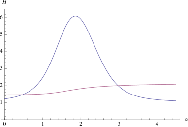
Figure 1: Upper curve: $H(\alpha)$ for the case $X=890$. The maximum $6.09697$ occurs at $\alpha=1.85815$; the minimal value $H=1$ is attained for $\alpha\to\pm\infty$. Lower curve: the right hand side of Eq. (12). The curves intersect at $\alpha_{\ast}=2.98$.

We list in Table 2 the numerical values determined for the constants in Eq. (12). The value for the microlensing optical depth $\sigma$ is the image A value from Refsdal et al (2000) from the image separation in the overall gravitational lensing.

Parameter	value
$M_{1}$	$2.7\cdot 10^{-7}M_{\odot}=0.090\ M_{\oplus}$
$M_{2}$	$2.4\cdot 10^{-4}M_{\odot}=80\ M_{\oplus}$
${\overline{M}}=\sqrt{M_{1}M_{2}}$	$8.05\cdot 10^{-6}M_{\odot}=2.7M_{\oplus}$
$X=M_{2}/M_{1}$	890
$\theta_{R}$	902 nas
$\theta_{E}({\overline{M}})$	6.5 nas
$\theta_{\rm eff}$	71.4 nas
$\sigma$	0.707
$\alpha_{\ast}$	$2.98^{+1.0}_{-0.5}$
$\langle t_{\rm ev}\rangle(\alpha_{\ast})$	11.1 day
$\langle\delta m_{\rm obs}\rangle(\alpha_{\ast})$	0.083

Table 2: Empirical values of microlensing parameters

Our power law slope $\alpha_{\ast}=2.98$ is steeper than the Salpeter value of 2.35. There is no reason to expect the two values to agree, since they are likely to be dominated by different processes in star and in primordial rogue planet formation.

5 Summary and Conclusions

With the quasar microlensing detection of a cosmologically significant fraction of the missing baryons (baryonic dark matter) now confirmed by high-cadence MACHO searches to the galactic center and to the LMC (Sumi et al, 2010, 2011), we investigate methods to permit investigation of the mass distribution function of the rogue planet population. The only theory that has predicted that the baryonic dark matter should exist as a population of rogue planets (Gibson, 1996) predicts that at time of formation their mass was $10^{-7}$ M_⊙, and that they should be found primarily in primordial Jeans clusters of approximately $6\cdot 10^{5}M_{\odot}$ (Nieuwenhuizen, Schild and Gibson, 2011). Such Jeans clusters have also been found in quasar milli-lensing at significant optical depth (Mao and Schneider, 1998). In the high-temperature and high-density universe at $z\sim 1000$, these sticky hydrogen spheres were formed by the usual void-condensation separation process and would have immediately interacted to form pairs, triples and pairs-of-pairs to eventually accumulate in an accretional cascade that quickly produced the first stars and left behind rogue planets of larger mass. Most Jeans clusters should have remained dark, but rapidly form stars when disturbed. A prediction of this theory is that all or most stars should be binaries.

We also demonstrate how the expected microlensing signal apparent in observed brightness fluctuations in quasars can be analyzed with a statistical theory devised by RS91. We find that the observed amplitudes of the microlensing fluctuations are approximately a factor 2 smaller than predicted, and that this mimics the amplitudes expected if the particles are not all of the same mass, but instead are distributed according to a mass function with slope approximately $2.98^{+1.0}_{-0.5}$, where the Salpeter slope is 2.35.

Our study thus far has been applied to the Q0957+561 A,B quasar system (the First Lens) for which a great deal of information on the luminous quasar structure has been inferred in SLR06. However this radio source quasar in the Lo-Hard spectral state is probably not optimum since its luminous inner accretion disc edge is probably finer than the High Soft radio quiet objects, which are also more common. Thus in the future we will extend our study to the several radio-quiet lensed quasars with time delay measurements and significant observed microlensing residuals.

References

- [1] Burud, I, 2000, Astrophys. J. 544, 117
- [2] Burud, I. 2002, Astron and astrophys, 391, 481
- [3] Catalano, P. 1997, Astronomy 25, 37
- [4] Colley, W. et al, 2002, ApJ, 565, 105
- [5] Colley, W. et al, 2003, ApJ, 587, 71
- [6] Colley, W. & Schild, R. 2003, ApJ, 594, 97
- [7] Gibson, C. H. 1996 Appl. Mech. Rev. 49, 299–315
- [8] Gould, A. and Miralde-Escude, J. 1997, ApJ, 483, L13
- [9] Mao, S. and Schneider, P. 1998, MNRAS, 295, 587
- [10] Minakov, A. et al, 2008, Proceedings of the International Conference “Problems in Practical Cosmology,” Ed. Y. Baryshev et al [St Petersburg: Russian Geographical Society], p. 180
- [11] Nieuwenhuizen, T. M., Gibson, C. H. & Schild, R. E. 2009 Europhys. Lett. 88, 49001,1–6
- [12] Nieuwenhuizen, Th. M., Schild, R. E., Gibson, C. H., 2011, J. Cosm. 15, 6030.
- [13] Paraficz, D. 2006, Astron. and Astrophys. 455, L1
- [14] Schild, R. E., Trichas, M., Protopapas, P. and Nieuwenhuizen, Th. M., submitted (2012).
- [15] Refsdal, S., Stabell, R., Astronomy and Astrophysics, vol. 250, no. 1, Oct. 1991, p. 62-66 (RS91)
- [16] Refsdal, S. et al, 2000, Astron. and Astrophys. 360, 10.
- [17] Schild, R. E. 1996 Astroph. J. 464, 125–130
- [18] Schild, R. E. 1999 Astroph. J. 514, 598–606
- [19] Schild, R. E. 2005, AJ, 129, 1225
- [20] Schild, R. Leiter, D. & Robertson, S. 2006, AJ, 132, 420 (SLR06)
- [21] Schild, R. E. & Vakulik, V. 2003 AJ 126, 689–695
- [22] Sumi, T. et al 2010 Astroph. J. 710, 1641–1653
- [23] Sumi, T. et al Nature, Volume 473, Issue 7347, pp. 349-352 (2011).
- [24] Vakulik, V. et al, 2007, MNRAS, 382, 819
- [25] Wyithe, S. and Loeb, A. 2002, ApJ, 577, 615.