X-ray properties of the Northern Galactic Cap sources in the 58-month Swift-BAT catalog

Abstract

We present a detailed X-ray spectral analysis of a complete sample of hard X-ray selected AGN in the Northern Galactic Cap of the 58-month Swift Burst Alert Telescope (Swift/BAT) catalog, consisting of 100 AGN with $b>50^{\circ}$. This sky area has excellent potential for further dedicated study due to a wide range of multi-wavelength data that are already available, and we propose it as a low-redshift analog to the ‘deep field’ observations of AGN at higher redshifts (e.g. CDFN/S, COSMOS, Lockman Hole). We present distributions of luminosity, absorbing column density, and other key quantities for the catalog. We use a consistent approach to fit new and archival X-ray data gathered from XMM-Newton, Swift/XRT, ASCA and Swift/BAT. We probe to deeper redshifts than the 9-month BAT catalog ($\langle z\rangle=0.043$ compared to $\langle z\rangle=0.03$ for the 9-month catalog), and uncover a broader absorbing column density distribution. The fraction of obscured ($\rm log\thinspace N_{\rm H}\geq 22$) objects in the sample is $\sim 60$%, and 43–56% of the sample exhibits ‘complex’ 0.4–10 keV spectra.

We present the properties of iron lines, soft excesses and ionized absorbers for the subset of objects with sufficient signal-to-noise ratio. We reinforce previous determinations of the X-ray Baldwin (Iwasawa-Taniguchi) effect for iron K-$\alpha$ lines. We also identify two distinct populations of sources; one in which a soft excess is well-detected and another where the soft excess is undetected, suggesting that the process responsible for producing the soft excess is not at work in all AGN. The fraction of Compton-thick sources ($\rm log\thinspace N_{\rm H}>24.15$) in our sample is $\sim 9$%. We find that ‘hidden/buried AGN’, (which may have a geometrically thick torus or emaciated scattering regions) constitute $\sim 14$% of our sample, including seven objects previously not identified as hidden. Compton reflection is found to be important in a large fraction of our sample using joint XMM-Newton+BAT fits ($\langle R\rangle=2.7\pm 0.75$), indicating light bending or extremely complex absorption. High energy cut-offs generally lie outside the BAT band ($E>200$keV) but are seen in some sources. We present the average 1–10 keV spectrum for the sample, which reproduces the 1–10 keV X-ray background slope as found for the brighter 9-month BAT AGN sample. The 2–10 keV log($N$)-log($S$) plot implies completeness down to fluxes $\sim 4$ times fainter than seen in the 9-month catalog. We emphasize the utility of this Northern Galactic Cap sample for a wide variety of future studies on AGN.

1. Introduction

Active galactic nuclei (AGN) are among the most powerful energy sources in the Universe, and their luminous output is due to accretion onto supermassive black holes (‘SMBHs’, e.g. Rees 1984). Strong emission from AGN has been observed across the entire spectrum, including at radio, sub-mm, infrared, optical and ultraviolet wavelengths, but an invaluable key to understanding them is provided by X-ray observations. X-rays are not subject to the heavy host-galaxy dilution present in other bands, and can penetrate through greater amounts of absorbing material in the line of sight than is possible with observations in other wavebands. This last feature is important in AGN studies because absorbed AGN are thought to constitute a significant proportion of the overall AGN population; it is therefore essential to have as complete a survey of AGN as possible across a range of absorbing column densities before one draws conclusions about the AGN population as whole.

While X-ray surveys of AGN are more penetrating than optical ones (e.g., Mushotzky 2004), those AGN with heavy obscuration (with neutral Hydrogen column density $N_{H}>10^{23-24}$) still can fall out of the purview of typical X-ray imaging satellites. Progressively larger amounts of absorption depress the fluxes at successively higher energies, and eventually the 0.4–10 keV, band explored by observatories such as XMM-Newton and Chandra, becomes insufficient to identify and constrain absorption levels in highly-absorbed AGN. Sensitivity at $>10$ keV is required to obtain a more complete AGN census. The Burst Alert Telescope (BAT, Barthelmy et al. 2005) on the Swift satellite has proven extremely useful for this purpose, and is producing an all-sky survey of AGN in the 14–195 keV band, the Swift/BAT catalog of AGN. The survey is augmented by detections at increasing depth as the BAT instrument continues to survey the sky. Source lists and sample properties have been presented for the catalog after the first 9 months of surveying (Tueller et al., 2008), 22 months (Tueller et al., 2010), 36 months (Ajello et al., 2009), 58 months, 60 months (Ajello et al., 2012), and the 70 month catalog source list is now in preparation.

Much work has been done on the 9-month BAT catalog (consisting of 153 sources), such as studies of their X-ray properties (Winter et al. 2009, W09 hereafter), optical properties (Winter et al., 2010), host-galaxy properties (Koss et al., 2011a) and construction the nuclear AGN spectral energy distributions (Vasudevan et al., 2009, 2010). The X-ray absorption properties of the AGN in the 36-month catalog have been presented in Burlon et al. (2011) (199 sources). This work draws from the published 58-month catalog which contains 1092 sources, of which $\sim 720$ are AGN candidates (i.e., have a counterpart identified as a galaxy, AGN, Seyfert, blazar, or BL Lac, but confirmed to not have a counterpart that is a Galactic black hole binary/neutron star/white dwarf/pulsar). As the catalog becomes increasingly sensitive, the data present a great opportunity to improve and refine the conclusions drawn from the previous versions of the catalog, in particular the detailed X-ray analysis of W09.

The numbers of AGN in the BAT catalog make it prohibitive to perform pointed observations and analysis for the X-ray properties for all $\sim 720$ AGN. The fraction of AGN with good (XMM-Newton quality, at $\gtrsim 4000$ counts) 0.4–10 keV data over the whole sky is much smaller for the 58-month sources than it is for the 9-month sources, requiring a more targeted approach. The various studies on properties of BAT AGN mentioned above have concentrated on subsamples from the BAT catalog, including a recent, very thorough X-ray spectral analysis of 48 Seyfert 1–1.5 AGN in (Winter et al., 2012). However, the sources in that paper were selected based on optical type and specifically to understand the prevalence of ionized absorbers, and therefore the average properties of the sample cannot be directly compared with the complete sample analysed in W09 as they miss heavily obscured sources by construction. Our overall goal here is to update the analysis of the complete 9-month catalog from W09 and the subsequent analysis of the 36-month catalog in Burlon et al. (2011) with a representative, unbiased subsample from the 58-month catalog. We therefore concentrate on a more manageable sample in the Northern Galactic Cap ($b>50^{\circ}$, 4830 $\rm deg^{2}$ or 1.47 steradians, 11% of the sky); the sample we focus on in this paper has almost exactly the same number of objects as W09’s uniform sample (102 objects), so we can manageably perform our analysis to a comparable level of detail as done in W09.

The aims of our study are threefold: firstly, to obtain the absorbing column density for this complete sample; secondly, to provide a detailed spectral analysis of a ‘uniform sample’ akin to the one identified in W09; and thirdly, to fit the higher quality 8-channel BAT spectra alongside 0.4–10 keV data when they provide extra information on the processes at work in these AGN, not attempted previously in the W09 analysis. We discuss the importance of each of these goals below.

Understanding the true distribution of column densities in the AGN population has been a question of particular interest in X-ray studies of AGN. Studies of the X-ray background (e.g., Gilli et al. 2007, Brandt & Hasinger 2005, Treister & Urry 2005, Worsley et al. 2005, Gandhi & Fabian 2003) suggest that the majority of accretion in the Universe must be obscured. If we wish to determine the true, intrinsic AGN power output, a knowledge of the amount of absorbing material is needed. We aim to determine the true distributions of X-ray absorption and emission properties using a complete and representative subset of the least-biased sample of local AGNs. We use the best-quality X-ray spectral data available: therefore XMM-Newton is employed preferentially if archival data are present (supplemented by 13 new XMM-Newton observations taken specifically for this study); other sources of X-ray data are detailed in §2. We determine the column density and nature of the X-ray absorption. In W09, complex X-ray absorption was found to be common ($\approx 55$%) in the 9-month catalog BAT AGNs; we produce new estimates of the covering fraction of such complex absorption where it is present. Quality measurements of the level and nature of X-ray absorption are important for deriving reliable absorption-corrected luminosities over the broadest possible X-ray bandpass; the luminosities presented here will therefore be useful in constructing low-redshift luminosity functions used to assess the amount of accretion and black-hole growth in the local universe. Our absorption measurements can also serve as a useful $z\lower 2.15277pt\hbox{$\;\buildrel<\over{\sim}\;$}0.1$ “anchor” for assessments of the dependence of X-ray absorption upon luminosity, Eddington ratio ($L/L_{\rm Edd}$), and redshift. The 0.4–10 keV spectra are fit jointly with Swift/BAT spectra from 14–195 keV to constrain absorption reliably in heavily obscured AGNs ($N_{\rm H}\lower 2.15277pt\hbox{$\;\buildrel>\over{\sim}\;$}10^{23}$ cm^-2), including those with Compton-thick X-ray absorption ($N_{\rm H}>1.4\times 10^{24}$ cm^-2).

Renewing the W09 analysis of detailed spectral features will provide further constraints on the physical processes at work in AGN. In W09, the authors search for iron K-$\alpha$ lines at or near 6.4 keV, soft excesses (spectral excesses below $\sim 1.5$ keV) and signatures of ionized absorbers or winds (edges in the spectrum). With a knowledge of the abundance of such features and any correlations present (such as the X-ray Baldwin effect linking iron line equivalent width with 2–10 keV intrinsic luminosity (e.g, Iwasawa & Taniguchi 1993), we can better understand the importance of processes such as X-ray reflection (e.g., Ross & Fabian 2005) or complex absorption (e.g., Done & Nayakshin 2007).

The 14–195 keV BAT data have improved in quality significantly since the W09 study. Only four energy channels were available in the publicly available BAT spectra for the 9-month catalog, whereas the 8-channel spectra for the 58-month catalog sources can be downloaded easily from the link provided in Footnote 1. Knowledge of the spectrum across the entire 0.4–200 keV energy range will better constrain the absorbing column density in heavily obscured objects (as done by Burlon et al. 2011) and, taking our cue from Winter et al. (2012), we also use the latest BAT spectra to constrain X-ray reflection in a subset of our sources with XMM-Newton data (extending the analysis to the absorbed sources in our sample). One problem that has plagued such analyses in the past is that the BAT spectra are averaged spectra from 58 months of monitoring, whereas the 0.4–10 keV spectra are snapshots taken for periods of typically $\sim 2-20$ ks. We therefore do not have simultaneous data across the whole X-ray band, a significant concern since the X-ray emission from AGN varies rapidly throughout the 0.4–200 keV bandpass (Beckmann et al., 2007), and the cross-normalization between the 0.4–10 keV data and the BAT data for a given observation is therefore not known. We present a strategy in this paper by which the BAT spectra can be renormalized to be quasi-simultaneous with the 0.4–10 keV observations, using the publicly available BAT light curves.

We also present an analysis of ‘hidden’ or ‘buried’ AGN as done in W09 in order to unearth examples of obscured AGNs with a small fraction of scattered nuclear X-rays (e.g., Ueda et al. 2007). These sources have small levels of scattered X-ray continuum. Such objects constitute 24% of the 9-month BAT sources in W09; they may have obscuration subtending most of the sky as seen by the X-ray source, or emaciated scattering regions.

A higher fraction of good-quality 0.4–10 keV coverage is available for our chosen sky region (augmented by an XMM-Newton proposal by PI Brandt to complete the 22-month catalog XMM-Newton coverage) than for the whole catalog. This region of the sky has high value for AGN researchers because it also has extensive multi-band imaging and spectroscopic coverage in the Sloan Digital Sky Survey (SDSS, York et al. 2000) and other surveys including WISE (IR, Wright et al. 2010), 2MASS (IR), GALEX (UV), and FIRST (radio, Becker et al. 1995), providing a ready opportunity to extend this work to construct broad-band spectral energy distributions and to understand the host-galaxy properties for a complete sample. Using the Northern Galactic Cap also ensures low Galactic absorption and more reliable source identification, due to less potential for confusion with Galactic sources. Our complete subsample is therefore optimally selected for its potential for future multi-wavelength studies.

We present this subsample as a low-redshift analog to more distant samples, such as the Chandra Deep Fields (CDFS-N/CDFS-S, e.g. Falocco et al. 2012, Lehmer et al. 2012), the COSMOS field (Brusa et al., 2007) and the Lockman Hole (Rovilos et al., 2011). The multi-wavelength work done on the deep fields has proved very illuminating for studies of AGN, and our chosen sky region has excellent potential for similar wide-ranging multi-wavelength work, as additional observational campaigns are directed at this region of the sky. The low redshifts offer the distinct advantage of better quality data for most objects; we outline in this work how we can use this sky region to understand AGN accretion comprehensively in the local universe with an unbiased sample, offering the potential to link our findings to those from the deep fields at higher redshifts.

One of the key features of this study is the systematic and uniform way in which we have analysed all of our X-ray spectra. The methods implemented in our scripts and workflows perform a wide range of useful functions on data from different X-ray detectors. All data (regardless of detector used) are fit with the same suite of models, and chi-squared comparisons are automatically performed on all of the models fit to determine the best-fit model for a particular source. If the peculiarities of a particular instrument require a different fitting approach, this can be readily extended due to the modular, object-oriented way in which the workflows have been designed. The fitting is semi-automated; i.e., models are initially fit to the data and can be inspected and modified if needed, then re-fit; but preliminary ‘first-look’ fits of large numbers of spectra for many sources can also be done in the background without user interaction. The combined properties of all sources can be readily gathered together in minutes, and the full range of properties, plots, correlations presented in this paper can be readily extended to other subsamples in the BAT catalog or indeed other catalogs. These tools can potentially be used to produce a complete, consistent X-ray analysis of the entire BAT catalog in the longer term.

In §2.1 we outline the sample and data sources used. In §3 we describe the data processing and fitting of the X-ray data in detail. In §4 we present the results from our analysis, including the absorbing column density and luminosity distributions along with analyses of features in the 0.4–10 keV data. In §5 we discuss the utility of joint 0.4–10 keV fits with the 14–195 keV BAT data. In §6 we present the average stacked spectrum for the entire sample and the log(N)-log(S) diagram to estimate the sample completeness. In §7 we compare results for the smaller 22-month catalog source list (with $90\%$ XMM-Newton coverage) with our full results for the 58-month catalog ($49\%$ XMM-Newton coverage), to 1) to identify whether the higher quality data available for the 22-month subset allows more robust determination of the sample properties, and 2) quantify any differences between the properties of this deeper sample and earlier versions of the catalog. Finally, in §8 we summarize our findings and present the conclusions. We employ the cosmology $H_{\rm 0}=71$ $\rm km\thinspace s^{-1}\thinspace Mpc^{-1}$, $\Omega_{\rm M}=0.27$ (assuming a flat Universe, i.e., $\Omega_{\rm M}+\Omega_{\rm\Lambda}=1$) throughout.

2. The Sample and the Data

2.1. Sample Definition

We employ the 58-month BAT catalog source list as presented online (Footnote 1) as the definitive source list for the whole, all-sky catalog. The catalog contains 1092 entries of which we determine 720 to be AGN candidates, with a mean redshift of $\langle z\rangle=0.16$ ($0.045$ excluding blazars and BL Lacs) providing an excellent local AGN survey for our purposes. The signal-to-noise ratio ($S/N$) is above 4.8 for all objects in the catalog list available; Tueller et al. (2010) identify that such a threshold yields 1.54 spurious detections in the entire 22-month catalog (i.e., there should be 1.54 BAT detections due to random fluctuations with $S/N>4.8$), and this number should hold good for the 58-month catalog also, yielding that the number of a false detections in our region of the sky is less than 0.5, and is therefore negligible.

We generate a potential list of targets by filtering the objects in the 58-month catalog to select only those with Galactic latitude $b>50^{\circ}$. This criterion produces a list of 143 targets in the desired region of the sky, out of which 31 are blazars, BL Lacs, flat spectrum radio quasars (as identified from NED and the BAT catalog counterpart types) and are excluded from further analysis. We also exclude 3 galaxy clusters (Coma Cluster, ABELL 1914 and ABELL 2029). Of the remaining 109 sources, 3 lack counterpart identifications at the time of writing (SWIFT J1138.9+2529, SWIFT J1158.9+4234, SWIFT J1445.6+2702), and we leave them out of the current study in the absence of a reasonable AGN/Galaxy counterpart identification in another waveband. The remaining 106 sources consist of Seyferts (Type 1 and 2 and intermediate types), quasars/AGN, LINERs, and the more general category of galaxies, including 2 ‘X-ray Bright Optically Normal Galaxies’ (XBONGs).

It is essential to have good-quality X-ray spectral data to determine the absorbing column densities accurately for these AGN, and such data in the soft X-ray regime (0.4–2 keV) are particularly important if we wish to identify any signatures of ionized absorption such as $\rm O\thinspace VII$ and $\rm O\thinspace VIII$ edges at 0.73 and 0.87 keV, or ‘soft excess’ components which often peak at $\sim$0.1–0.4 keV. At present, a large fraction of the BAT AGN in the most recent 58-month catalog do not have good-quality XMM-Newton data available in the archives. To try to obtain the true underlying $N_{\rm H}$ distribution for local AGN from a relatively complete sample, we have therefore selected an area of the sky for which obtaining XMM-Newton follow up to complete the sample is most economical (i.e., requires the fewest number of new observations to produce a complete sample). We have already discussed the advantages and detailed properties of the chosen Northern Galactic Cap region (Galactic latitude $b>50^{\circ}$, solid angle 4830 $\rm deg^{2}$) in the previous section. A successful XMM-Newton proposal by PI Brandt has extended the XMM-Newton coverage of this region with 13 new observations. As mentioned above, confusion with Galactic sources is minimized at this high Galactic latitude, and the Galactic neutral hydrogen absorbing column density is also low (0.61–4.08 $\times 10^{20}\rm cm^{-2}$).

2.2. Sources of X-ray Spectral Data

We use the XMM-Newton X-ray Science Archive (XSA) to download all the available XMM-Newton data for the 106 sources, and find that 49 of these objects have XMM-Newton spectra (including the new observations from the XMM-Newton proposal). We therefore provide as complete an analysis as possible for the 49 AGN candidates with XMM-Newton data, and turn to the Swift-X-ray Telescope (XRT) and ASCA archives to provide basic coverage for the remaining sources. The Swift/XRT is of particular utility here since the XRT has been used specifically to target BAT sources, and the BAT team routinely obtains XRT exposures to gather counterpart information on BAT detections. We prefer Swift-XRT over Chandra in this study since Chandra observations are not available as extensively for BAT sources as XRT observations are. Additionally, for sources with the typical X-ray fluxes seen in this sample, Chandra observations would usually exhibit pile-up. We downloaded XRT data for 45 of the remaining sources, and ASCA data for a further six sources. We find that five sources do not have any data available at the time of writing (LBQS 1344+0233, VCC 1759, NGC 3718, Mrk 653 and 2MASXi J1313489+365358). This constitutes a final list of 100 objects for which we have obtained data from XMM-Newton, XRT, or ASCA. The data sources used for each object are provided in Table 1.

3. Spectral Analysis

We present the distribution of total counts per observation (in the 0.4–10 keV band) obtained using different observatories in Fig. 1. We can see that the XMM-Newton data clearly have far better statistics than XRT or ASCA, but some of the XMM-Newton observations at the lower-counts end of the distribution may also not be suitable for a comprehensive analysis of spectral features. We therefore only assess the significance of iron K-$\alpha$ lines, soft excesses and warm absorber signatures for objects with $>4600$ counts in the observation used (summing over all detectors in the observatory, e.g. pn counts + mos1 counts + mos2 counts for XMM-Newton observations). This threshold allows, for example, the detection of a 100 eV equivalent width iron line over a $\Gamma=1.8$ continuum at the 3$\sigma$ level. For all remaining objects, we perform more basic fits to determine fundamental properties such as luminosity and intrinsic absorbing column density.

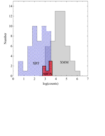
Figure 1.— Histogram of total counts (0.4–10 keV) per observation for the 100 objects in our study. XMM-Newton (49 objects) clearly shows far superior counts statistics compared to Swift-XRT (46 objects) and ASCA (6 objects).

3.1. Data Reduction

3.1.1 XMM-Newton data

The XMM-Newton data were downloaded from the XMM-Newton Science Archive (XSA) and were reduced according to the standard guidelines in the XMM-Newton User’s Manual, using the XMM-Newton Science Analysis Software (sas) version 9.0.0. The tasks epchain and emchain were used to reduce the data from the pn and MOS instruments, respectively. Initially a circular source region of radius 36^′′ was used to extract a source spectrum, checking for nearby sources in the extraction region and reducing the source region size to exclude them if needed. Background regions were either chosen to be circles near the source or annuli which exclude the central source. Additionally, the background light curves (between 10–12 keV) were inspected for flaring, and a comparison of source and background light curves in the same energy ranges was used to determine the portions of the observation in which the background was sufficiently low compared to the source; the subsequent spectra were generated from the usable portions of each observation. The sas tool epatplot was used to determine whether pile-up was present in the observations; if strong pile-up was found, we followed the recommended approach of using annular source regions to excise the piled-up core of the source, and re-calculated spectra and light curves until the strong pile-up was removed. Response matrices and auxiliary files were generated using the tools rmfgen and arfgen, and the final spectra were grouped with a minimum of 20 counts per bin using the grppha tool.

3.1.2 XRT data

We downloaded the XRT data from the High-Energy Astrophysics Science Archive (HEASARC) . Pipeline-processed ‘level 2’ FITS files were readily available from HEASARC, ready for further processing. The pipeline-processed event files from the XRT detector were processed using the XSELECT package, as directed in the Swift-XRT user guide. Source regions of 50 ^′′ were used, with larger accompanying background regions (average radius ∼150 ^′′), and care was taken to exclude other sources in source and background regions. Background light curves were determined from the event files and inspected for flaring, but this was not found to be a problem in any of our observations. Source and background spectra were extracted, and the source spectra were grouped with a minimum of 20 counts per bin by default, or a lower limit of 10 counts per bin for observations with few counts. The following objects had their spectra grouped to 10 counts per bin: 2E 1139.7+1040, 2MASX J13105723+0837387, 2MASX J13462846+1922432, B2 1204+34, CGCG 291-028, MCG -01-30-041, MCG +05-28-032, NGC 4939, NGC 5106 and Ark 347. Some objects have too few counts to construct a spectrum (NGC 4180, NGC 4500, MCG -01-33-063, CGCG 102-048 and 2MASX J13542913+1328068); for these we present basic luminosity estimates and other quantities (including upper limits where appropriate) in Appendix B.

3.1.3 ASCA data

ASCA spectra (pre-reduced) were downloaded from the Tartarus archive for the sources 3C 303.0, Was 49b, Mrk 202, NGC 4941, Mrk 477 and NGC 4619, for which Swift-XRT or XMM-Newton data were not found at the time of writing.

The details of all observations used are presented in Table 1, including their sky positions, the instruments used to provide the X-ray data, observation dates, counts in the observation and optical types. The optical types have been gathered from a variety of sources, primarily the NASA/IPAC Extragalactic Database (NED) and visual inspection of multiwavelength images and spectra; as a result these types are very heterogeneous. We do not use these types further in our analysis but provide them for completeness, and urge interested readers to check the types before using them in multi-wavelength work.

3.2. Spectral Fitting

We consistently fit a suite of models to all the 0.4–10 keV spectral data available to determine the best-fitting model in each case, using python and tcl scripting with the xspec package (Arnaud, 1996). For some XRT observations, or for XMM-Newton observations with few counts or with large portions of the observation excluded due to flaring, we impose a lower energy limit greater than 0.4 keV.

By default, we fit only the 0.4–10 keV data in order to concentrate on the accurate determination of soft X-ray feature parameters, but where the counts in the soft band ($<10\thinspace\rm keV$) are insufficient to obtain a good constraint on $N_{\rm H}$ or to analyse features (we adopt the threshold of 4600 counts for this purpose), we include the BAT data in the fit, extending beyond the W09 analysis. Inclusion of the BAT data introduces its own complications, particularly due to the variability in the BAT band over the 58 months during which the spectra were constructed; we return to these issues in §3.3 and §5. For all objects, we perform a comparison between a detailed fit in the 0.4–10 keV band and a broader, ‘continuum-only’ fit to 0.4–200 keV before arriving on a best-fit model. For objects with sufficient counts where the BAT data are not included in our final best-fit model, we perform a check to ensure that inclusion of the BAT data does not modify the spectral properties recovered from 0.4–10 keV data alone; surprisingly we find that the addition of the higher energy BAT data do not significantly alter the best-fit parameters found from analysing the lower-energy XMM-Newton results alone. In summary, we find the BAT data are only required to constrain the continuum and absorption in very high column density sources, where there are insufficient counts in the 0.4–10 keV band to constrain the soft X-ray spectral features.

All models include Galactic absorption by default (determined using the nh tool from the ftools suite of utilities, Blackburn 1995); this is by design uniformly low for this sample ($0.61<N_{\rm H}^{\rm Gal}<4.08\times 10^{20}\thinspace\rm cm^{-2}$). We follow W09 by classifying AGN spectra into two broad categories: those with ‘simple’ absorbed power-law spectra (with or without features such as an iron line at 6.4 keV, ionized absorption edges, or a soft excess below $\sim$ 2 keV); and ‘complex’ spectra for which partially covering absorbers or double power-law models must be invoked to provide a statistically acceptable fit to the spectrum. The various model sub-types are presented in Table 2. We differ slightly from W09’s analysis by not employing a model combination that includes both partial covering and a black-body component, as used for a handful of their sources; we use the term ‘soft excess’ in this work to refer uniformly to an excess above a clear power-law in which the spectrum shows low neutral absorption, and do not use the term to refer to the soft features often seen in heavily absorbed spectra, as these are probably due to different physical processes. We systematically and self-consistently fit all of the model combinations using our semi-automated system which initially fits the data with a model, presents the findings to the user allowing any necessary adjustments or re-seeding/freezing of parameters, and re-fits the data with the refined model. In this study, we also introduce the category of an ‘intermediate’ model type, where either two models fit the data equally well (e.g., $\chi^{2}/\rm d.o.f<1.0$ in both cases) or visual inspection of a fitted spectrum revealed that, whilst a partial covering model may fit the data better in a formal sense, the spectrum did not show obvious signatures of strong complexity. For this class of objects, we present the results for both models in all subsequent tables and figures and indicate them clearly. Thirteen such intermediate spectral-type objects in our sample highlight the need for better quality data (for cases where both simple or complex absorption models over-fit poorer quality data), or for further investigation of the spectra (in the cases where good-quality data reveals an indeterminate spectral shape).

Additionally, we emphasize that the complement of models used here encompasses the most common characterisations of AGN X-ray spectra, and do not represent an exhaustive list of physical scenarios. We do not attempt to model all of the more intricate features that may be present, and as a result we do see some poor fits (null hypothesis probabilities $<5\times 10^{4}$), primarily due to not modelling complex iron lines and line emission at soft energies in complex-absorption sources. These cases are briefly discussed in Appendix C.

We fit the models in Table 2 to all spectra (omitting model combinations with features such as soft excesses, iron lines, or edges for XRT or ASCA data due to lower signal-to-noise ratio or lower sensitivity below 1 keV), and determine the best-fitting model by ordering the model fits based on their reduced chi-squared values. Although we only analyze the properties of soft excesses, lines and edges for objects with $>4600$ counts, we fit models including these features to all XMM-Newton datasets and later exclude objects below the counts threshold when determining the prevalence and sample-wide properties of such features. We also estimate the significance of components such as lines, edges and soft excesses by requiring a reduction in chi-squared of 4.0 per degree of freedom for a feature to be deemed ‘significant’ (corresponding to a $\approx 95$% confidence detection of the feature). The basic fit results are presented in Table 3, and the analysis of detailed features (iron lines, soft excesses, and ionized absorber edges) is presented in Table 4. Fig 4 shows some example spectral fits, showing both the raw spectrum with the ratio of the data to the model ($\rm counts\thinspace s^{-1}\thinspace keV^{-1}$ against energy in keV in the upper panel, ratio of data-to-model against energy in keV in the lower panel) and a $\nu\thinspace F_{\nu}$ spectrum (unfolded through the response, $\rm keV^{2}\times(Photons\thinspace s^{-1}\thinspace cm^{-2}\thinspace keV^{-1})$) for 3 objects. Table 8 shows basic results for objects with very few counts, including upper limiting luminosities. In Table 4, we show upper limiting equivalent widths, soft-excess strengths and warm-absorber edge optical depths when these features produce a reduction in chi-squared, but are not significant according to the $\Delta\chi^{2}>4.0$ criterion.

We also present a plot of $\chi^{2}$ against the number of degrees of freedom ($n\rm\thinspace d.o.f$) for all the fits in our sample in Fig. 2 to illustrate the quality of the fits, as done by Mateos et al. (2010) (Fig. 2 of their paper). The solid line represents 1:1 correspondence between $\chi^{2}$ and $n\rm\thinspace d.o.f$, and the dashed lines represent the extremal values of $\chi^{2}$ above or below which we would expect less than a 1$\%$ probability of obtaining such a $\chi^{2}$ if the model is correct. We color code the objects by spectral type, with red triangles showing ‘simple’ spectral types and green squares showing ‘complex’ ones. At low $n\rm\thinspace d.o.f$ (hence low counts), almost all fits lie within these limits, but at higher $n\rm\thinspace d.o.f$, we do see some worse fits (the maximal reduced chi-sqared for the whole sample is $\chi^{2}/n\rm\thinspace d.o.f\approx 4.0$), with a majority of these objects exhibiting ‘complex’ spectral types. A comparison of our plot with Fig. 2 of Mateos et al. (2010) shows that our sample extends to higher $n\rm\thinspace d.o.f$, due to a number of datasets with greater counts than those in their study. Our plot also shows that a majority of the objects with poor fits have complex spectral types. In the high counts regime, we encounter spectra of very high quality (with high counts statistics) exhibiting strong spectral complexity that cannot be modeled by the suite of model combinations used here, including notably NGC 4151 and Mrk 766. Another notable outlier, II SZ 010, whilst having a ‘simple’ spectral type, exhibits a poor fit due to the inclusion of the BAT data in the fit, and very low flux in the BAT band at the time of the XRT observation (see §3.3). We find that removing the BAT data brings $\chi^{2}/n\thinspace\rm d.o.f$ much closer to 1.0 without altering the key results (photon index, column density) for this object.

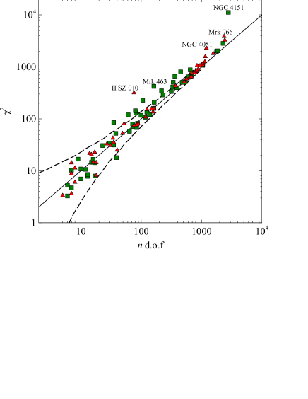
Figure 2.— Plot of $\chi^{2}$ against the number of degrees of freedom ($n\rm\thinspace d.o.f$) for the best-fit models for each source. Red triangles represent objects with ‘simple’ model spectral types, and green squares represent ‘complex’ ones (as defined in Table 2). The solid line indicates $\chi^{2}=n\rm\thinspace d.o.f$, and the dashed lines indicate the limiting $\chi^{2}$ for a given $n$  d.o.f above or below which we expect less than a 1$\%$ probability of seeing such extremal values of $\chi^{2}$ if the model is correct (see Mateos et al. 2010).

We present the rest-frame 2–10 keV observed luminosity (not corrected for absorption) against redshift in Fig. 3, to characterize the redshift distribution of the sample. All sources are located at redshifts $z<0.2$, with an average of $\langle z\rangle=0.043$, slightly higher than the average of 0.03 obtained in both W09 for the 9-month BAT catalog and in Burlon et al. (2011) for the 36-month catalog.

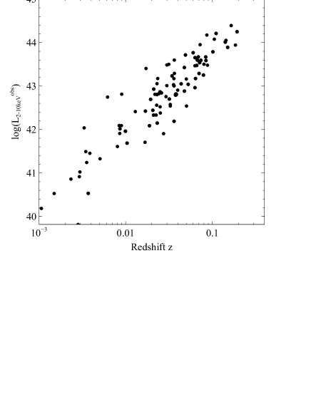
Figure 3.— Observed 2–10 keV luminosity $L_{\rm 2-10keV}^{(obs)}$ (not corrected for absorption) against redshift for the 100 sources in our sample.

Figure 4.— Some example spectra from our sample, with the left panel plots showing the spectrum and ratio plot, and the right panel plots showing the $\nu F_{\nu}$ plots. The objects are, from top-to-bottom, NGC 5899 (XMM-Newton data), NGC 5290 (XRT+BAT data) and 3C 303.0 (ASCA data).

3.3. On the issue of simultaneity across the entire 0.4–200 keV band

The BAT spectra have been gathered over the entire duration of the survey, and are therefore not in any sense ‘simultaneous’ with the 0.4–10.0 keV data used from XMM-Newton, Swift/XRT or ASCA. It is important to use simultaneous observations wherever possible when combining multi-wavelength data due to the variable nature of AGNs. This is even more pertinent at high energies, where the short-time scale variability is reflective of rapidly changing accretion processes occurring close to the inner regions of the accretion flow.

Whilst we cannot obtain a BAT spectrum simultaneous with the 0.4–10 keV observation due to insufficient counts in the BAT instrument in such short ($1-100\rm ks$) time intervals, we can attempt to account for this effect in some measure using the BAT light curves. These are available for each BAT catalog source, spanning the entire 58 months of the survey. The variability displayed for the BAT AGN in these light curves indicates that the true 14–195 keV spectrum at a particular epoch within the survey may look significantly different to the final averaged 58-month spectrum. Such variation will be composed of two components: variation in the overall normalization (i.e., flux) and spectral shape. We aim to account for the former effect in this work. Variability in spectral shape requires particularly good signal-to-noise ratio to paramaterize properly, and a full treatment of this effect will be presented in Shimizu et al. (in prep.). Their preliminary analysis of hardness ratios for the brightest $\sim 30$ BAT sources reveals minimal spectral variability across 14–195 keV, but this analysis is only possible on the brightest sources on variability timescales greater than 30 days. Ideally we prefer truly simultaneous data (such as will be obtained with co-ordinated NuSTAR and 0.4–10 keV campaigns, or ASTROSAT) alongside the 0.4–10 keV data to be able to interpret the broad-band spectral shape fully.

Many of our soft (0.4–10 keV) X-ray observations have been taken within the timeframe of the BAT survey. Where possible, the BAT light curve is used to estimate the variation in the overall normalization of the BAT spectrum, by considering the BAT flux ratio relative to the full 58-month average, at the date of observation of the soft X-ray data.

We then re-normalize the BAT spectrum accordingly, whenever the soft X-ray data have been taken within the span of the BAT survey. We show an example in Fig. 5. The key improvement in this approach is produced when fitting the XMM-Newton/XRT/ASCA spectra jointly with the BAT data within xspec: without such renormalization, we would have to allow the normalizations of the XMM-Newton/XRT/ASCA and BAT data to ‘float’ with respect to each other because of this uncertainty in the absolute normalization of the BAT spectrum due to non-simultaneity with the 0.4–10 keV data. However, by re-normalizing, we can lock the normalizations of the BAT and 0.4–10 keV (XMM-Newton/XRT/ASCA) components together, removing a degree of freedom from the fit and providing more stringent constraints on the parameters obtained from model fits. This is particularly useful when performing fits to determine reflection parameters, which we will return to in §5.2.

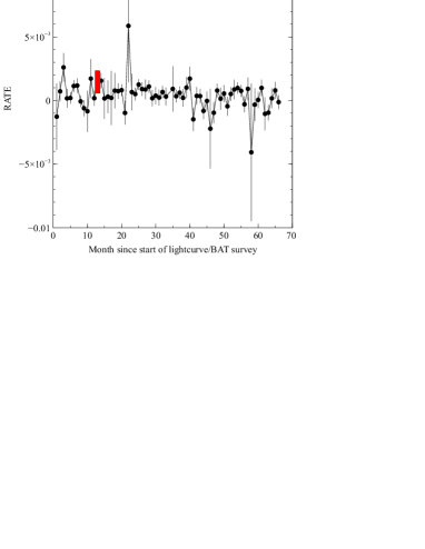
Figure 5.— Illustration of the renormalization of the BAT spectrum using the light curve for Mrk 1310. The top panel shows the BAT light curve, with a red bar indicating the date of observation of the 0.4–10 keV data. The 0.4–10 keV data are from XRT in this case. The middle panel shows the 58-month averaged BAT spectrum used as-is along with XRT data, whereas the bottom panel shows the renormalized BAT spectrum (thereby made ‘quasi-simultaneous’ with the XRT data). Prior to re-normalization, the spectrum looks like a continuous unabsorbed power-law across 0.4–200 keV, but after re-normalization, the spectrum has the appearance of strong reflection or complex absorption.

The utility of this renormalisation is illustrated in Fig. 6, where we plot the 2–10 keV flux against the BAT (14–195 keV) flux, color-coding the observations based on the measured column density from spectral fitting. We overplot lines showing the expected ratio of $F_{\rm 2-10keV}/F_{\rm 14-195keV}$ for different fiducial absorption levels and intrinsic photon indices, to indicate the predicted locus of objects in this plot depending on absorption and spectral slope. In the left panel we see that before re-normalization, the fluxes cluster tightly close to the BAT flux limit for our sample, irrespective of absorption and do not lie in the regions expected for their measured column density. After re-normalization (right panel of Fig. 6), the objects overwhelmingly shift into the expected regions for the three fiducial column density ranges shown.

There is one outlier in the far left of the right panel of Fig. 6, the low-absorption source 2MASX J12055599+4959561 for which the re-normalization does not appear to work well. When re-normalization is applied, this object lies far from the expected position in $F_{\rm 2-10keV}-F_{\rm 14-195keV}$. This behaviour is contrary to expectations, since we would expect that re-normalizing the BAT data to be contemporaneous with the 2–10 keV data would improve the congruence between the two luminositites. This object also displays an unusual ratio of $L_{\rm 14-195keV}$/$L_{\rm 2-10keV}$ (Fig. 7). Inspection of the joint XRT+BAT spectrum reveals a renormalized BAT spectrum that lies below the XRT spectrum in flux. If we use the raw BAT spectrum without re-normalization, the BAT and XRT spectra link continuously in a $\nu F_{\nu}$ plot, with a hard, simple power-law spectrum with $\Gamma=1.5$ and negligible $N_{\rm H}^{\rm intrinsic}$. Inspection of the BAT light curve shows that there is a pronounced dip at the time the XRT data were taken, and that the source is very faint in the BAT band. This might imply that the re-normalization occasionally fails for very faint sources, but for all other objects the re-normalization produces results consistent with the lines of constant $\Gamma$ and $N_{\rm H}$ in Fig. 6.

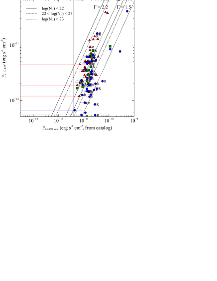
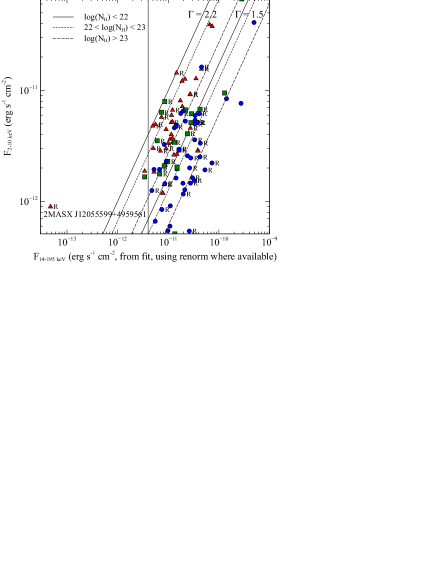
Figure 6.— Observed 2–10 keV flux ($F_{\rm 2-10keV}$) against BAT flux ($F_{\rm 14-195keV}$). The red triangles represent sources with $N_{\rm H}<10^{22}\rm\thinspace cm^{-2}$, while the green circles represent sources with $N_{\rm H}>10^{23}\rm\thinspace cm^{-2}$. Blue squares indicate the intermediate column sources. Sources for which renormalization of the BAT data was done are indicated using an ‘R’. The left panel shows the comparison if the BAT flux is calculated from the average spectra presented in the 58-month catalog, and the right panel shows the results obtained if we re-normalize the BAT spectrum as detailed in §3.2 . The vertical line indicates the flux limit of our sample based on the average fluxes reported in the 58-month catalog.

4. Results

4.1. Average Sample Properties and Distributions

The average BAT luminosity for our sample is $\langle\rm log(L_{\rm 14-195keV})\rangle=43.5,\sigma_{L_{\rm 14-195keV}}=1.1$. This result is similar to the average BAT luminosity of $\langle\rm log(L_{\rm 14-195keV})\rangle=43.7,\sigma_{L_{\rm 14-195keV}}=0.8$ from the 9-month catalog (using W09’s results), and for consistency, we exclude any objects with jets analyzed in W09 in calculating this average. We also present plots of the BAT-X-ray colors/hardness ratios as done in W09 for easy comparison of our present, deeper sample to the 9-month catalog results. In Fig. 7 we see the soft color $F_{\rm 0.5-2keV}/F_{\rm 2-10keV}$ plotted against the hard color $F_{\rm 14-195keV}/F_{\rm 2-10keV}$. The range of colors spanned in the 58-month catalog appears larger on both axes than that seen in W09. In the same region of parameter space spanned by the 9-month catalog, we see the same division into regimes occupied by high, intermediate, and low absorption sources, but there are three sources with extreme values (outside the range of the plot): these are 2MASX J12055599+4959561 (for which $\rm log\thinspace N_{\rm H}\thinspace<22$, $F_{\rm 14-195keV}/F_{\rm 2-10keV}<0.1$, and $F_{\rm 0.5-2keV}/F_{\rm 2-10keV}\approx 0.4$), 2MASX J13105723+0837387 and CGCG 291$-$028 ($\rm log\thinspace N_{\rm H}\thinspace>23$, $F_{\rm 14-195keV}/F_{\rm 2-10keV}\approx 10$, and $F_{\rm 0.5-2keV}/F_{\rm 2-10keV}<10^{-5}$). For CGCG 291$-$028 and 2MASX J13105723+0837387, the model fits have very little 0.5–2 keV flux, but this is likely due to their poor XRT data quality, since these objects required the inclusion of BAT data to obtain a fit at all. For 2MASX J12055599+4959561, the highly unusual ratio of BAT flux to 2–10 keV flux indicates a renormalized BAT spectrum that lies below the XRT spectrum in flux, due to a dip in the BAT light curve at that date, as discussed in §3.3.

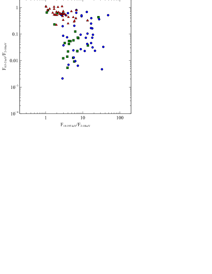
Figure 7.— The 58-month BAT AGNs with $b>50^{\circ}$ with soft and hard fluxes plotted on the color-color plot initially presented in Winter et al. (2008), and later in W09. The red triangles represent sources with $N_{\rm H}<10^{22}\rm\thinspace cm^{-2}$, while the circles represent sources with $N_{\rm H}>10^{23}\rm\thinspace cm^{-2}$. Squares indicate the intermediate column sources.

W09 presented the diagnostic plot $L^{\rm intrinsic}_{\rm 2-10keV}/L_{\rm 14-195keV}$ versus $L^{\rm intrinsic}_{\rm 2-10keV}+L_{\rm 14-195keV}$, showing the regions of the plot populated by objects of different photon indices $\Gamma$; we reproduce this plot in Fig. 8. We note the unusual location of 2MASX J12055599+4959561 again as in Fig. 7, and additionally highlight NGC 5683, identified as a Seyfert 1. The measured photon index for NGC 5683 is 2.15, but this source does not have a re-normalized BAT spectrum. As a result, the ratio of the measured BAT luminosity to the 2–10 keV luminosity places it in the region expected for extremely hard sources with $\Gamma<1.0$.

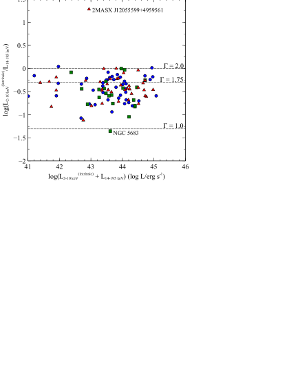
Figure 8.— Right: ratio of $L^{\rm intrinsic}_{\rm 2–10keV}/L_{\rm 14-195keV}$ vs. the total luminosity in the 2–10 keV and 14–195 keV bands. The dotted lines show values of constant $\Gamma$ between both bands at constant ratios of $L^{(}\rm intrinsic)_{\rm 2–10keV}/L_{\rm 14-195keV}$, following the presentation in W09. The different absorption levels are distinguished using the same key as in Fig. 7

We now present the distributions of key quantities including the absorbing column density (Fig. 10), photon index $\Gamma$ (Figs. 16,17,18) and 2–10 keV intrinsic luminosity (Figs. 19,20).

4.2. Radio loudness

We present the radio loudness values for our sample (defined as $\rm\nu L_{\nu}(\nu=\rm 5\thinspace GHz)/L^{\rm int}_{\rm 2-10keV}$, Terashima & Wilson 2003) plotted against the intrinsic 2–10 keV luminosity in Fig. 9, to provide an indication of the radio properties of the sample. The radio luminosities are taken from the FIRST survey at 1.4 GHz, and we convert the fluxes to 5 GHz using a standard spectral index of $\alpha=0.7$ typical for synchrotron emission (for flux density $f_{\nu}\thinspace\propto\thinspace\nu^{-\alpha}$; see e.g., Meléndez et al. 2010 for a discussion of radio spectral indices). Where no match is found within 5 ^′′ for a given source, we assume a flux limit of 0.75 mJy for the survey and use it to calculate an upper limiting radio luminosity. The large angular size of the FIRST beam is likely to introduce significant contamination from the host galaxy, but our main purpose here is to catch significant outliers where the nuclear radio emission is heavily boosted by a jet. Such objects will easily stand out from the rest of the distribution.

All of our sources have radio-loudness values below $-2$, and all but two of our sources are below the values typically seen for strongly-beamed sources such as BL Lacs or flat-spectrum radio quasars (Terashima & Wilson, 2003). The two objects with the highest radio-loudness parameters are Mrk 463 and 3C 303.0. The object 3C 303.0 is expected to be radio loud based on its inclusion in the 3C catalog. Further investigation of Mrk 463 reveals that it contains two nuclei at very close separation (3.8 kpc, Bianchi et al. 2008), with the eastern source Mrk 463E dominating the X-ray emission by a factor of $\sim 4$. The brighter Mrk 463E nucleus was previously found to have a Seyfert 2-type optical spectrum, but a fuller consideration of the radio morphology reveals that it is a ‘hidden’ Seyfert 1 nucleus (Kukula et al., 1999). Both nuclei show moderate-to-weak radio emission (Drake et al. 2003). Our XMM-Newton and Swift/BAT analysis of this source therefore is likely to include the combined emission from both sources (as discussed in Bianchi et al. 2008). We discuss these two cases in Appendix A, but a more detailed study of the X-ray properties of these objects is needed.

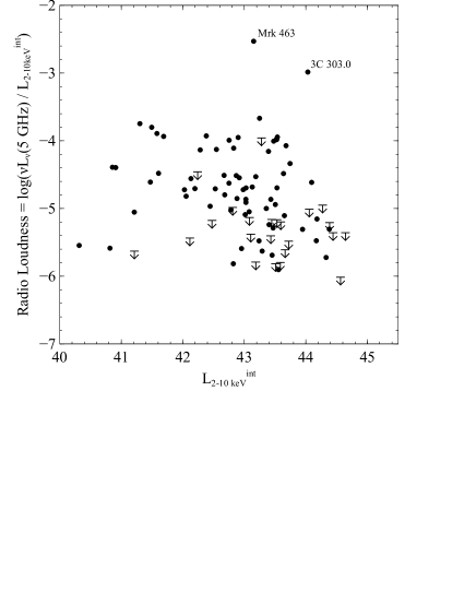
Figure 9.— Radio-loudness ($\rm\nu L_{\nu}(\nu=5GHz)/L_{2-10keV}$) against intrinsic 2–10 keV luminosity. Downward pointing arrows show upper limits where FIRST radio detections were not available (assuming a flux limit of 0.75 mJy to calculate the luminosities).

4.3. Column density $N_{\rm H}$

As the BAT survey increases its exposure, we expect it to uncover a more accurate reflection of the true absorption distribution for the AGN population, and to see differences from the earlier 9-month catalog analysis. If we compare the absorption distribution seen here (Fig. 10) with that seen in the 9-month catalog (W09, see Fig. 25 of this paper), we indeed see that our distribution shows a tail at higher column densities than that seen previously, and the average absorbing columns from our distribution are $\langle\rm log\thinspace N_{\rm H}\thinspace\rangle=20.80$, $\sigma=1.18$ (simple, 51 objects) and $\langle\rm log\thinspace N_{\rm H}\thinspace\rangle=23.55$, $\sigma=0.71$ (complex, 44 objects), assuming the ‘simple’ model type for any objects with dual best-fits. We assume all objects with $\rm log(N_{\rm H})<20$ to have a lower-limiting absorption of $\rm log(N_{\rm H})=20$ for a consistent comparison with W09. If we assume dual objects are by default complex, we find slightly different distributions: $\langle\rm log\thinspace N_{\rm H}\thinspace\rangle=20.67$, $\sigma=1.12$ (simple, 38 objects) and $\langle\rm log\thinspace N_{\rm H}\thinspace\rangle=23.27$, $\sigma=0.95$ (complex, 57 objects). We contrast these results with those from W09, who find $\langle\rm log\thinspace N_{\rm H}\thinspace\rangle=20.58$, $\sigma=0.74$ (simple, 46 objects) and $\langle\rm log\thinspace N_{\rm H}\thinspace\rangle=23.03$, $\sigma=0.71$ (complex, 56 objects), verifying a tail of higher-absorption objects in our sample. If we split the objects based on the spectral complexity exhibited, we find that the percentage of ‘complex’ objects is in the range 43–56% (of the whole sample, 100 objects), with the range again due to the presence of sources with ambiguous spectral types. However, inspection of Fig. 11 shows that the absorption distributions reported in our sample do not vary appreciably depending on BAT flux. Interestingly, in the region of flux space already covered by the 9-month catalog, we find an increase in the average absorbing column density towards the highest BAT fluxes.

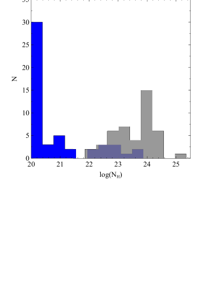
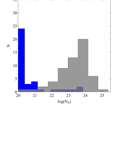
Figure 10.— Histograms of absorbing column density $\rm log(N_{\rm H})$. The blue shaded portions represent simple spectrum objects, whereas the semi-transparent grey shaded portions represent complex spectrum objects (semi-transparent to show the underlying blue histogram when present). In the left panel, any objects with ambiguous spectral classifications (both a simple and a complex spectral model describe the data well) have been assumed to be simple spectrum objects; in the right panel those same objects are assumed to possess complex spectra.

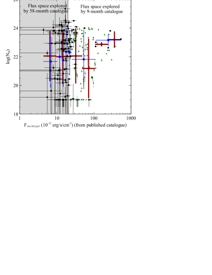
Figure 11.— Absorbing column density log($N_{\rm H}/\rm cm^{-2}$) against BAT flux ($F_{\rm 14-195~{}keV}$); black points show the results for the 58-month catalog $b>50^{\circ}$ sources and the small green triangles show the results from the 9-month catalog (from W09). The blue (thin) and brown (thick) error bars and points show the results binned by $F_{\rm~{}14-195keV}$ from two different approaches; 1) using a constant number of objects in each bin, or 2) using a constant interval in $F_{\rm 14-195keV}$ for each bin. The mean $N_{\rm H}/\rm cm^{-2}$ in each bin is calculated, and the error bars are the standard deviation to show the degree of spread (not the error on the mean). The distribution of absorption probed in this region of the sky appears to be independent of BAT flux, with a wide range of absorbing columns seen at all flux levels. We note the different distribution found in W09 and discuss this in the text.

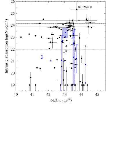
Figure 12.— Absorbing column density log($N_{\rm H}/\rm cm^{-2}$) against intrinsic 2–10 keV luminosity $L_{\rm 2-10keV}$ (absorption-corrected). The black circles represent objects for which a unique best-fit model was determined. For objects where a unique best-fit model could not be determined and two ‘best-fit’ models were identified, blue shaded areas represent the range in log($N_{\rm H}$) and $L_{\rm 2-10keV}$ spanned by those two models (with the model fit results themselves signified by blue crosses), and the blue oval points represent the central, average values for that object. The dashed horizontal line shows the conventional threshold between ‘absorbed’ and ‘unabsorbed’ objects ($\rm log\thinspace N_{\rm H}\thinspace=22$), and the dot-dashed line shows the threshold for Compton-thick objects ($\rm log\thinspace N_{\rm H}\thinspace=24.15$). All objects for which $N_{\rm H}$ was below $10^{19}\rm cm^{-2}$ are shown at log($N_{\rm H}$)=19; in these sources absorption by neutral gas has negligible effect on the X-ray spectrum.

We also identify the proportion of Compton-thick ($N_{\rm H}>1.4\times 10^{24}\rm\thinspace cm^{-2}$) sources in our sample. In contrast to W09 who find no Compton-thick objects by this criterion, we find eight Compton-thick sources in our sample: these are NGC 4102, 2MASX J10523297+1036205, 2MASX J11491868-0416512, B2 1204+34, MCG -01-30-041, MRK 1310, PG 1138+222 and UGC 05881; additionally, NGC 4941 and NGC 5106 are very close to the threshold for being Compton-thick, and the errors on their column densities could push them over the threshold. This result suggests that $\sim 9$% of our sample is Compton-thick. However, at such high column densities, basic photoelectric absorption is not sufficient to model the level of absorption present and more sophisticated absorption models must be used to calculate the column density for such objects. This exercise is beyond the scope of this paper, but we discuss alternate measures of Compton-thickness in §5.1.

The histograms in Fig. 10 show a clear bifurcation between spectral types in terms of their absorption. Simple spectra overwhelmingly fit objects with low absorption, and complex spectra are generally required for objects with high absorption. However, the intermediate class of objects identified in this study introduces some uncertainty in the distributions, since for these objects the different model types yield different estimates of $N_{\rm H}$. We therefore show the ‘worst-case’ scenarios in Fig. 10, assuming that the intermediate objects are all simple or complex in the left and right panels, respectively. Assuming that these objects take the $N_{\rm H}$ values of their complex model fits, we see a more pronounced peak in high-absorption sources. We also note that a substantial fraction of sources have negligible intrinsic absorption ($\rm log\thinspace N_{\rm H}\thinspace<20$).

The relationship between absorption and intrinsic 2–10 keV luminosity is given in Fig. 12. This plot shows a broad absorption distribution at all luminosity levels. The thirteen sources with ambiguous spectral types can have highly uncertain column densities (indicated by the blue shaded boxes). We plot the absorbed fractions (using thresholds of $\rm log\thinspace N_{\rm H}\thinspace=22$ and $23$ to defined ‘absorbed’) as a function of 2–10 keV luminosity in Fig. 13, using 10 objects per bin to determine the absorbed fraction. We do not see as strong a decrease in the absorbed fraction with luminosity as previously reported in Fig. 13 of Burlon et al. (2011) and the earlier INTEGRAL AGN survey (Beckmann et al., 2009), although a similar trend is present. Our work reveals a more homogenous distribution of absorption throughout luminosity space, and notably three heavily absorbed sources ($\rm log\thinspace N_{\rm H}\thinspace>23.5$) are found at the highest luminosities (3C 234, 2E 1139.7+1040 and 2MASX J11491868-0416512). The Burlon et al. (2011) and (Beckmann et al., 2009) samples contain more sources at high luminosities than our sample, and it is above luminosities of $10^{44}\thinspace\rm erg\thinspace s^{-1}$ where the decrement in the absorbed fraction is more pronounced. It is therefore possible that we do not have enough sources at high luminosities to see the decrement.

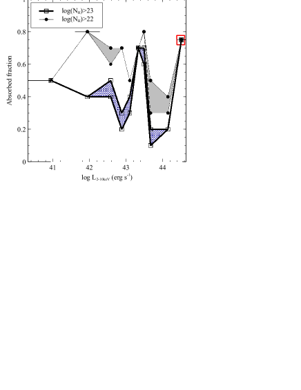
Figure 13.— Absorbed fractions against intrinsic 2–10 keV luminosity (10 objects per bin). Filled circles connected by thin solid lines show the fraction of sources with $\rm log(N_{\rm H})>22$, whereas empty squares connected by thick lines show the fraction of sources with $\rm log(N_{\rm H})>23$. The solid grey and blue hatched shading reveal the uncertainty in these fractions due to the thirteen sources with ambiguous spectral types (and hence two estimates for their $\rm log\thinspace N_{\rm H}$). The absorbed fraction in the highest luminosity bin (indicated by the red square) is more uncertain since it contains only four objects.

We see from Fig. 13 how the distribution of absorbed sources depends on the threshold absorption used; we quantify this effect in Fig. 14 by employing three thresholds of $\rm log(N_{\rm H})=(22,22.5,23)$, and plotting the fraction of objects above these thresholds against the threshold itself. We present a comparison with the 9-month catalog results. The shaded area in the figure again shows the uncertainty due to the non-unique model fits for 13 sources. It is clear that the absorbed fractions are uniformly higher at all thresholds in our work than in W09, and that the slower fall-off with absorption threshold indicates that a substantial proportion of our absorbed sources are heavily absorbed ($\rm log\thinspace N_{\rm H}\thinspace>23$), about 10% more than in the 9-month catalog. Inspection of a plot of absorbing column density against redshift (which we omit for brevity) indicates no evolution of the absorption distribution with redshift over the redshift range probed by this survey. Therefore, the deeper flux limit must be responsible for picking up more asborbed objects. At $\rm log(N_{\rm H})=23.5$, $\sim 5$% of the intrinsic flux in the BAT band is absorbed, so we would expect that the deepening of the survey would produce this kind of increase in the proportion of highly-absorbed objects.

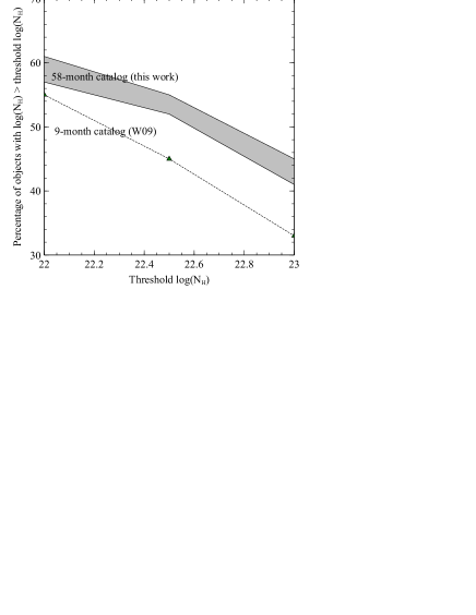
Figure 14.— Absorbed fraction vs. threshold $\rm log(N_{\rm H})$, for the 9-month catalog (W09, green triangles and dashed line) and for the 58-month catalog Northern Galactic Cap sources (solid lines and shaded area, this work). The shaded area shows the uncertainty in the absorbed fractions in this work due to the sources with ambiguous spectral types and non-unique best-fitting column densities.

4.4. Photon Index

We restrict photon indices to lie between $1.5<\Gamma<2.2$ in our fits for observational and physical reasons: observationally, the AGN in the XMM-Newton Bright Serendipitous Survey (Corral et al., 2011) indicate 3$\sigma$ limits on their absorption-corrected photon indices consistent with this restriction; physically, photon indices much lower (harder) than 1.5 indicate unphysical Compton $y$ parameters in standard inverse-Compton scattering scenarios for modelling the X-ray power-law emission from the corona (e.g., Zdziarski et al. 1990). Fig. 15 is a plot of $\Gamma$ against the intrinsic X-ray luminosity $L_{\rm 2-10keV}$, and the distribution of photon indices as histograms is presented in Figs. 16 and 17.

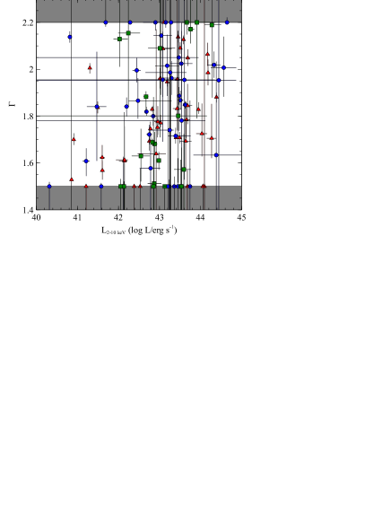
Figure 15.— Photon index $\Gamma$ against intrinsic (absorption-corrected) 2–10 keV luminosity $L_{\rm 2-10keV}$. The grey shaded areas delineate the hard limits imposed on $\Gamma$ in the fit. Red triangles depict low absorption ($\rm log\thinspace N_{\rm H}\thinspace<22$) objects, blue circles depict high absorption objects ($\rm log\thinspace N_{\rm H}\thinspace>22$) and green squares represent objects with intermediate absorptions between these two limits.

Earlier studies have investigated whether photon index is correlated with luminosity or Eddington ratio; larger photon indices (softer X-ray spectra) are seen to accompany higher accretion rates with more prominent accretion disc components in Galactic Black Hole candidates, constraining the physics of different accretion states (for a review see e.g., Remillard & McClintock 2006). This parallel has also been explored with AGN (e.g., Körding et al. 2006, Shemmer et al. 2008). Fig. 15 shows that there is no observed correlation between photon index and 2–10 keV luminosity, although the more physically relevant correlation is with Eddington ratio, which we do not explore here as we lack black hole mass estimates for the entire sample. The limits imposed on $\Gamma$ could prevent us from seeing any correlation, if present; however, if the range $1.5<\Gamma<2.2$ is an appropriate physical constraint to place on $\Gamma$, then this should not be an issue. In any case, our study reinforces the result in W09 that the photon index does not appear to be correlated with 2–10 keV luminosity, at least in our complete sample of objects, although W09 suggest that they may be correlated when comparing multiple observations of an individual object. We also note that for the high-absorption sources, the photon index is more prone to uncertainty due to complex absorption, and that the photon indices in such sources are more likely to serve simply as an indication of the general spectral shape. If we therefore restrict our view to unabsorbed, $\rm log(N_{\rm H})<22$, sources in our search for a correlation between $\Gamma$ and $L_{\rm 2-10keV}$, we still do not observe any obvious correlation, but note that there is a larger range of $\Gamma$ values at high luminosities, whereas low $L_{\rm 2-10~{}keV}$ luminosities seem to accompany lower values of $\Gamma$. We defer further investigation of this topic to a dedicated study on multi-epoch observations of BAT sources.

We find that in high-absorption objects, the photon index hits our hard limits imposed on $\Gamma$ more frequently. In objects with $\rm log(N_{\rm H})>22$, we see a larger fraction of objects with pegged extremal (1.5 or 2.2) spectral indices (20/60, 33%) compared to low-absorption $\rm log(N_{\rm H})<22$ objects (7/40, 18%), indicating that the spectral complexity due to higher absorption ultimately needs a more sophisticated modelling approach.

We present histograms of the photon index in Figs. 16, 17 and 18. Low-absorption sources appear to peak at $\Gamma\approx 1.8$ ($\langle\Gamma_{\rm lowabs}\rangle=1.81$, $\sigma^{\rm(lowabs)}_{\Gamma}=0.21$), whereas high-absorption sources show a wider spread in $\Gamma$ and often hit the hard limits imposed ($\langle\Gamma_{\rm highabs}\rangle=1.84$, $\sigma^{\rm(highabs)}_{\Gamma}=0.26$). Complex sources appear to have a wide range of photon indices ($\langle\Gamma_{\rm complex}\rangle=1.87$, $\sigma^{\rm(complex)}_{\Gamma}=0.25$), but hit the $\Gamma=2.2$ boundary more often than simple model sources ($\langle\Gamma_{\rm simple}\rangle=1.79$, $\sigma^{\rm(simple)}_{\Gamma}=0.22$) which, as expected, show a peak at around $\Gamma\approx 1.8$ (since they overwhelmingly overlap with low-absorption sources). Due to the large error bars on some values of photon indices, we present histograms of the values of $\Gamma$ with absolute errors less than 0.05 in Fig. 18, and find that these trends are borne out even when restricting ourselves to the well-determined values of photon index. High-absorption objects with well-determined $\Gamma$ values show a distribution skewed toward slightly higher values of $\Gamma$ ($\langle\Gamma_{\rm highabs}\rangle=1.90$, $\sigma^{\rm(highabs)}_{\Gamma}=0.28$) than found above, as do complex objects ($\langle\Gamma_{\rm complex}\rangle=1.90$, $\sigma^{\rm(complex)}_{\Gamma}=0.28$), but simple spectrum or low-absorption objects with well-determined photon indices do not show significant differences in their distributions, when comparing with the whole sample of simple/low-absorption objects. The uncertainties in the fits for the thirteen ambiguous spectral-type objects do not affect these statistics by more than 0.02 for any of the quantities presented.

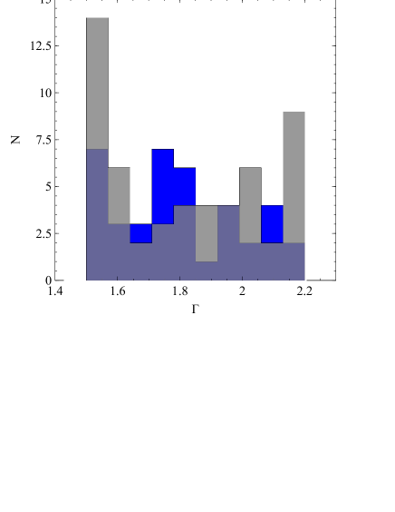
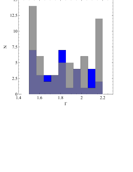
Figure 16.— Histograms of 2–10 keV photon index, $\Gamma$. The grey shaded portions represent high-absorption objects ($\rm log\thinspace N_{\rm H}\thinspace>22$), whereas the blue shaded portions represent low-absorption objects ($\rm log\thinspace N_{\rm H}\thinspace<22$). In the left panel, in order to split our objects into the two absorption categories, any objects with ambiguous spectral classifications and two ‘best-fit’ $N_{\rm H}$ estimates (both a simple and a complex spectral model describe the data well) have been assumed to have the smaller of the two $N_{\rm H}$ estimates. In the right panel, the maximal $N_{\rm H}$ is assumed for objects with ambiguous spectral classification.

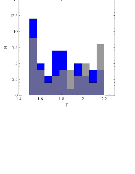
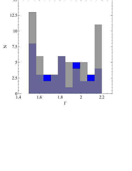
Figure 17.— Histograms of 2–10 keV photon index, $\Gamma$. The grey shaded portions represent complex spectrum objects, whereas the blue shaded portions represent simple spectrum objects. In the left panel, in order to split our objects into the two spectral-type categories, any objects with ambiguous spectral classifications (both a simple and a complex spectral model describe the data well) have been assumed to be simple spectrum objects; in the right panel those same objects are assumed to possess complex spectra.

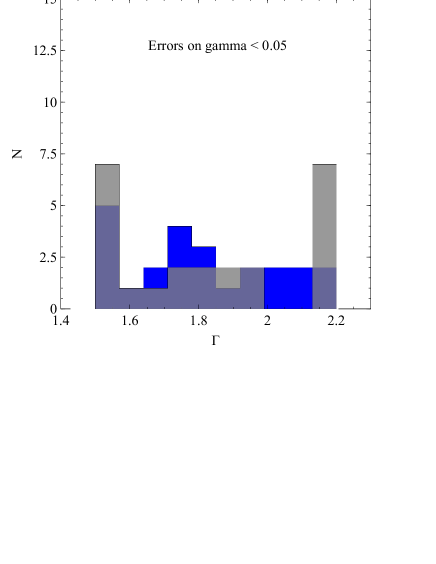
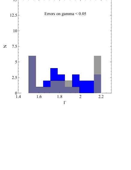
Figure 18.— Histograms of 2–10 keV photon index, $\Gamma$, with objects with large errors on $\Gamma$ removed. The grey shaded portions represent complex spectrum objects, whereas the blue shaded portions represent simple spectrum objects. In the left panel, the grey shading represents high absorption objects and blue shading represents low absorption (dividing line between these designations is $N_{\rm H}=10^{23}\rm cm^{-2}$ as before). The right panel shows the same values split on model type, such that grey represents complex spectrum objects and blue represents simple spectrum objects. For objects with dual spectral classifications, we assume simple spectral types and the smaller of the two $N_{\rm H}$ estimates.

4.5. 2–10 keV intrinsic luminosity

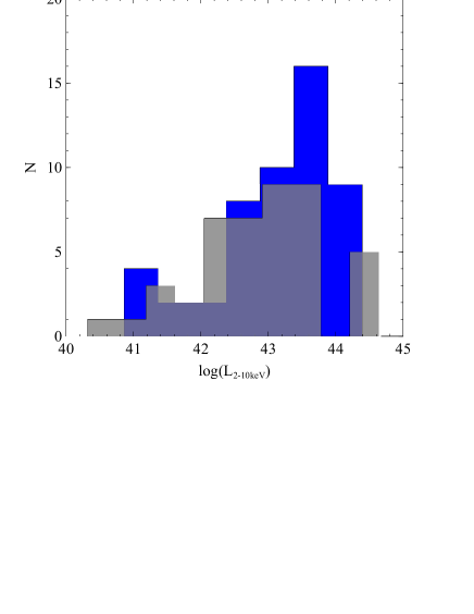
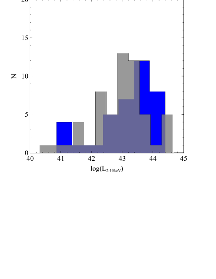
Figure 19.— Histograms of intrinsic 2–10 keV luminosity log($L_{\rm 2-10keV}$). The grey shaded portions represent complex spectrum objects, whereas the blue shaded portions represent simple spectrum objects. In the left panel, any objects with ambiguous spectral classifications (both a simple and a complex spectral model describe the data well) have been assumed to be simple spectrum objects; in the right panel those same objects are assumed to possess complex spectra.

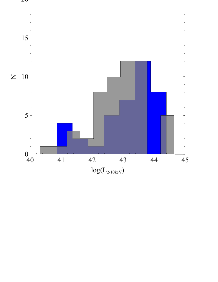
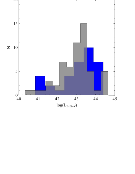
Figure 20.— Histograms of intrinsic 2–10 keV luminosity log($L_{\rm 2-10keV}$). The grey shaded portions represent high-absorption objects ($\rm log\thinspace N_{\rm H}\thinspace>22$), whereas the blue shaded portions represent low-absorption objects ($\rm log\thinspace N_{\rm H}\thinspace<22$). In the left panel, any objects with ambiguous spectral classifications and two ‘best-fit’ $N_{\rm H}$ estimates (both a simple and a complex spectral model describe the data well) have been assumed to have the smaller of the two $N_{\rm H}$ estimates. In the right panel, the maximal $N_{\rm H}$ is assumed for objects with ambiguous spectral classification.

The average 2–10 keV luminosity for the sample is $\langle\rm log(L_{\rm 2-10keV}/\rm erg\thinspace s^{-1})\rangle=43.00$, with $\sigma_{\rm logL}=0.91-0.92$, similar to the distribution seen in W09 ($\langle\rm log(L^{\rm 9month}_{\rm 2-10keV}/\rm erg\thinspace s^{-1})\rangle=43.02$, with $\sigma_{\rm logL}=0.87$), but we notice differences when we split the sample based on the absorption level or spectral complexity. Inspecting the histograms in Figs 19 and 20 shows that complex/high-absorption sources appear to have a wider distribution in luminosity than simple/low-absorption sources, notably showing more of a spread to low luminosities. Indeed, Fig. 12 demonstrates this broader distribution of absorbed sources. The simple/complex bifurcation again closely corresponds to the low/high absorption split. Simple/low absorption objects have an average luminosity of $\rm log(L_{\rm 2-10keV})=43.02-43.11$, with $\sigma_{\rm logL}=0.87-0.98$ (the ranges take into account the uncertainty in spectral type for some sources). For complex/absorbed sources, we find a slightly lower average $\rm log(L_{\rm 2-10keV})=42.88-42.97$, $\sigma_{\rm logL}=0.89-0.96$.

4.6. Hidden/Buried Sources

This class of sources was identified as a potentially important component of the X-ray background in Ueda et al. (2007), and the proportion of such AGN in the BAT catalog has been discussed in Winter et al. (2008) and W09; the latter find that $\approx 24$% of the 9-month BAT AGN are hidden. The criteria employed to define such hidden AGN are that the model is complex (best fit by a partial-covering model) with a covering fraction $f\geq 0.97$ and a ratio of soft (0.5–2 keV) to hard (2–10 keV) flux $\leq 0.04$. A partial covering fraction greater than 0.97 implies a scattering fraction below 3% and is suggestive of a geometrically thick torus or an emaciated scattering region. We identify a total of 13-14 hidden/buried sources in our sample using these criteria. Of these, two were previously identified as hidden sources in W09 (CGCG 041-020 and SWIFT J1309.2+1139 - NGC 4992), one narrowly missed identification as a hidden source in W09 (Mrk 417, using the same data), three were analysed in W09 but did not pass the criteria for being deemed hidden (NGC 4138, NGC 4388 and NGC 4395), and the remainder are newly identifed hidden objects (KUG 1208+386, Mrk 198, NGC 5899, NGC 4258, NGC 4686, Mrk 268, NGC 4939 and MCG +05-28-032). For NGC 4138, we again use the same data as analyzed in W09, but the best-fit adopted by W09 is taken from the Cappi et al. (2006) study. Cappi et al. fit NGC 4138 with a power-law plus soft-excess model, whereas our systematic model comparisons reveal that a partial covering model is clearly preferred over a soft-excess model for this particular observation.

We point out that in this work, a uniform model-fit-comparison approach has been adopted for all objects, unlike W09, where some model fits were taken from the literature; for consistency, we perform all our analysis on the results from our own fits. For NGC 4388, we have used XMM-Newton data in our study, whereas ASCA data were used previously in W09 where it narrowly escaped classification as ‘hidden’; we prefer our analysis of the better-quality XMM-Newton data for defining the hidden status of this object. The ‘hidden’ classification of NGC 4395 can be called into question since it exhibits rapid variability (e.g., Vaughan et al. 2005), which may argue for a reflection interpretation instead of the complex absorption seen here; we present its reflection properties in §5.2 where we are only able to produce an upper limit on the reflection parameter ($R<0.71$). Further detailed study of this source is needed. MCG +05-28-032 has only XRT data and is of an intermediate model type; close inspection reveals that the covering fraction is not well determined and has a large error due to poor quality data, so it may not be hidden.

Our finding of 13–14 hidden sources indicates a percentage of hidden sources of $\approx 14$%, lower than the 24% fraction found in W09. However, if we assume Poissonian errors on the counts used to calculate these percentages, the proportions of hidden objects in the two samples are consistent to within $2\sigma$. We emphasize that we have adopted a uniform strategy for fitting models to all of our data, whereas in W09 many fits were gathered from the literature. This difference may partly explain the differing proportion of hidden sources identified. The identification of seven new hidden objects (three with newly obtained XMM-Newton data) is nevertheless interesting. The average absorption for these hidden sources is $\rm log(N_{\rm H})=23.42$ with $\sigma_{\rm logN_{\rm H}}=0.44$, and their average soft-to-hard flux ratio is $F_{\rm 0.5-2keV}/F_{2-10keV}=0.02$ with $\sigma=0.01$, consistent with the W09 results for hidden objects.

4.7. Detailed Features

We present the fraction of objects for which soft excesses, iron lines, and warm absorber edges are well detected, for the subset of objects with at least 4600 counts in the observation (39 objects). The data sets are all from XMM-Newton, and the properties of these features are detailed in Table 4 below. We are careful to calculate upper limiting parameters for these components in all cases where fitting does not reveal a significant improvement to the fit; this approach allows a more complete analysis of properties later.

4.7.1 Iron K-$\alpha$ lines

We find that 79% of the objects with $>4600$ counts exhibit iron lines, which is very close to the 81% found in W09. For the remaining sources, we include a zgauss model fixed at an energy of 6.4 keV with a width of $\sigma=0.1$ keV and fit the normalization. We obtain the upper limiting equivalent width by setting the normalization to its upper limiting value as determined in xspec, and determining the equivalent width using the eqwidth command.

From Fig. 21 (left panel), we see that there are suggestions of an anti-correlation between the iron line equivalent width and 2–10 keV absorption-corrected luminosity, known as the ‘X-ray Baldwin Effect’ (Iwasawa & Taniguchi, 1993). However, the presence of many upper limiting equivalent widths complicates this picture. Since the upper limiting equivalent widths occupy the same range as those for well-detected iron lines, we use the asurv (Astronomy Survival Analysis) package for censored data (from the STATCODES suite of utilities; Feigelson & Nelson 1985) to determine the correlation parameters. We obtain a very shallow anti-correlation of $\rm log(EW/\rm keV)=(3.678\pm 2.406)-(0.104\pm 0.056)\times\rm log(L_{\rm 2-10keV})$ with a Spearman’s Rank coefficient of $-0.275$ (Spearman probability 0.078). We use the E-M algorithm whenever results from asurv are presented; the alternative Buckley-James algorithm yields very similar results with slightly steeper slopes. However, the definition of the equivalent width requires a good knowledge of the intrinsic continuum over which the line is detected; significant or complex absorption in many sources may make it difficult to recover the ‘true’ iron line equivalent width in those cases. Therefore, we also check the presence of an anti-correlation for the 24 sources with $\rm log(N_{\rm H})<22$. We find a slightly steeper relation, $\rm log(EW/\rm keV)=(5.41\pm 3.14)-(0.14\pm 0.07)\times\rm log(L_{\rm 2-10keV})$ with a Spearman’s Rank coefficient of $-0.356$ (Spearman probability 0.088). These results are consistent with the Page et al. (2004) finding and later works by Jiang et al. (2006) and Bianchi et al. (2007) for radio-quiet AGN.

We inspect the residuals of all of the XMM-Newton fits for hints of broad iron lines that can indicate the presence of strong-gravitational processes at work in the inner part of the accretion flow near the black hole. A systematic analysis of such lines in our sample is not presented here, but we identify four sources with XMM-Newton data that display hints of complex iron lines by inspection of residuals, but have too few counts ($<4600$) to fit an iron line successfully (Mrk 417, UGC 06527, NGC 4686 and SWIFT J1309.2+1139), two sources that definitely exhibit structure in the lines beyond what is shown here using our simple zgauss fits (Mrk 766 and NGC 4051), and five sources that show possible signs of broad lines by inspection of residuals (NGC 5252, NGC 5273, UM 614, NGC 4151, NGC 4579). Many of the more well-known sources have been analysed in more detail (e.g., Nandra et al. 2007, Cappi et al. 2006), and in other works on individual sources.

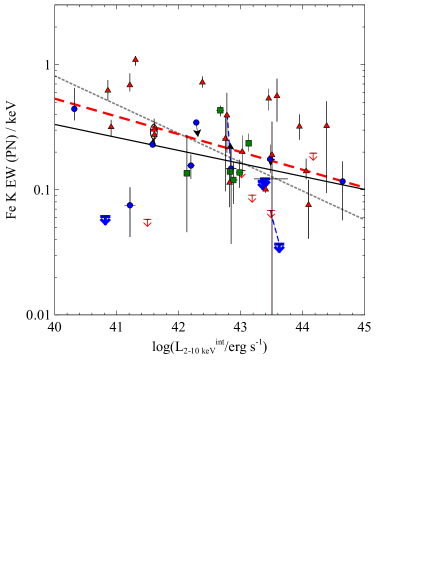
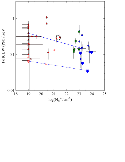
Figure 21.— Left panel: iron line equivalent width from the PN instrument (for objects with $>4600$ counts in all detectors) vs. $L_{\rm 2-10keV}$ (absorption-corrected). Downward pointing arrows with horizontal lines show upper limiting iron line equivalent widths wherever a source did not have a statistically significant iron line (using the zgauss model). Triangles (red) show $\rm log(N_{\rm H})<22$ sources, circles (blue) show $\rm log(N_{\rm H})>23$ sources, and squares (green) show the remaining sources with intermediate absorbing columns. Right panel: iron line equivalent width (PN) against absorbing column density; the symbols and color-coding are the same as for the left panel. Absorbing columns below $10^{19}\thinspace\rm cm^{-2}$ are shown at $N_{\rm H}=10^{19}\thinspace\rm cm^{-2}$. In both figures, dashed lines or ellipses connect two different measurements for an individual source when a unique best-fit model was not found. The black thin solid line shows a best-fit (including upper limits using asurv) using all objects; the red dashed line shows the fit to only unabsorbed ($\rm log\thinspace N_{\rm H}\thinspace<22$) objects. The grey dotted line shows the anti-correlation found in W09, using binned data.

4.7.2 Soft excesses

Many X-ray spectra of low-absorption AGN reveal an excess at energies below $\sim$1 keV. A number of possible origins have been suggested for this soft excess: blurred reflection (e.g., Ross & Fabian 2005), complex absorption (e.g., Sobolewska & Done 2007) or an extension of thermal emission from the accretion disc, possibly more visible in low black hole mass AGN (e.g. Narrow Line Seyfert 1 AGN). A definitive physical picture has not yet emerged to explain the soft excess in all AGN; we therefore employ a simple redshifted black body component (e.g., Crummy et al. 2006) as a phenomenological description of the feature, and we do not attempt to fit the more complex models described above to the soft excess. An inventory of the observed properties of the soft excesses in our sample will allow future investigations into their physical origins. We find that 31–33% of the objects with $>4600$ counts in their spectra have soft excesses (with the range due to ambiguous spectral types for a few sources), compared to 41% in W09 (consistent within Poisson errors). All of the objects for which soft excesses are detected have intrinsic absorbing column densities $\rm log(N_{\rm H})<21.22$, so we restrict ourselves explicitly to soft excesses seen above ‘unabsorbed, simple power-law’ type spectra as mentioned in §3.2.

We define the ‘soft-excess strength’ $S_{\rm softex}$ as the ratio of the luminosity in the black body component only (setting the power-law normalization to zero, integrating the luminosity from 0.4 to 3 keV) to the luminosity in the power-law component only (setting the black body normalization to zero), measured between 1.5 and 6 keV ($S_{\rm softex}=L_{\rm BB}/L^{\rm(PL)}_{1.5-6keV}$); these energy ranges were selected so we could be confident of avoiding features such as edges and iron lines. This approach is an extension of the concept presented in W09 where the power present in the soft excess was compared to that seen in the power-law component, but here we adopt the fractional measure since in some reprocessing models, we expect some fraction of the coronal power-law emission to be responsible for the soft excess. We also extend the previous analysis by producing upper-limiting soft-excess strengths for those objects where soft excesses are not detected, and show the soft-excess strength against power-law luminosity in Fig. 22. The upper limits are calculated by including a black body component with a temperature fixed at the canonical soft-excess temperature 0.1 keV (e.g., as found in the sample of Crummy et al. 2006 or Gierliński & Done 2004), finding the upper limiting normalization, thereby determining the upper limiting black body luminosity. Amongst the objects with detected soft excesses, we see a small decrease in soft-excess strength with higher power-law luminosities (in constrast to the simple proportionality seen in W09 between soft excess luminosity and power-law luminosity), but there are too few points at low luminosities to be able to constrain the slope of any such trend. This result may suggest that a straightforward reprocessing scenario, where the power in the power-law component (due to the corona) is somehow recycled in the soft excess, is not favored. However, this hypothesis would be better tested on a larger sample of objects.

The remainder of the objects (for which upper limits have been calculated) occupy a completely different part of parameter space than those with detected soft excesses. The objects with upper-limiting soft-excess strengths span a range of luminosities and lie well below the anti-correlation between $S_{\rm softex}$ and $L_{\rm 1.5-6~{}keV}$ for the objects with detected soft excesses. This disjoint distribution suggests that there are two classes of objects: those which show measurable, statistically significant soft excesses, in which there is a weak anti-correlation between soft-excess strength and luminosity, and those without any detectable soft excess, in which the stringent upper limits on the soft-excess strength dictate that there can be little scope for any kind of correlation or anticorrelation in those sources. This dichotomy suggests that the physical process responsible for the soft excess occurs in some AGN only, and that a soft excess is not an intrinsic part of all AGN spectra. We return to this issue in a companion paper on the relation between reflection/absorption and soft-excess strength in our sample (see §5.2).

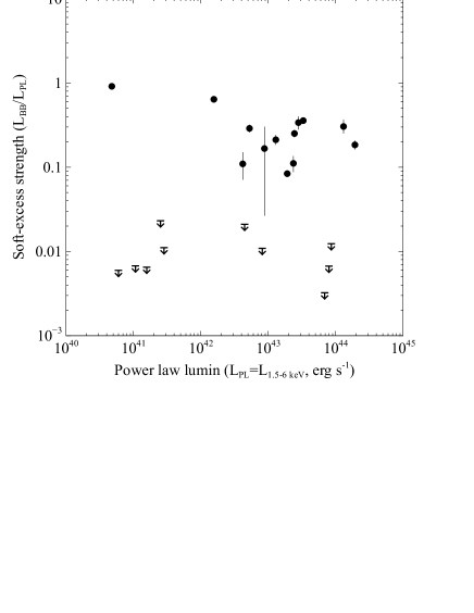
Figure 22.— Soft-excess strength against power-law luminosity ($L_{\rm 1.5-6keV}$). The soft excess is modelled as a black body, and its strength is parameterized as the ratio of the luminosity in the black body component only to the luminosity in the power law between 1.5 and 6 keV (determined from the PN instrument). Downward pointing arrows show upper limiting soft-excess strengths wherever a source did not have a statistically significant soft excess (using the zbbody model).

We also want to ensure that the stronger soft excesses are not biased to being found in sources with harder spectra ($\Gamma<2.0$): a harder spectrum leaves more scope for soft features to be seen as an excess. We see from Fig. 23 that this is not the case; for the two objects with the largest soft-excess strengths (NGC 4051 and Mrk 766, which also happen to show pronounced spectral variability) we do indeed see that they have hard ($\Gamma=1.5$) spectra, but for all other objects, the opposite trend seems to be evident, i.e., the strength of the soft excess increases with $\Gamma$ (as the spectrum gets softer), in line with the trend previously found in Brandt et al. (1997).

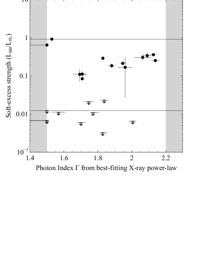
Figure 23.— Soft-excess strength against photon index $\Gamma$. The soft-excess strength is parameterized as described in Fig. 22. Downward pointing arrows show upper limiting soft-excess strengths wherever a source did not have a statistically significant soft excess (using the zbbody model).

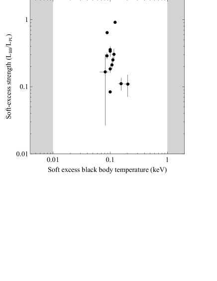
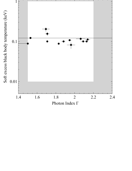
Figure 24.— Left: soft-excess strength against soft excess temperature (using the black body model as a parameterization for the soft excess). The soft excess temperatures are clustered at $\sim 0.1$ keV, as found in previous works. Right: soft excess black body temperature against photon index $\Gamma$.

We lastly investigate whether there is any relation between the temperature of the soft excess and the soft-excess strength or $\Gamma$. In line with what has been found previously (e.g., W09, Crummy et al. 2006, Gierliński & Done 2004), we find a narrow distribution of temperatures ($\langle kT_{\rm softex}\rangle=0.113,\sigma_{\rm kT}=0.032$) and can identify no discernible correlation with either soft-excess strength or photon index. This result lends credence to the idea that the soft excess is not part of the direct, thermal accretion disk emission since the temperature at which it is seen is uniformly and tightly clustered around $\sim 0.1\rm keV$.

4.7.3 Ionized absorber edges

We present the edge depths due to ionized absorbers in Table 4. Winter et al. (2011) noted that X-ray observations do not offer the same sensitivity for picking up warm absorbers that, for example, UV spectroscopy does (such as COS spectra used in Winter et al. 2011). However, the detection rates and properties here can at least serve as an indicator of what is detected in X-rays using an unbiased sample and can be compared with UV studies. We find that 18% of our high-counts subsample show warm absorber signatures in the form of an $\rm OVII$ edge at 0.73 keV. Only 8% exhibit a significant additional warm absorber edge at 0.87 keV. However, this is measured as a fraction of all sources with $>4600$ counts; if we instead only consider the 21–23 unabsorbed ($\rm log\thinspace N_{\rm H}\thinspace<22$) sources within this high-counts subset, we find that the fraction of such sources with at least one well-detected ionized absorber edge rises to $\sim 32\%$ (two sources with ambiguous $N_{\rm H}$ values introduce an uncertainty of $\pm 1\%$ to this figure). The study of Seyfert 1-1.5 BAT-selected AGN presented in Winter et al. (2012) reveals that $53\%$ of their 48 sources exhibit a detectable ionized absorber edge using XMM-Newton and Suzaku X-ray data; the pioneering work of Reynolds (1997) finds similarly that $50\%$ of their sources exhibit such edges in ASCA spectra, and the work of Crenshaw et al. (1999) using UV spectroscopy from HST reveals that $47\%$ of their sources show evidence for such absorbers. The latter two studies are not, however, from an unbiased sample, so we emphasize the utility of Winter et al. (2012) and this work on BAT-selected AGN. Considering the small sample sizes involved in all the above studies, our finding that $\sim 32\%$ of unabsorbed sources have measurable ionized absorption is broadly consistent with previous findings.

The sources that do exhibit well-detected warm absorbers are clustered around luminosities of $L_{\rm 2-10keV}=10^{43.8}\thinspace\rm erg\thinspace s^{-1}$, with only two sources having luminosites above $10^{44}\thinspace\rm erg\thinspace s^{-1}$. The upper limiting optical depths of the $\rm OVII$ edge for the remaining sources show increasingly stringent upper limits that indicate less scope for ionized absorption at higher luminosities. This is consistent with a general picture where absorption of any kind (neutral or ionized) is less prevalent at high intrinsic luminosities (e.g., Winter et al. 2012 and §4.3 of this work).

4.8. New XMM-Newton observations

Our sample of 100 objects in this study includes 13 objects with new XMM-Newton observations, gathered specifically for improving the coverage of the BAT catalog at $b>50^{\circ}$. We highlight some of the interesting features of these 13 objects here. Two of these XMM-Newton datasets have been studied in more detail in other works already: Mrk 817 (Winter et al. 2011, a multi-wavelength study including UV spectroscopy from the Cosmic Origins Spectrograph - COS along with HST and IUE archival data, looking for outflows and broad-band variability in this source) and NGC 3758 (also known as Mrk 739, Koss et al. 2011b, identifying a faint counterpart Mrk 739W using high spatial resolution Chandra data thereby identifying a dual AGN in this system). The remaining new XMM-Newton datasets reveal diverse properties for these 13 objects (including three hidden AGN, KUG 1208+386, Mrk 198, NGC 5899 and one Compton-thick candidate NGC 4102). One object of particular note is Mrk 50, a very bright unabsorbed Seyfert 1 galaxy with a soft excess but no measurable Iron line; this object would benefit from further detailed study.

5. Including the BAT data

5.1. Compton-thick sources

Using our simple ztbabs model to model absorption, we identify eight Compton-thick sources ($N_{\rm H}>1.4\times 10^{24}\rm cm^{-2}$): NGC 4102, 2MASX J10523297+1036205, 2MASX J11491868-0416512, B2 1204+34, MCG -01-30-041, MRK 1310, PG 1138+222 and UGC 05881; NGC 4941 and NGC 5106 may be Compton thick within the errors on their fitted column densities. This constitutes $\sim 9\%$ of our sample; this is a notable change from W09 (where no Compton thick sources are detected by this definition) and Burlon et al. (2011) where 4.6% of their sample (the 36-month BAT catalog AGN) are Compton thick. However, we have not taken into account the effect of Compton scattering for our heavily absorbed sources; more sophisticated models such as plcabs or MyTorus (Murphy & Yaqoob, 2009) or that presented by Brightman & Nandra (2011) are required to model these effects. Burlon et al. (2011) examine the effect of using MyTorus for a fraction of their sources and also use the built-in xspec model cabs to take Compton scattering into account. MyTorus and similar models are sufficiently complex to warrant a separate study since they have many more parameters than simple absorption models, and determining these parameters individually for each object is beyond the scope of this study. However, a number of other measures have also been used to identify Compton-thick sources, such as a high Fe-K$\alpha$ line equivalent width, a flat photon index (here we take this to mean $\Gamma$ pegs at the minimal value of 1.5) or an unusually high reflection fraction ($R>1$) (see W09 and Table 5 for reflection values). Using these alternative metrics, W09 note that the proportion of Compton-thick AGN in the 9-month catalog could increase to 6%, although they do not use BAT data to constrain absorption in the highly absorbed sources. We employ these metrics with our sample and include our full 0.4–200 keV band fits and find that a few more sources may be Compton-thick: Mrk 766, NGC 4051, UM 614, Mrk 744, NGC 3227, CGCG 041-020. We caution that we can only use the Fe-K$\alpha$ equivalent width metric on the objects with XMM-Newton data since XRT data are not of sufficient quality to analyse these line properties, and in this study we restrict ourselves to reflection fits to objects with XMM-Newton data. The object Mrk 766 exhibits all three of these alternative signatures despite having a low column density ($\rm log\thinspace N_{\rm H}\thinspace<21$). Mrk 766 is known to be highly variable and has been extensively studied in the literature (e.g., Turner et al. 2007, where the pronounced variation in spectral shape between epochs is shown); this conclusion also holds for NGC 4051 which exhibits both a broad Iron line and a high reflection fraction, alongside well-studied variability favouring the reflection scenario (Ponti et al., 2006). There are four sources with both high reflection and $\Gamma=1.5$ (UM 614, Mrk 744, NGC 3227 and CGCG 041-020), the last three of which have absorptions at or above log($N_{\rm H}$)=23; they may also be good Compton-thick candidates. The object B2 1204+34, which only has XRT data, also exhibits $\Gamma=1.5$ reinforcing its status as Compton-thick. Based on these considerations, we may add 2–6 sources to the existing list of $\sim 9$ with measurably Compton-thick column densities, to yield a Compton-thick fraction of 11-15%. However, what is ultimately required is the use of models that fully include Compton scattering and all the possible types of reflection, coupled with an understanding of the geometry in each source, to determine the true Compton-thick fraction.

In Fig. 25, we show how the log$(\rm N_{\rm H})$ distributions vary between the 9-month (W09) and 58-month ($b>50$) catalog subsamples. We present these distributions as a fraction of the total number of objects in each sample for easy comparison. As before, we allow for the uncertainty in $N_{\rm H}$ for some sources by assuming any sources with ambiguous spectral types have the ‘simple’ absorption fit in the left panel and the ‘complex’ (partial covering) absorption fit in the right panel. The distributions for the earlier catalog and the 58-month catalog are consistent within errors (calculated according to the Gehrels 1986 Poisson approximation) for all columns up to $\rm log(N_{\rm H})\approx 23.6$; the bin centered on $\rm log(N_{\rm H})\approx 24$ shows a twofold increase in objects in the 58-month catalog, and a discrepancy remains even when errors are taken into account. Our 58-month catalog does show some objects at even higher columns, but the numbers are small. In general, these results show how the increased sensitivity of the 58-month catalog allows detection of intrinsically bright objects with $\rm log(N_{\rm H})\gtrsim 23.6$. As discussed in Burlon et al. (2011), the increased proportion of highly absorbed sources as the BAT catalog deepens in exposure suggests that the BAT hard X-ray survey is still missing a significant fraction of $\rm log(N_{\rm H})>24$ sources. We constructed simple simulations to estimate the fraction of such missed sources at higher columns, by assuming a given underlying (intrinsic) BAT flux and $N_{\rm H}$ distribution and using the ‘attenuation’ factors for the BAT flux for different column densities (ratios for the observed-to-intrinsic BAT fluxes calculated using the MyTorus model). We attempt to recover the observed absorption distribution for different flux limits corresponding to the 9-month, 58-month, and future, deeper surveys. However, we discover that the precise degree of improvement expected with deepening exposure is difficult to predict and relies on a realistic source input BAT flux distribution. We defer publishing of this simulation to a future study.

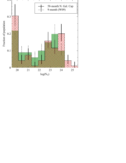
Figure 25.— Comparison of log($N_{\rm H}$) distributions between the 58-month catalog (red diagonal cross-hatching shading, solid error bars) and the 9-month catalog (solid green shading, dotted error bars). The left panel shows the 58-month column density distribution assuming that any ambiguous spectral-type objects have the ‘simpler’ model, and the right shows the results assuming that such objects are better represented by their ‘complex’ (partial-covering absorption) model fit.

5.2. Reflection

The hard X-ray BAT data provide an opportunity to constrain the reflection properties of the sample, since the Compton reflection hump peaks in the BAT band. We present the reflection properties for the subset of objects with XMM-Newton data. We fit a pexrav model to the combined XMM-Newton and BAT data, again renormalizing the BAT spectrum wherever possible (and linking BAT and PN normalizations). In our pexrav fits, we allow the reflection fraction $R$, the photon index $\Gamma$, the folding energy $E_{\rm fold}$ and the normalization to vary, fix the redshift of the source and freeze all other parameters (abundance of elements heavier than Helium relative to solar abundances, iron abundance and cosine of the inclination angle) at their default values. We ignore any data below 1.5 keV to avoid soft excesses or edges and ignore data between 5.5 and 7.5 keV to avoid the iron line and edge which are not modelled by pexrav. We include either a simple absorption component or a partial covering absorber, depending on whether the basic fit from Table 3 indicates that the 0.4–10 keV spectral shape is simple or complex, respectively. For complex objects, we seed the absorbing column density with the value of $N_{\rm H}$ obtained from our 0.4–10 keV fits. We do not impose any restriction on $\Gamma$ as done before in the power-law fits, since we wish to use $\Gamma$ here purely to constrain the spectral shape, and can then more easily probe any correlations between the different reflection parameters. For objects where the error calculation on $R$, $E_{\rm fold}$ or $\Gamma$ fails, we perform a detailed contour-plot using the steppar command in xspec to better constrain the parameters. We present the results in Table 5 and show plots of the three key variables in the reflection scenario, $R$, $\Gamma$ and $E_{\rm fold}$ in Figs. 26, 27 and 28.

We find that reflection can be constrained in a large fraction of our sources, and that for the majority of the sample, some level of reflection is required ($R>0$). The average value of the reflection parameter for the sample is $\langle R\rangle=2.7\pm 0.75$, indicating that reflection is important in this unbiased sample of AGN, in both absorbed and unabsorbed objects. This large average value indicates that strong reflection involving light bending may be common ($R>1$) or that highly complex absorption could be important. In our dataset, there are no ‘strong’ reflection ($R>4$) sources with sufficient signal-to-noise ratio (when considering the combined XMM-Newton and BAT data) to distinguish these two possibilities. However, the soft excess has been linked to reflection (e.g., Ross & Fabian 2005), and in a companion study we aim to explore how a comparison between the soft-excess strength and the reflection parameter may allow determination of which of the two scenarios, reflection or absorption, is favored in individual objects. Inspection of Fig. 26 reveals that absorbed objects (blue filled circles) exhibit similar ranges in reflection parameter as less absorbed sources. The average fold energy is well above the maximum energy of BAT, indicating that we cannot reliably detect high-energy cut-offs using BAT data alone. There is significant uncertainty in determining $E_{\rm fold}$, since when the fit yields a value outside the BAT band, we typically see very large error bars on the fit value. In Table 5, we have shown objects with $E_{\rm fold}>5000$ keV (arbitrarily chosen) as lower limits, using their negative error bar to determine the lower limit in $E_{\rm fold}$. For some objects with fold energies below 5000 keV, the positive error bar on $E_{\rm fold}$ is difficult to constrain due to the poor sampling in the BAT band. For those objects, we do not plot a positive error bar but note that the fold energy is difficult to determine in those cases. The average photon index from pexrav for the whole sample is 1.80 with a standard deviation of 0.32; the 1$\sigma$ range in photon indices falls within within the limits we previously imposed when performing our 0.4–10 keV fits. There is no evidence of any correlations between any of the three parameters $R$, $E_{\rm fold}$ and $\Gamma$ (see Figs. 27, 28). Given the limited signal-to-noise ratio and bandpass of the BAT data, one finds that one cannot separately constrain the three components of the pexrav model using BAT data alone, and that degeneracies exist between these three parameters. However, inclusion of the 0.4–10 keV data constrains the fit better, and the BAT re-normalization removes one free parameter and provides better constraints on fit parameters in many cases. Overall, our reflection fits show that reflection is present in some form in the majority of our sample. The fold energy is generally outside the BAT range and we only observe a few definitive high-energy cut-offs in our BAT data. Our determinations of $R$ and $E_{\rm fold}$ are given more credence by using the 0.4–10 keV to help lock down the overall broad-band X-ray spectral shape (via the photon index $\Gamma$).

We also briefly contrast our results with those of Winter et al. (2012), who fit a reflection model to a sample of Seyfert 1-1.5 AGN using a slightly different approach (fitting a model combination tbabs(ztbabs(cutoffpl + zbbody + zgauss + pexrav)) in xspec) to simultaneously model the soft excess, iron line, power-law, absorption and reflection, with edges added where needed). For the 8 objects that are common between our sample and theirs, they employ Suzaku data alongside BAT data and fit them with the above model combination. All of the common objects were therefore observed at different epochs in Winter et al. (2012) than presented here. We note that some objects exhibit very similar reflection fractions in the two studies (e.g., NGC 4151, NGC 4593, NGC 5548, Mrk 841) but some objects display large discrepancies (e.g., NGC 4051, Mrk 766). This could be in part be attributed to re-normalization employed here providing new constraints on the fit, but also due to intrinsic changes in the spectrum between observations. NGC 4051 and Mrk 766 in particular are known for their strong variability in both spectral shape and intensity (see §5.1 above), which is capable of producing such pronounced spectral changes.

Another interesting comparison can be made with the Ricci et al. (2011) analysis of INTEGRAL AGN detected in the 15–1000 keV band by the observatory’s soft $\gamma$-ray imager instrument. Their work differs from ours in that they use only hard X-ray spectra ($>10$ keV) to calculate reflection parameters, whereas we restrict ourselves to the subset of objects with XMM-Newton data below 10 keV to provide an additional constraint on reflection parameters. Additionally,the BAT survey is flux-limited and taken across the whole sky, unlike the INTEGRAL survey which consists of pointed observations of sources of interest. The 165 Seyfert galaxies in the INTEGRAL sample show a very similar average photon index of $\Gamma\approx 1.8$ and an unobservable average hard X-ray cut-off ($E_{\rm C}\gtrsim 200$ keV). They also show a range of reflection values, and in particular find that moderately-obscured Seyfert 2 nuclei (with $23<\rm log\thinspace N_{\rm H}\thinspace<24$) have a higher reflection component than other classes of AGN, with $\langle R\rangle=2.2^{+4.5}_{-1.1}$ for this class of sources. We do not notice any such trend in our sample and find a broad distribution of reflection amplitudes at every $\rm log\thinspace N_{\rm H}$ level, but our XMM-Newton+BAT sample is significantly smaller than theirs (49 AGN vs. 165 AGN) and we therefore may not have sufficient statistics to make a detailed comparison. We defer more detailed discussion of this issue to a companion paper on the stacked spectrum of the Northern Galactic Cap BAT AGN (Vasudevan et al. 2013 in prep).

Both our results and those of Ricci et al. (2011) may be subject to selection bias when using hard X-ray selection, since the effect of reflection is to boost the flux in the BAT band. Using a simple pexrav model in xspec, we determine the BAT flux boost factor for different reflection strengths, assuming $\Gamma=1.8$ and $E_{\rm fold}=10^{6}$ keV. If we divide the observed BAT fluxes of these sources by the boost factors appropriate for each source to predict what flux they would have without reflection, we find that 14$\%$ of the XMM-Newton-BAT sample would drop below the flux limit of this survey (not including sources with upper-limiting values of $R$), and all of these sources have $R>1$. This is an important consideration when attempting to determine average reflection properties using hard X-ray selected surveys.

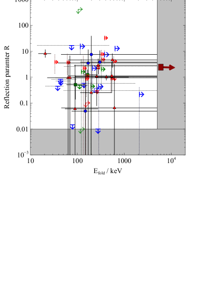
Figure 26.— Reflection parameter $R$ against folding energy $E_{\rm fold}$ from our pexrav fits. Red triangles and small upper/lower limit arrows depict low absorption ($\rm log\thinspace N_{\rm H}\thinspace<22$) objects, blue circles and large upper/lower limit arrows depict high absorption objects ($\rm log\thinspace N_{\rm H}\thinspace>22$) and green squares and intermediate-sized upper/lower-limit arrows represent objects with intermediate absorptions between these two limits. The dark red square shows the mean $R$ and $E_{\rm fold}$ for the whole sample; the ‘formal’ mean $E_{\rm fold}$ lies well outside the BAT band. We plot any objects with $R<0.01$ as an upper limit at $R=0.01$, and for objects $E_{\rm fold}$ above 5000 keV, we treat these fold energies as unobservable and compute a lower limit on $E_{\rm fold}$ using the negative error; these limits are indicated by the gray shaded areas.

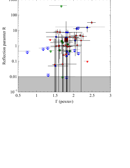
Figure 27.— Reflection parameter $R$ against photon index $\Gamma$ from our pexrav fits. Red triangles and small upper/lower limit arrows depict low absorption ($\rm log\thinspace N_{\rm H}\thinspace<22$) objects, blue circles and large upper/lower limit arrows depict high absorption objects ($\rm log\thinspace N_{\rm H}\thinspace>23$) and green squares and intermediate-sized upper/lower-limit arrows represent objects with intermediate absorptions between these two limits. The dark red square shows the mean $R$ and $\Gamma$ for the whole sample.. We plot any objects with $R<0.01$ as upper limits at $R=0.01$ (emphasized by the gray shaded area).

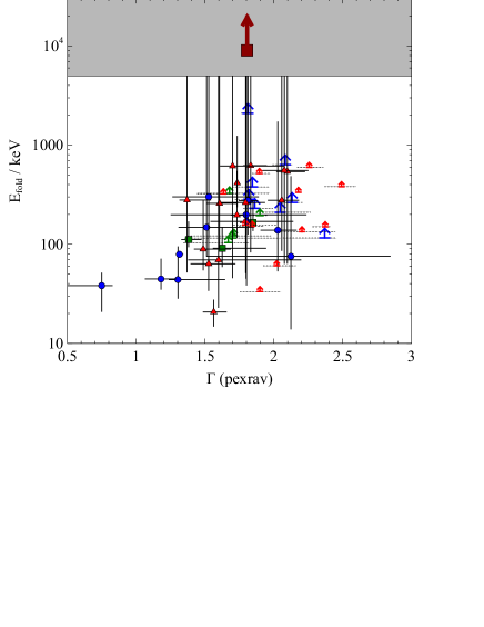
Figure 28.— Folding energy $E_{\rm fold}$ against photon index $\Gamma$ from our pexrav fits. Red triangles and small upper/lower limit arrows depict low absorption ($\rm log\thinspace N_{\rm H}\thinspace<22$) objects, blue circles and large upper/lower limit arrows depict high absorption objects ($\rm log\thinspace N_{\rm H}\thinspace>23$) and green squares and intermediate-sized upper/lower-limit arrows represent objects with intermediate absorptions between these two limits. The dark red square shows the mean $E_{\rm fold}$ and $\Gamma$ for the whole sample. For objects for which the value of $E_{\rm fold}$ is above 5000 keV, we treat them as having an unobservable fold energy outside the BAT band and use the negative error bar to compute a lower limit on $E_{\rm fold}$. The 5000 keV limit is indicated using the gray shaded area.

6. Average Spectrum and log(N)-log(S)

6.1. Stacked Spectrum

We present the stacked/summed spectrum for all sources (excluding the five sources with insufficient counts to construct their spectra) in Fig. 29, for comparison with the corresponding average spectrum generated from the 9-month catalog in W09. While W09 compiled their fits from a variety of different sources in the literature in addition to their own fits, here we have performed a uniform analysis of all of the X-ray spectra for the objects in our sample. We are therefore able to simply sum the model fits to all of the spectra to obtain the stacked spectrum, and avoid the need to employ the complex method outlined in W09. We also distinguish, as done in W09, between the contributions due to simple power-law sources and complex (those with a partial-covering spectral shape) sources. Due to the presence of 13 intermediate-spectral type objects, we produce two versions of the summed spectrum: one assuming all of the intermediate objects are best fit by the simple power-law, and one where all such objects are assumed to have a complex spectrum. The relative importance of the two source types is clearly seen in Fig. 29, but the two versions of the summed spectrum at energies above 0.2 keV show no appreciable differences. Although AGN emission is thought to be responsible for the X-ray background (XRB), the XRB is only well-known for energies $E>0.6$ keV (McCammon et al. 2002, Markevitch et al. 2003, Sołtan 2007, Gupta & Galeazzi 2009). If we fit a power-law to the 1–10 keV region, we find an average power-law slope of $\Gamma=1.37-1.38$, in line with the key finding from W09 that the slope of the XRB below 15 keV found from HEAO-1 ($\Gamma\approx 1.4$) can be reproduced by the summed emission from BAT AGN. We confirm this measurement here with the deeper 58-month catalog, with a greater fraction of obscured AGN (compared to the 9-month catalog), but using a sample that covers 11% of the sky instead of 74% of the sky ( $|b|>15^{\circ}$) from W09. In a companion paper, we extend this stacking analysis to include the BAT data above 10 keV and comment on the relevance of our results to X-ray background studies (Vasudevan et al. 2013 in prep).

Although we do not have data of sufficient quality to detect soft excesses and iron lines in our XRT or ASCA sources ($\sim 50$% of the sample), we find that based solely stacking the objects with XMM-Newton detections, we see both a clear soft excess and an iron line in the summed spectrum for the simple power-law sources (thin solid line in both panels of Fig. 29). The iron line is also notably prominent in the complex spectrum sources (thin dashed line). It would be highly desirable to complete the XMM-Newton-quality coverage for the entire sample to acquire better statistics on the prominence of this feature. This discussion highlights the utility of completing the XMM-Newton coverage of this region of the sky, or obtaining other high-quality data to understand the detailed features in AGN spectra in the Northern Galactic Cap.

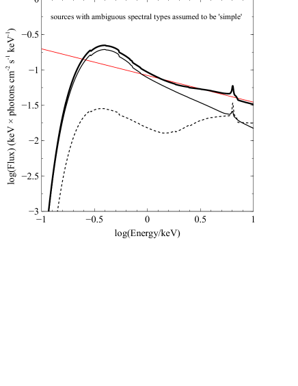
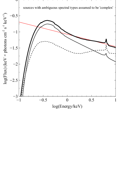
Figure 29.— Summed spectrum for the whole sample. Left panel: the summed spectrum assuming a simple spectral type for any intermediate spectral-type objects. Right panel: the summed spectrum assuming a complex spectral type for such intermediate spectral-type objects. We stack the model spectra for all objects between 0.4–10 keV. The thick black solid line shows the summed overall spectrum in both panels, and the thin solid black and thin dashed black lines show the contributions from simple and complex spectrum-type sources, respectively. The red straight line in both panels shows a fit to the 1–10 keV data (yielding a best-fit photon index of $\Gamma\approx 1.37-1.38$, matching that from the X-ray background).

6.2. log(N)-log(S) diagram

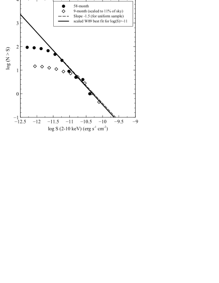
Figure 30.— Plot of log($N>S$) against log($S$), for 2–10 keV flux $S$ in $\rm erg\thinspace s^{-1}\thinspace cm^{-2}$, where log($N>S$) is the logarithm of the number of sources with flux greater than $S$. The thin line shows a slope of $-1.5$ expected for a uniform distribution. Our sample shows a slope consistent with this down to fluxes of log($S$)=$-11.6$.

In order to estimate the completeness of our sample in the 2–10 keV band, we present the 2–10 keV log($N$)-log($S$) plot for the sample in Fig. 30. We adopt all of the same conventions as in W09; $N$ is the number of sources above a threshold 2–10 flux $S$. The slope of the log($N$)-log($S$) relation is expected to be $-1.5$ for a uniform distribution of objects throughout a Euclidean volume (i.e., for low redshifts) with a broad luminosity distribution, and we find our results consistent with this down to a flux of log($S$)$\approx-11.6$ (by inspection; we do not attempt to fit these points due to the complications involved in fitting points with correlated errors). This result contrasts with a completeness limit of log($S$)$\approx-11.0$ from the 9-month catalog, indicating that we have a complete census of objects up to fluxes $\sim 4$ times fainter than the 9-month catalog completeness limit. This log($S$) completeness limit is consistent with the sensitivity expected from the all-sky survey.

Our Northern Galactic Cap sample covers $11$% of the sky, in contrast to $74$% coverage of the sky in the complete sample of W09. In order to more easily compare the results from the 9-month and 58-month catalogs, we therefore scale the results obtained in W09 down to the expected numbers of objects for 11% of the sky, and overplot the scaled 9-month catalog log($N$)-log($S$) relation using empty diamonds in Fig. 30, along with the best fit above log($S$)$\approx-11.0$ from W09. We find that the objects above the W09 completeness limit constitute half of the sample in the 9-month catalog, whereas 65% of our objects lie above our latest completeness limit of log($S$)$\approx-11.6$.

We can also contrast the properties of the source in the ‘complete’ and ‘incomplete’ fractions of the sample from the earlier and later catalogs, in their column density distribution and spectral shapes as done by W09. For clarity, we state that ‘complete’ refers to objects with fluxes log($S$)$>-11.0$ when discussing the 9-month catalog, but refers to objects with log($S$)$>-11.6$ when discussing the 58-month catalog. In order to compare absorption distributions, we redefine any lower-limiting log($N_{\rm H}$)=20 values from W09 to log($N_{\rm H}$)=19 as done in W09. In the 9-month catalog, the objects above completeness show both low absorption ($\langle\rm log\thinspace N_{\rm H}\thinspace\rangle=20.9\pm 0.2$) and a wide range of absorption ($\rm 19.0<log\thinspace N_{\rm H}\thinspace<23.5$), whereas objects above completeness in our latest sample exhibit slightly higher absorption levels ($\langle\rm log\thinspace N_{\rm H}\thinspace\rangle=21.4-21.6\pm 0.2$) and a greater range ($\rm 19.0<log\thinspace N_{\rm H}\thinspace<24.5$), including four Compton-thick candidates. Below completeness, where we expect to be missing a substantial fraction of objects, we find that the incomplete 50% of the 9-month sample has high absorption ($\langle\rm log\thinspace N_{\rm H}\thinspace\rangle=22.5\pm 0.2$) and a wide range ($\rm 19.0<log\thinspace N_{\rm H}\thinspace<24.1$) including two almost-Compton-thick candidates, NGC 1365 and NGC 612, whereas our latest sample shows even higher absorptions below completeness ($\langle\rm log\thinspace N_{\rm H}\thinspace\rangle=22.9-23.2\pm 0.3$) and a wider range ($\rm 19.0<log\thinspace N_{\rm H}\thinspace<25.3$) including the remaining four Compton-thick candidates in our sample. There is larger uncertainty in the average $\rm log(N_{\rm H})$ for objects below completeness since there are more objects with ambiguous spectral types in this regime. Since objects below completeness are by definition fainter, we expect them to have fewer counts in their observations, and therefore require longer exposures before the spectral shape can be properly constrained.

In both the ‘complete’ and ‘incomplete’ regions of our sample, we have a wider range of absorption levels than seen in W09 and a marked increase in the number of Compton-thick candidates (subject to further investigation of their spectra with more physical models). The broad-band spectral shape, as parameterized by the ratio $F_{\rm BAT}/F_{\rm 2-10keV}$, also shows a marked variation. In the 9-month catalog, W09 found indications that the missing sources in the sample were likely to be heavily absorbed since this flux ratio changed from an average $3.0\pm 0.3$ above the completeness flux limit to $16.9\pm 2.3$ in the incomplete part of the sample. This effect is less pronounced in our latest sample: there is a change from $5.3\pm 0.7$ to $12.4\pm 1.9$ for the average value of this flux ratio, indicating that our sample is more homogenous than the previous 9-month catalog.

Below completness, W09 estimate $\sim 3000$ missing objects at log($S$)$\approx-12$, which corresponds to $\sim 400$ sources if scaled to the 11% of sky covered by our Northern Galactic Cap sample. At the same flux level, we are missing $\sim 300$ sources. Based upon the discussion of flux ratios above, it is likely that the missing sources are more heavily absorbed than those above the completeness limit, but since our sample is more homogenous than the 9-month catalog, it is difficult to predict the properties of the missing sources.

7. Results from the Northern Galactic Cap sources in the 22-month BAT catalog

Throughout this paper, all of our results pertain to the 58-month BAT catalog objects in the Northern Galactic Cap. We choose this source list since the 58-month catalog is the deepest edition of the catalog for which the source list and BAT spectra are publicly available. Using the deepest version of the catalog provides the largest possible sample, and therefore allows a more robust determination of the true column density distribution and luminosity distribution. Ideally this requires 0.4–10 keV data of sufficient quality, but high-quality XMM-Newton data is only available for $49\%$ of the objects in our 58-month catalog subsample. However, the 13 new XMM-Newton observations in this sky region from the proposal by PI Brandt were taken to complete XMM-Newton coverage for the 22-month catalog (Tueller et al., 2010) in this sky region, and the observations that were successfully obtained provide XMM-Newton coverage for $90\%$ of the $b>50^{\circ}$ 22-month BAT catalog sources. We therefore present some key comparisons between results for the 9-month catalog (W09’s uniform sample, 102 objects, 74% of the sky), the 22-month catalog (39 objects, 11% of the sky), and the 58-month catalog results (100 objects, 11% of the sky) in Tables 6 and 7 below, to illustrate the utility of the deepening sample, and to identify if any insight can be gained using a complete subsample with higher-quality data. We contrast the flux limits, completeness limits, percentage of sources with ambiguous spectral types, and percentages of objects with different levels/types of absorption in Table 6; we do the same for the luminosity distributions, frequency of spectral features, and percentage of ‘hidden/buried’ sources in Table 7. A few sources in the 22-month catalog list do not occur in the 58-month catalog (due to intrinsic variability of those sources); for our 22-month catalog analysis we only use those sources that survive in the 58-month catalog.

The 22-month catalog flux limit is 1.8 times fainter than the 9-month catalog flux limit, and the 58-month catalog flux limit is 5 times fainter than that for the 9-month. While the 58-month catalog completeness limit (from the $\rm\thinspace logN\thinspace-\thinspace log\thinspace S$ relation) is estimated to be 4 times fainter than the 9-month catalog, the 22-month catalog is only complete to fluxes 1.8 times fainter than the 9-month catalog. Despite the better XMM-Newton coverage for the 22-month catalog subsample, we find that there is still a large degree of uncertainty in the percentages of sources at different absorption levels and with different absorption types (simple/complex) due to four ambiguous spectral-type sources in the 22-month catalog list. The fraction of complex absorption sources appears to change little between the catalogs, within the uncertainties. However, there does seem to be a trend towards uncovering a higher fraction of absorbed sources, in particular Compton-thick objects, as the catalog gets deeper.

The luminosity distributions in all three catalogs show a trend for unabsorbed sources to have marginally brighter luminosities, and percentages of sources with iron K-$\alpha$ lines or soft excess appears relatively stable between the different catalogs. We do not consider warm absorbers here, as this requires a more considered approach; Winter et al. (2012) outline such an approach using XMM-Newton and Suzaku data. In summary, while the 22-month catalog objects in this sky region have better data quality on average, the smaller number of objects in that subset make the percentages presented above more prone to uncertainty.

8. Discussion and Conclusions

We present a detailed X-ray spectral analysis of the non-beamed AGN in the Northern Galactic Cap of the 58-month BAT catalog, consisting of 100 AGN with $b>50^{\circ}$. This field has excellent potential for further investigations due to a wide range of multi-wavelength data that is already available, and we propose the field as a low-redshift analog to the ‘deep field’ observations at higher redshifts (e.g. CDFN/S, Lockman Hole). We present distributions of the redshift, luminosity, absorbing column density and other key quantities for the catalog. We use a consistent approach to fit all data, using our semi-automated X-ray spectral fitting workflow, useful for fitting suites of models to large samples of AGN, producing consistent comparisons between models and determining the significance of various spectral components. In summary, we find that:

• We probe to deeper redshifts with this representative subsample of 100 objects from the 58-month catalog ($\langle z\rangle=0.043$ compared to $0.03$ from W09 and $0.03$ from Burlon et al. 2011)

• The average X-ray luminosity found here ($\langle\rm log\thinspace L_{\rm 2-10keV}\thinspace\rangle=43.0$) is identical to that seen in W09 ($\langle\rm log\thinspace L_{\rm 2-10keV}\thinspace\rangle=43.0$), but with more pronounced tails in the distribution at low and high luminosities. The average 14–195 keV BAT luminosity is $\langle\rm log\thinspace L_{\rm BAT}\thinspace\rangle=43.5$, compared to $43.7$ from W09.

• We uncover a broader absorbing column density distribution. The obscured fraction ($\rm log\thinspace N_{\rm H}\thinspace\geq 22$) is $\sim 60$%, an increase from the measurements for the 36-month catalog (Burlon et al., 2011) and the 9-month catalog (W09). The obscured fraction broadly overlaps with complex spectrum (partial covering-type) sources, which constitute 43-56% of the sample.

• Thirteen objects have ambiguous spectral types in that a unique best-fit model could not be found, and both simple or complex absorption can describe the observed spectral shape. These are typically objects where the existing (generally XRT) data does not have sufficient counts below 1 keV to distinguish between the two models. For these objects, we have presented the results for both models in all subsequent analyses, and take into account the resulting uncertainty in model fit parameters. The most significant uncertainty stemming from these ambiguous sources is the absorbing column density: two different model fits sometimes produce extremely different $\rm log(N_{\rm H})$ values. This behaviour highlights the need to obtain better quality data for these sources.

• We present the properties of iron lines, soft excesses and ionized absorbers detected in the 39 objects with $>4600$ counts in their spectra. Iron lines are detected in 79% of the XMM-Newton objects, similar to 81% found in W09. Soft excesses are detected at a frequency of 31–33% compared to W09’s 41%, and ionized absorption edges are detected in 18% of our sample. We present upper limiting iron line equivalent widths for sources where the feature was not detected as a significant addition to the spectrum, and confirm the X-ray Baldwin effect to the degree identified by e.g., Page et al. (2004) in our sample.

• We introduce the concept of the soft-excess strength, defined as the luminosity in the soft excess (modelled as a black body) divided by the power-law luminosity between the ‘clean range’ 1.5–6 keV. In W09, a linear relation was found between the soft excess power and power-law luminosity. We find a deviation from this description, suggesting that the soft excess is not simply powered by the power-law coronal emission, as the fraction of power seen in the soft excess drops slightly at higher power-law luminosities. We also find a disjoint distribution of sources: one set in which a soft excess is well-detected and for which the soft excess fraction is $>0.1$, and another family of sources where the soft excess is not detected at all (indicated by stringent upper limits in the soft-excess strength). This result suggests that the process responsible for producing the soft excess is not ubiquitous in AGN.

• The fraction of unabsorbed ($\rm log\thinspace N_{\rm H}\thinspace<22$) sources with ionized absorber edges is $\sim 32\%$, lower than the $53\%$ found for Seyfert 1–1.5 BAT AGN in Winter et al. (2012). However, given that our study and previous studies estimating the prevalence of ionized absorbers have small sample sizes, our result is broadly consistent with previous results.

• The fraction of Compton-thick sources ($\rm log\thinspace N_{\rm H}\thinspace>24.15$) in our sample is $\sim 9$%, using a simple absorption model (ztbabs). Other measures of Compton thickness, such as high Fe-K line equivalent width, high reflection $R$ or a flat photon index (pegging at $1.5$), were also investigated, which may add 2–6 Compton thick candidates, increasing the proportion of such sources to 11–15%. The true Compton-thick fraction involves estimating the number missed due to the attenuation of Compton-thick AGN spectra in the BAT band. Burlon et al. (2011) suggest that the true Compton-thick fraction could be 20%.

• We identify seven new ‘hidden’ sources, unidentified in W09, three by using newly obtained XMM-Newton data. The fraction of such sources in our sample is 13–14%, lower than the proportion found in W09.

• Reflection is found to be important in a large fraction of our sample, with the average value of the reflection fraction found to be $\langle R\rangle=2.7\pm 0.75$, suggestive of strong light bending or highly complex absorption. The average fold energy of the sample is well outside the BAT band, but we do observe a well-defined high-energy cut-off in some sources. The use of BAT data in conjunction with XMM-Newton data allows reflection parameters to be better constrained, and our technique for re-normalizing the BAT data (using the BAT light curves) to the epoch during which the 0.4–10 keV data were taken removes a degree of freedom from the fit, further constraining the fit for some objects.

• We present the summed spectrum for the sample. The slope of the summed spectrum between 1–10 keV reproduces the X-ray background slope, as found in W09, but we find this with a deeper sample that exhibits a different absorption distribution. Iron lines and soft excesses appear to be significant in the whole sample, but higher quality data are needed for about half the sample (that does not yet have XMM-Newton coverage) to understand the frequency of these components properly.

• The 2–10 keV log($N$)-log($S$) plot for the Northern Galactic Cap reveals completeness down to log($S$)$\approx-11.6$, a factor of $\sim 4$ fainter than the 9-month catalog. A larger proportion of our sources lie above the completeness limit than in W09, and whilst the missing sources are expected to be more heavily absorbed and possibly Compton-thick due to their $F_{\rm BAT}/F_{\rm 2-10keV}$ ratio, the absorption properties of our 58-month BAT catalog subsample seem to be more homogenous both above and below completeness than found in W09 for the 9-month catalog.

• We consider the properties of the complete subsample of 39 objects drawn from the 22-month BAT catalog source list in this sky region, for which the XMM-Newton coverage is 90% (compared to 49% for our full 58-month sample), to identify whether the improved data quality allows more robust determination of the subsample properties. However, we do not find significantly more stringent constraints on fractions of complex spectra, luminosity distributions, or the proportions of sources with iron lines and soft excesses. This is in part due to the smaller sample size of the 22-month subset and four sources in the 22-month catalog with ambiguous spectral types. There is some evidence, however, for an increasing fraction absorbed (including Compton-thick sources) with survey depth.

In summary, we have analysed an unbiased sample that is representative of local AGN activity spanning a wide range of parameters (absorption, luminosity), with detailed information on the X-ray properties of the sample. There is substantial scope to build a suite of multi-wavelength studies on this sample, to further our understanding of AGN accretion at $z<0.2$. We defer some of the following issues to later studies, for brevity. The complete sample assembled here will provide a useful base for understanding long-term AGN variability, by analysing multi-epoch observations of these AGN; many such observations exist in the archives, and such a study would complement other such variability studies on AGN samples (e.g., Paolillo et al. 2004). It would also be interesting to examine low-energy X-ray emission (below $\sim$1 keV) in buried AGNs for potential signatures of hot-gas emission due to nuclear starburst or broader galactic activity. We again remind the reader of the existing multi-band coverage and therefore potential for generating broad-band SEDs and accretion rates, which we identify as a key priority for future work. We are currently working on companion studies related to understanding reflection in AGN; including a study of correlations between soft X-ray features (soft excesses, iron lines) and the Compton reflection hump. Our previous studies using the BAT catalog (Mushotzky et al. 2008, W09, Vasudevan et al. 2009, 2010) all reveal the complexities of determining accurate black-hole mass estimates for this sample; an object-specific approach is required to determine black-hole masses in a diverse AGN sample such as this, making this another priority for the future.

9. Acknowledgements

RVV would like to thank Jeremy Sanders for designing and providing extensive support for the Veusz plotting package with which most of the plots in this paper were generated, and Mike Koss for his comments on the paper. We thank Jack Tueller, Craig Markwardt and Neil Gehrels for their work on the proposal to extend the XMM-Newton coverage of this region, and all of the BAT team for their work on the BAT catalog. We also thank the anonymous referee for useful comments that improved the paper. This work makes use of data from XMM-Newton, an ESA science mission with instruments and contributions directly funded by ESA Member States and NASA. This research has made use of the NASA/IPAC Extragalactic Database (NED) which is operated by the Jet Propulsion Laboratory, California Institute of Technology, under contract with the National Aeronautics and Space Administration (NASA).

Appendix A APPENDIX: Moderately radio loud sources Mrk 463 and 3C 303.0

The objects Mrk 463 and 3C 303.0 were identified as having the highest radio loudness parameters in the sample ($RL\gtrsim-3$). It is not straightforward to account for how this will affect the X-ray spectral fitting, since the radio emission could be due to a combination of star formation (e.g., Condon et al. 2002) and jet emission. In the case of Mrk 463, this is a known dual AGN system (§4.2) the radio images available on NED for this object reveal a non-standard morphology for the radio source which cannot be straightforwardly classified as one of the traditional Fanaroff-Riley classes (FR-I/FR-II). There is little evidence for a significant component of X-ray jet emission in radio-loud non-blazar AGN (Sambruna et al., 1999), and indeed the X-ray analysis of Mrk 463 in Bianchi et al. (2008) does not consider any X-ray component in the Chandra or XMM-Newton data. For 3C 303.0, we inspect the archival Chandra images and find that while the 2–10 keV emission has a negligible contribution from extended jet emission, the 0.5–2 keV emission may be contaminated by jet emission at a level of $17\%$ of the nuclear emission. This is likely to influence our spectral fit for this object. However, inspection of the spectrum reveals a smooth power law from 0.5–10 keV. If the intrinsic nuclear spectrum is more heavily absorbed, the radio emission due to jets at soft energies may give the illusion of less absorption. However, determining the precise degree of jet contamination is complex, and since these considerations only affect two of our objects, they will not influence the absorption distributions and other results significantly.

Appendix B APPENDIX: Sources with low counts

The five sources in Table 8 had XRT data but lacked sufficient counts to construct a spectrum, and due to their poor data quality we have not included them when calculating sample-wide properties presented in this paper. For completeness, we present a basic analysis of these datasets here. We examined the counts in the 0.5–2 keV and 2–10 keV in the source and background regions for these objects. When sources were detected at a $\geq 2\sigma$ level above background, we calculate basic fluxes and luminosities (in 0.5–2 and 2–10 keV bands) using WebPIMMS assuming a Galactic-absorbed powerlaw with a photon index of $1.9$; where the sources were not detected at greater than $2\sigma$, we present 95% confidence upper limits on fluxes and luminosities. These upper limits were calculated using the Gehrels (1986) prescription. These sources would clearly benefit from longer, higher signal-to-noise ratio observations to identify whether there is any sustained X-ray emission.

We attempt to recover an estimate for the intrinsic column density in these sources, since the very faint X-ray fluxes may be indicative of heavily absorbed, potentially Compton-thick objects, when considered alongside the available BAT spectra. However, we find that this approach produces uncertain results with large uncertainties on the inferred log($N_{\rm H}$), unless we are able to renormalize the BAT spectrum and thereby have a better estimate of the absolute ratio between the 2–10 keV and 14–195 keV fluxes (only possible for three of these objects). These results are presented in the final column of Table 8 for completeness. We do not find any convincing hints of Compton-thick candidates amongst these five objects, but better data are needed.

Appendix C APPENDIX: Poor fits

From the 95 with spectra with sufficient counts to attempt fitting, we identify 19 which have null-hypothesis probabilities of their best-fitting models less than $5\times 10^{4}$, indicating that some key features of these spectra have not been modeled fully. In this work, we do not attempt to account for all of the detail in each spectrum, but try to account for the key properties of the spectrum such as the photon index, intrinsic absorption, and the basic set of features discussed in §4.7 and restrict ourselves to these features. AGN spectra often exhibit much more complexity than the model combinations used here, and we examine if this complexity can account for the poor fits in the 19 sources with low null-hypothesis probabilities. On inspection, these objects can be split into three categories: 1) those with few counts, 2) partial covering sources with un-modelled residuals at low energies, such as bumps or other types of structure below 1 keV, and 3) sources with broad iron lines with complex structure not modelled by the zgauss model, which were already discussed above. The soft features in the second category may be due to features in the host galaxies of these AGN (such as emission lines from photo-ionized/hot gas), but are not addressed further here.

AGN	Redshift	RA	Dec	$l$	$b$	Instrument	Obs. ID	Obs.	Source	Obs.	Usable	Optical
								date	Counts	time (ks)	$\%$ of obs.	Type	BAT flux (SNR)
3C 234	0.1849	150.457	28.785	200.208	52.708	XMM	0405340101	2006-04-24	9214	$39.9$	$84$	Sy1/Sy2	8.73 (5.10)
NGC 3227	0.0039	155.878	19.865	216.992	55.446	XMM	0101040301	2000-11-28	53612	$40.1$	$99$	Sy1.5	112.78 (56.21)
SDSS J104326.47+110524.2	0.0476	160.860	11.089	234.761	55.932	XRT	00040954001	2010-10-29	2085	$9.8$	–	Sy1	14.85 (4.84)
MCG +06-24-008	0.0259	161.203	38.181	182.222	61.326	XRT	00040955004	2010-10-31	133	$4.4$	–	galaxy	13.69 (5.04)
UGC 05881	0.0206	161.679	25.932	208.222	62.148	XRT	00037314002	2008-07-03	217	$8.8$	–	Sy2	20.94 (10.42)
Mrk 417	0.0328	162.379	22.964	214.722	62.143	XMM	0312191501	2006-06-15	1788	$14.3$	$75$	Sy2	33.63 (15.22)
2MASX J10523297+1036205	0.0878	163.137	10.606	237.757	57.525	XRT	00037131004	2008-07-13	190	$16.2$	–	Sy1	17.52 (6.63)
Mrk 728	0.0356	165.258	11.047	239.366	59.481	XMM	0103861801	2002-05-23	21479	$9.7$	$100$	Sy1.9	11.90 (5.17)
FBQS J110340.2+372925	0.0739	165.918	37.490	181.567	65.101	XRT	00039831001	2009-07-12	1049	$8.2$	–	Sy1	8.86 (5.38)
2MASX J11053754+5851206	0.1930	166.407	58.856	145.639	53.357	XRT	00040957001	2010-08-30	910	$11.2$	–	QSO/BLAGN	5.52 (4.97)
CGCG 291-028	0.0477	166.496	58.946	145.481	53.320	XRT	00040957001	2010-08-30	46	$11.2$	–	Sy2	4.37 (4.97)
IC 2637	0.0292	168.457	9.586	245.603	61.057	XMM	0601780201	2009-12-20	31401	$15.1$	$100$	Sy1.5	15.16 (6.40)
MCG +09-19-015	0.0703	168.833	54.389	149.169	57.569	XRT	00031290001	2008-11-07	94	$4.6$	–	Sy2	9.08 (5.58)
PG 1114+445	0.1438	169.277	44.226	164.675	64.494	XMM	0109080801	2002-05-14	42913	$43.5$	$97$	Sy1	8.93 (4.93)
ARP 151	0.0211	171.401	54.383	147.029	58.546	XRT	00037369002	2009-02-15	3076	$8.1$	–	Sy1	17.81 (11.05)
1RXS J1127+1909	0.1055	171.818	19.156	230.898	69.111	XMM	0601780301	2009-05-29	25011	$11.9$	$100$	Sy1.8	16.84 (8.59)
UGC 06527	0.0274	173.170	52.949	147.136	60.320	XMM	0200430501	2004-05-02	976	$12.7$	$95$	Sy2	8.09 (7.32)
IC 2921	0.0437	173.205	10.296	251.453	64.978	XRT	00038055002	2010-07-23	781	$8.6$	–	Sy1	17.51 (7.12)
NGC 3758	0.0299	174.123	21.596	226.837	72.080	XMM	0601780401	2009-06-14	30020	$11.9$*	$100$	Sy1	11.46 (8.16)
SBS 1136+594	0.0601	174.786	59.198	139.255	55.580	XRT	00035265001	2005-12-14	3521	$9.2$	–	Sy1.5	20.85 (12.12)
Mrk 744	0.0089	174.928	31.909	191.584	73.704	XMM	0204650301	2004-05-24	10239	$29.5$	$42$	Sy1.8	20.49 (8.70)
PG 1138+222	0.0632	175.317	21.939	227.137	73.238	XRT	00037371001	2008-10-26	2693	$9.1$	–	Sy1	17.19 (8.13)
2E 1139.7+1040	0.1505	175.570	10.394	255.411	66.650	XRT	00036986001	2008-07-23	25	$1.6$	–	Sy1	15.75 (7.21)
KUG 1141+371	0.0381	176.125	36.886	174.169	72.821	XMM	0601780501	2009-05-23	17251	$19.8$	$66$	Sy1	15.47 (5.93)
MCG+10-17-061	0.0099	176.387	58.977	138.147	56.162	XRT	00038346001	2009-02-17	435	$8.9$	–	galaxy	15.99 (9.36)
2MASX J11475508+0902284	0.0688	176.980	9.041	260.274	66.498	XRT	00040962001	2010-07-02	1357	$8.9$	–	Sy1.5	11.06 (6.38)
MCG +05-28-032	0.0230	177.190	29.642	198.919	75.999	XRT	00090176001	2009-10-20	139	$2.7$	–	LINER	23.79 (10.20)
2MASX J11491868-0416512	0.0845	177.327	-4.280	275.039	55.192	XRT	00038057001	2009-11-09	634	$5.0$	–	Sy1	11.83 (5.99)
MCG -01-30-041	0.0188	178.160	-5.208	277.014	54.678	XRT	00037373002	2009-08-04	44	$6.0$	–	Sy1.8	13.69 (5.64)
NGC 3998	0.0035	179.484	55.453	138.172	60.064	XMM	0090020101	2001-05-09	37289	$13.2$*	$94$	Sy1/LINER	16.89 (9.83)
CGCG 041-020	0.0360	180.242	6.806	270.116	66.407	XMM	0312191701	2006-06-26	7098	$12.9$	$100$	Sy2	21.18 (9.61)
MRK 1310	0.0194	180.310	-3.678	279.540	56.896	XRT	00035361001	2005-12-25	1789	$6.3$	–	Sy1	13.23 (6.11)
NGC 4051	0.0023	180.791	44.531	148.882	70.085	XMM	0157560101	2002-11-22	147191	$51.9$*	$86$	Sy1.5	37.62 (24.17)
Ark 347	0.0224	181.124	20.316	242.830	77.289	XRT	00035599002	2006-07-04	141	$10.4$	–	Sy2	29.15 (11.73)
PG 1202+281	0.1653	181.176	27.902	205.968	79.613	XMM	0109080101	2002-05-30	57522	$17.9$	$100$	Sy1.2	9.99 (5.79)
UGC 7064	0.0250	181.180	31.177	188.499	79.034	XMM	0601780601	2009-12-26	15499	$39.5$	$88$	Sy1.9	13.64 (5.28)
2MASX J12055599+4959561	0.0631	181.483	49.999	140.753	65.525	XRT	00040963001	2010-04-26	204	$7.8$	–	BLAGN	12.37 (5.30)
NGC 4102	0.0028	181.596	52.711	138.079	63.072	XMM	0601780701	2009-10-30	2085	$31.8$	$41$	LINER	28.55 (14.07)
B2 1204+34	0.0791	181.887	33.879	174.707	78.396	XRT	00037315003	2008-10-20	110	$8.6$	–	Sy2	16.91 (5.04)
Mrk 198	0.0242	182.309	47.059	142.750	68.413	XMM	0601780801	2009-11-07	15537	$26.9$	$92$	Sy2	21.94 (12.32)
NGC 4138	0.0030	182.374	43.685	147.305	71.404	XMM	0112551201	2001-11-26	7674	$15.0$	$100$	Sy1.9	30.67 (14.92)
NGC 4151	0.0033	182.637	39.406	155.074	75.064	XMM	0112310101	2000-12-21	247586	$33.0$	$100$	Sy1.5	533.09 (275.00)
KUG 1208+386	0.0228	182.686	38.336	157.646	75.920	XMM	0601780901	2009-06-14	3691	$15.8$	$71$	Sy1	21.63 (12.63)
NGC 4180	0.0070	183.262	7.038	276.792	67.940	XRT	00036654002	2007-11-30	7	$3.0$	–	AGN	14.44 (6.04)
2MASX J12135456-0530193	0.0660	183.477	-5.506	286.006	56.128	XRT	00040964003	2010-11-21	534	$4.0$	–	Sy1	11.94 (5.18)
Was 49b	0.0640	183.574	29.529	194.394	81.484	ASCA	73036000	1995-05-22	1693	$39.6$	–	Sy2/binary AGN	15.40 (7.96)
NGC 4235	0.0080	184.292	7.191	279.183	68.468	XMM	0204650201	2004-06-09	13865	$13.1$	$100$	Sy1	31.39 (14.07)
Mrk 202	0.0210	184.479	58.660	131.140	57.931	ASCA	77076000	09-11-1999	4519	$20.0$	–	Sy1	8.07 (4.82)
Mrk 766	0.0129	184.611	29.813	190.681	82.271	XMM	0304030101	2005-05-23	454079	$95.5$	$91$	Sy1.5	21.42 (14.64)
NGC 4258	0.0015	184.740	47.304	138.319	68.842	XMM	0059140101	2001-05-06	10415	$12.7$	$100$	Sy1.9/LINER	23.92 (11.71)

Table 1Observations

AGN	Redshift	RA	Dec	$l$	$b$	Instrument	Obs. ID	Obs.	Source	Obs.	Usable	Optical
								date	Counts	time (ks)	$\%$ of obs.	Type	BAT flux (SNR)
Mrk 50	0.0234	185.851	2.679	286.395	64.647	XMM	0601781001	2009-07-09	64116	$11.9$*	$100$	Sy1	23.95 (10.18)
NGC 4388	0.0084	186.445	12.662	279.123	74.335	XMM	0110930301	2002-07-07	3629	$18.8$	$78$	Sy2	275.78 (110.73)
NGC 4395	0.0011	186.455	33.546	162.095	81.534	XMM	0112521901	2002-05-31	11194	$15.9$	$97$	Sy1.9	26.08 (14.28)
NGC 4500	0.0104	187.842	57.965	128.094	58.962	XRT	00040965001	2010-04-25	24	$4.5$	–	starburst galaxy?	8.69 (5.78)
Ark 374	0.0630	188.016	20.158	269.447	81.739	XMM	0301450201	2005-07-09	95204	$25.5$	$100$	Sy2	14.84 (6.17)
NGC 4579	0.0051	189.432	11.818	290.398	74.355	XMM	0112840101	2003-06-12	79300	$23.7$	$100$	LINER	10.41 (4.93)
NGC 4593	0.0090	189.914	-5.344	297.483	57.403	XMM	0109970101	2000-07-02	278937	$28.1$	$80$	Sy1	88.68 (33.45)
NGC 4619	0.0231	190.436	35.063	136.975	81.799	ASCA	75081000	1997-06-03	3179	$33.4$	–	Sy1	6.64 (5.59)
NGC 4686	0.0167	191.669	54.534	124.432	62.581	XMM	0554500101	2008-06-28	1350	$30.3$	$62$	XBONG	27.88 (13.12)
2MASX J13000533+1632151	0.0800	195.024	16.537	314.092	79.220	XMM	0149170701	2003-07-14	1136	$6.4$	$69$	Sy1?	14.83 (5.31)
MCG -01-33-063	0.0263	195.080	-8.086	306.739	54.720	XRT	00041773002	2010-12-08	10	$2.6$	–	galaxy	10.32 (4.92)
MRK 0783	0.0672	195.746	16.407	317.528	78.950	XRT	00037318001	2008-05-09	679	$5.8$	–	Sy1.5	17.93 (9.00)
SWIFT J1303.9+5345	0.0299	196.000	53.791	118.811	63.237	XMM	0312192001	2006-06-23	64141	$11.9$*	$100$	Sy1	34.56 (18.53)
NGC 4941	0.0037	196.055	-5.552	308.806	57.174	ASCA	74040000	1996-07-19	567	$17.1$	–	Sy2	19.41 (7.41)
NGC 4939	0.0104	196.059	-10.338	308.096	52.405	XRT	00031153005	2008-03-07	65	$6.6$	–	Sy2	25.43 (8.38)
SWIFT J1309.2+1139	0.0251	197.274	11.633	318.766	73.960	XMM	0312192101	2006-06-27	2365	$16.4$	$98$	XBONG	55.64 (21.63)
2MASX J13105723+0837387	0.0527	197.738	8.627	317.846	70.932	XRT	00041174001	2010-08-20	50	$8.8$	–	Sy2	10.94 (5.19)
II SZ 010	0.0343	198.274	-11.128	311.463	51.384	XRT	00037378001	2009-02-25	1855	$4.8$	–	Sy1	14.55 (5.71)
NGC 5033	0.0029	198.365	36.594	98.060	79.448	XMM	0094360501	2002-12-18	34064	$11.9$	$100$	Sy1.9	6.95 (5.27)
UGC 08327 NED02	0.0366	198.823	44.407	108.983	72.069	XRT	00037093003	2007-09-20	152	$2.4$	–	Sy2	16.79 (10.92)
NGC 5106	0.0319	200.246	8.980	325.355	70.554	XRT	00038063001	2009-11-23	73	$6.9$	–	AGN	13.97 (5.51)
NGC 5231	0.0218	203.951	2.999	328.569	63.640	XMM	0601781201	2010-01-30	13934	$17.9$	$100$	Sy2	17.24 (7.46)
NGC 5252	0.0230	204.567	4.543	331.299	64.803	XMM	0152940101	2003-07-18	84375	$67.3$	$78$	Sy1.9	111.13 (42.40)
Mrk 268	0.0399	205.297	30.378	52.466	78.630	XMM	0554500701	2008-07-20	6135	$28.5$	$76$	Sy2/gal. pair	18.97 (10.14)
NGC 5273	0.0035	205.535	35.654	74.348	76.246	XMM	0112551701	2002-06-14	25885	$17.1$	$100$	Sy1.9	14.15 (5.41)
CGCG 102-048	0.0269	206.065	19.567	3.747	75.726	XRT	00037319001	2008-06-25	3	$0.3$	–	Sy1.9	20.01 (7.62)
NGC 5290	0.0086	206.330	41.713	89.276	71.714	XRT	00038067001	2008-09-05	589	$5.6$	–	Sy2	19.14 (8.05)
2MASX J13462846+1922432	0.0840	206.618	19.379	4.296	75.190	XRT	00090327001	2010-04-04	629	$5.3$	–	galaxy	10.71 (6.54)
UM 614	0.0327	207.470	2.079	334.600	61.305	XMM	0601781301	2010-01-31	3132	$19.8$	$34$	Sy1	16.18 (6.77)
2MASX J13542913+1328068	0.0635	208.621	13.467	353.206	69.912	XRT	00040970001	2010-06-01	39	$3.4$	–	galaxy	9.70 (5.00)
2MASX J13553383+3520573	0.1016	208.892	35.350	67.887	74.047	XRT	00040971001	2010-08-26	135	$7.2$	–	galaxy	7.31 (4.91)
Mrk 464	0.0501	208.973	38.575	77.329	72.322	XMM	0072340701	2002-12-10	11416	$8.1$	$100$	Sy1.5	20.26 (10.35)
Mrk 463	0.0504	209.011	18.371	5.821	72.747	XMM	0094401201	2001-12-22	4022	$26.8$	$90$	Sy1/dual AGN	11.61 (5.22)
NGC 5506	0.0062	213.313	-3.208	339.150	53.809	XMM	0201830201	2004-07-11	122599	$21.6$	$100$	Sy1.9	242.76 (95.00)
NGC 5548	0.0172	214.499	25.137	31.960	70.495	XMM	0089960301	2001-07-09	1875711	$95.8$	$97$	Sy1.5	73.57 (32.55)
H 1419+480	0.0723	215.376	47.790	88.564	62.886	XMM	0094740201	2002-05-27	59341	$21.5$	$55$	Sy1.5	19.42 (10.55)
NGC 5610	0.0169	216.095	24.615	31.299	68.973	XRT	00090180002	2009-11-18	232	$5.8$	–	Sy2	19.30 (9.15)
Mrk 813	0.1105	216.854	19.831	19.700	66.861	XRT	00035307003	2007-01-10	1873	$6.2$	–	Sy1	12.29 (6.23)
Mrk 1383	0.0865	217.278	1.285	349.218	55.125	XMM	0102040501	2000-07-28	22461	$17.6$	$100$	Sy1	17.66 (7.16)
NGC 5674	0.0249	218.469	5.459	355.897	57.383	XRT	00040977001	2010-09-10	320	$6.0$	–	Sy1.9	13.61 (5.71)
NGC 5683	0.0362	218.719	48.662	86.979	60.615	XRT	00038070002	2010-11-12	175	$10.4$	–	Sy1	13.39 (7.99)
Mrk 817	0.0315	219.093	58.794	100.299	53.478	XMM	0601781401	2009-12-13	61638	$14.2$*	$75$	Sy1.5	27.39 (15.65)
2MASX J14391186+1415215	0.0714	219.799	14.256	11.223	61.795	XRT	00037321001	2008-04-27	163	$4.7$	–	XBONG	15.79 (6.53)
Mrk 477	0.0377	220.159	53.504	93.037	56.819	ASCA	73028000	1995-12-04	871	$21.4$	–	Sy1	13.44 (7.71)
3C 303.0	0.1412	220.761	52.027	90.528	57.501	ASCA	73008000	1995-05-22	3131	$18.2$	–	Sy1.5/FR-II	8.12 (4.90)
2MASX J14530794+2554327	0.0490	223.283	25.910	37.352	62.817	XRT	00037322001	2008-02-01	1613	$4.2$	–	Sy1	23.43 (10.56)
Mrk 841	0.0364	226.006	10.437	11.209	54.631	XMM	0112910201	2001-01-13	128688	$10.1$	$100$	Sy1	36.08 (14.55)
MRK 1392	0.0361	226.485	3.708	2.754	50.264	XRT	00037323001	2008-12-23	764	$5.8$	–	Sy1	18.81 (7.70)
2MASX J15064412+0351444	0.0377	226.682	3.863	3.137	50.211	XRT	00036622001	2007-12-19	472	$9.4$	–	Sy2	16.77 (7.70)
NGC 5899	0.0085	228.763	42.050	69.398	57.216	XMM	0651850501	2011-02-13	14459	$22.9$	$100$	Sy2	20.95 (9.67)

Table 1: Table of observations used for each object (continued).

Model identifier	xspec model string	Description
Simple power-law models
S1	tbabs(powerlaw)	Power-law with Galactic absorption only
S2	tbabs(ztbabs(powerlaw))	Absorbed power-law with Galactic and intrinsic (neutral) absorption
S3	tbabs(ztbabs(powerlaw+zgauss))	As for S2, with a Fe K-$\alpha$ line at (default) 6.4 keV
S4	tbabs(ztbabs(powerlaw+zbbody))	As for S2, with a soft excess modelled as a black body
S5	tbabs(ztbabs(zedge(powerlaw)))	As for S2, with an edge at 0.73 keV (default) to model a warm absorber
S6	tbabs(ztbabs((powerlaw+zbbody+zgauss)))	As for S2, with both a soft excess and Fe K-$\alpha$ line
S7	tbabs(ztbabs(zedge(powerlaw+zgauss)))	Absorbed power-law with warm absorber edge and Fe K-$\alpha$ line
S8	tbabs(ztbabs(zedge(powerlaw+zgauss+zbbody)))	Absorbed power-law with warm absorber edge, Fe K-$\alpha$ line and soft excess
S9	tbabs(ztbabs(zedge(zedge(powerlaw))))	Absorbed power-law with two warm absorber edges at 0.73 and 0.87 keV (default energies)
S10	tbabs(ztbabs(zedge(zedge(powerlaw+zgauss))))	Absorbed power-law with two warm absorber edges and a Fe K-$\alpha$ line
S11	tbabs(ztbabs(zedge(zedge(powerlaw+zgauss+zbbody))))	Absorbed power-law with two warm absorber edges, Fe K-$\alpha$ line and soft excess
Complex models (partial covering)
C1	tbabs(zpcfabs(powerlaw))	Partially-covered absorbed power-law with Galactic absorption
C2	tbabs(zpcfabs(powerlaw+zgauss))	As for C1, including a Fe K-$\alpha$ line at (default) 6.4 keV

Table 2 Model combinations used

AGN	Model ($\chi^{2}/\rm d.o.f$, $P(null\thinspace hyp.)$)	$N_{\rm H}^{\rm Gal}$	$N_{\rm H}$ (covering fraction)	$\Gamma$	$F_{\rm 0.5-2keV}$	$F_{\rm 2-10keV}$	$L^{\rm int}_{\rm 0.5-2keV}$	$L^{\rm int}_{\rm 2-10keV}$	$L_{\rm 14-195keV}$	$RL=L_{\rm 5GHz}/L_{\rm 2-10keV}^{\rm int}$
	(1)	(2)	(3)	(4)	(5)	(6)	(7)	(8)	(9)	(10)
3C 234	C2 (658.26/361, 0.000)	$1.76$	$23.81^{+0.02}_{-0.02}\thinspace(0.98)$	$2.20_{-0.01}$	0.94	12.54	44.70	$44.64^{+0.02}_{-0.00}$	44.9 (44.6$\dagger$)	$<-5.331$
NGC 3227	C2 (1988.13/1775, 0.000)	$1.99$	$23.02^{+0.01}_{-0.01}\thinspace(0.92)$	$1.50^{+0.01}$	3.83	84.25	41.18	$41.58^{+0.01}_{-0.02}$	42.6 (42.7)	$-3.917$
SDSS J104326.47+110524.2	S2+BAT (80.53/89, 0.728)	$2.47$	$20.82^{+0.19}_{-0.32}$	$1.83^{+0.10}_{-0.09}$	29.18	51.99	43.26	$43.43^{+0.10}_{-0.10}$	43.9 (43.8)	$<-5.403$
MCG +06-24-008	C1+BAT (4.72/7, 0.694)	$1.26$	$23.81^{+0.55}_{-1.26}\thinspace(0.79^{+0.21}_{-0.48})$	$1.50^{+0.46}$	9.04	46.06	42.81	$43.20^{+0.90}_{-0.81}$	43.3 (43.3)	$-4.895$
MCG +06-24-008	S2+BAT (6.04/8, 0.643)	$1.26$	$22.96^{+0.31}_{-1.05}$	$1.50^{+0.38}$	0.18	34.11	42.46	$42.85^{+0.33}_{-0.47}$	43.3 (43.3)	$-4.671$
UGC 05881	C1+BAT (7.81/13, 0.856)	$2.51$	$24.39^{+0.15}_{-0.14}\thinspace(0.92^{+0.03}_{-0.09})$	$2.05^{+0.15}_{-0.31}$	22.63	33.48	43.44	$43.47^{+0.48}_{-43.47}$	43.3 (43.6$\dagger$)	$-5.245$
Mrk 417	C1+BAT (129.03/81, 0.001)	$1.88$	$24.08^{+0.02}_{-0.02}\thinspace(0.99)$	$1.87^{+0.04}_{-0.04}$	0.51	16.35	43.36	$43.51^{+0.07}_{-0.07}$	43.9 (43.9$\dagger$)	$<-5.798$
2MASX J10523297+1036205	C1+BAT (10.65/12, 0.559)	$2.29$	$24.41^{+0.23}_{-0.18}\thinspace(0.89^{+0.07}_{-0.09})$	$1.63^{+0.40}_{-1.63}$	6.89	19.25	44.08	$44.38^{+0.62}_{-0.56}$	44.5 (45.0$\dagger$)	$-5.277$
Mrk 728	S3 (616.39/633, 0.674)	$2.02$	–	$1.77^{+0.03}_{-0.02}$	21.34	37.28	42.80	$43.03^{+0.02}_{-0.03}$	43.5 (43.5)	$-4.872$
FBQS J110340.2+372925	S2+BAT (52.36/49, 0.345)	$1.64$	$<20.95$	$1.69^{+0.15}_{-0.12}$	16.84	33.94	43.37	$43.64^{+0.14}_{-0.15}$	44.1 (44.2$\dagger$)	$-4.442$
2MASX J11053754+5851206	C1+BAT (17.93/39, 0.998)	$0.61$	$22.26^{+0.19}_{-0.29}\thinspace(0.61^{+0.07}_{-0.15})$	$2.19^{+0.01}_{-0.31}$	10.35	16.65	44.33	$44.27^{+0.22}_{-0.18}$	44.8 (44.5)	$<-4.961$
2MASX J11053754+5851206	S2+BAT (25.06/40, 0.969)	$0.61$	$<20.86$	$1.71^{+0.15}_{-0.08}$	10.22	18.76	44.01	$44.27^{+0.11}_{-0.12}$	44.8 (44.5)	$<-4.930$
CGCG 291-028	S2+BAT (8.81/7, 0.266)	$0.61$	$23.87^{+0.17}_{-0.30}$	$2.20*$	0.00	6.63	43.34	$43.28^{+0.47}_{-0.68}$	43.4 (43.5)	$<-4.342$
IC 2637	S6 (804.05/786, 0.320)	$2.23$	–	$1.69^{+0.04}_{-0.04}$	16.97	29.92	42.53	$42.75^{+0.04}_{-0.05}$	43.5 (43.2$\dagger$)	$-3.998$
MCG +09-19-015	C1+BAT (3.28/6, 0.773)	$0.78$	$<25.23\thinspace(0.64*)$	$1.95^{+0.25}_{-0.43}$	9.90	19.37	43.51	$43.61^{+0.74}_{-43.61}$	44.0 (43.9$\dagger$)	$<-5.191$
MCG +09-19-015	S2+BAT (3.63/7, 0.821)	$0.78$	$<23.39$	$1.80^{+0.36}_{-0.29}$	0.25	17.69	43.26	$43.46^{+0.70}_{-43.46}$	44.0 (43.9$\dagger$)	$<-5.091$
PG 1114+445	S10 (1254.56/1133, 0.007)	$1.77$	–	$1.50^{+0.01}$	5.52	22.33	43.66	$44.06^{+0.01}_{-0.01}$	44.7 (44.7)	$<-5.010$
ARP 151	C1+BAT (107.26/117, 0.729)	$1.08$	$21.73^{+0.59}_{-1.99}\thinspace(0.16^{+0.84}_{-0.15})$	$1.78^{+0.07}_{-0.06}$	51.10	92.65	42.75	$42.96^{+0.09}_{-0.09}$	43.3 (43.4$\dagger$)	$-5.569$
ARP 151	S2+BAT (108.53/118, 0.722)	$1.08$	$<20.57$	$1.75^{+0.05}_{-0.04}$	51.39	91.73	42.72	$42.95^{+0.05}_{-0.06}$	43.3 (43.4$\dagger$)	$-5.567$
1RXS J1127+1909	S7 (781.23/796, 0.639)	$1.40$	$<19.90$	$1.50*$	15.67	46.75	43.70	$44.09^{+0.01}_{-0.01}$	44.7 (44.6$\dagger$)	$-4.600$
UGC 06527	C1 (84.84/35, 0.000)	$1.09$	$24.05^{+0.03}_{-0.03}\thinspace(0.99)$	$2.20_{-0.03}$	0.39	5.45	42.96	$42.90^{+0.06}_{-0.04}$	43.2 (43.2)	$-3.923$
IC 2921	C1+BAT (52.41/38, 0.060)	$3.21$	$21.85^{+0.15}_{-0.24}\thinspace(0.89^{+0.10}_{-0.08})$	$2.09^{+0.11}_{-0.21}$	11.38	26.66	43.08	$43.08^{+0.21}_{-0.11}$	43.9 (43.8)	$<-5.121$
NGC 3758	S4 (767.93/756, 0.374)	$2.00$	$21.05^{+0.14}_{-0.18}$	$1.96^{+0.04}_{-0.04}$	33.91	51.62	42.96	$43.01^{+0.05}_{-0.05}$	43.4 (43.4$\dagger$)	$-5.089$
SBS 1136+594	C1+BAT (134.38/124, 0.247)	$0.94$	$22.39^{+0.22}_{-0.22}\thinspace(0.36^{+0.08}_{-0.12})$	$2.17^{+0.03}_{-0.06}$	49.69	63.58	43.80	$43.75^{+0.09}_{-0.06}$	44.3 (43.8$\dagger$)	$<-5.554$
SBS 1136+594	S2+BAT (151.40/125, 0.054)	$0.94$	$<20.46$	$2.05^{+0.04}_{-0.03}$	50.85	57.38	43.65	$43.69^{+0.04}_{-0.05}$	44.3 (43.8$\dagger$)	$<-5.530$
Mrk 744	C2 (517.06/538, 0.734)	$2.03$	$22.59^{+0.02}_{-0.02}\thinspace(0.97)$	$1.50^{+0.02}$	3.04	66.74	41.73	$42.13^{+0.02}_{-0.03}$	42.6 (42.6)	$-4.590$
PG 1138+222	C1+BAT (116.81/99, 0.107)	$2.02$	$24.52^{+0.43}_{-0.21}\thinspace(0.79^{+0.05}_{-0.07})$	$2.02^{+0.06}_{-0.05}$	39.89	49.93	44.28	$44.33^{+0.15}_{-0.16}$	44.2 (44.5$\dagger$)	$-5.714$
2E 1139.7+1040	C1+BAT (10.23/7, 0.176)	$3.72$	$23.87^{+0.77}_{-0.58}\thinspace(0.91^{+0.07}_{-0.35})$	$1.95*$	2.95	14.47	44.35	$44.44^{+0.42}_{-44.44}$	45.0 (44.7$\dagger$)	$<-5.392$
KUG 1141+371	C2 (736.77/689, 0.101)	$1.65$	$23.16^{+0.37}_{-0.33}\thinspace(0.24^{+0.10}_{-0.10})$	$1.80^{+0.04}_{-0.04}$	9.92	19.42	42.64	$42.85^{+0.09}_{-0.08}$	43.7 (43.2$\dagger$)	$<-5.030$
KUG 1141+371	S3 (748.57/690, 0.060)	$1.65$	–	$1.75^{+0.03}_{-0.03}$	10.04	18.44	42.53	$42.78^{+0.03}_{-0.03}$	43.7 (43.2$\dagger$)	$<-4.982$
MCG+10-17-061	C1+BAT (30.58/23, 0.133)	$1.31$	$22.91^{+0.18}_{-0.23}\thinspace(0.85^{+0.07}_{-0.07})$	$2.13^{+0.07}_{-0.12}$	8.06	35.19	42.05	$42.03^{+0.20}_{-0.15}$	42.5 (42.1$\dagger$)	$-4.810$
2MASX J11475508+0902284	S5 (80.10/52, 0.007)	$1.97$	–	$1.78^{+0.08}_{-0.08}$	18.60	40.09	43.45	$43.65^{+0.08}_{-0.08}$	44.1 (44.1)	$-5.132$
MCG +05-28-032	C1+BAT (14.55/15, 0.485)	$1.56$	$22.71^{+0.20}_{-0.28}\thinspace(1.00^{+0.00}_{-1.00})$	$1.51^{+0.12}_{-1.51}$	1.17	51.53	42.48	$42.87^{+0.17}_{-0.16}$	43.5 (43.6$\dagger$)	$-4.550$
MCG +05-28-032	S2+BAT (14.54/16, 0.558)	$1.56$	$22.70^{+0.25}_{-0.28}$	$1.51^{+0.12}_{-1.51}$	1.16	51.54	42.48	$42.87^{+0.17}_{-0.16}$	43.5 (43.6$\dagger$)	$-4.550$
2MASX J11491868-0416512	C1+BAT (34.15/30, 0.275)	$2.18$	$24.23^{+0.52}_{-0.20}\thinspace(0.90^{+0.04}_{-0.07})$	$2.01^{+0.13}_{-0.12}$	18.03	35.92	44.50	$44.56^{+0.30}_{-0.31}$	44.3 (44.7$\dagger$)	$<-5.851$
MCG -01-30-041	C1+BAT (5.28/6, 0.509)	$2.16$	$24.16^{+0.18}_{-0.16}\thinspace(0.99^{+0.01}_{-0.02})$	$1.96^{+0.20}_{-0.26}$	1.37	14.61	42.99	$43.08^{+0.42}_{-0.54}$	43.0 (43.3$\dagger$)	$-5.101$
NGC 3998	S2 (640.90/675, 0.823)	$1.01$	$20.37^{+0.12}_{-0.17}$	$1.84^{+0.03}_{-0.02}$	75.99	121.10	41.32	$41.49^{+0.03}_{-0.03}$	41.7 (41.7)	$-3.799$
CGCG 041-020	C1 (334.61/315, 0.214)	$1.18$	$23.10^{+0.02}_{-0.02}\thinspace(0.99)$	$1.50^{+0.04}$	0.33	51.59	42.96	$43.36^{+0.04}_{-0.04}$	43.8 (44.0$\dagger$)	$-5.011$
MRK 1310	C1+BAT (71.21/74, 0.570)	$2.50$	$24.23^{+0.24}_{-0.18}\thinspace(0.79^{+0.06}_{-0.10})$	$1.96^{+0.07}_{-0.07}$	38.85	61.82	43.20	$43.29^{+0.20}_{-0.21}$	43.1 (43.5$\dagger$)	$-5.619$
NGC 4051	S8 (2277.83/1202, 0.000)	$1.15$	–	$1.53*$	47.69	61.74	40.77	$40.86^{+0.01}_{-0.01}$	41.7 (41.7)	$-4.394$
Ark 347	C1+BAT (16.63/16, 0.410)	$2.30$	$23.66^{+0.16}_{-0.15}\thinspace(0.96^{+0.03}_{-0.03})$	$1.58^{+0.15}_{-1.58}$	0.85	20.04	42.44	$42.78^{+0.23}_{-0.27}$	43.5 (43.5$\dagger$)	$-5.022$
PG 1202+281	S6 (1044.22/903, 0.001)	$1.77$	–	$1.88^{+0.02}_{-0.02}$	24.14	33.52	44.28	$44.39^{+0.02}_{-0.02}$	44.9 (44.8)	$<-5.215$

Table 3 Basic fit results

AGN	Model ($\chi^{2}/\rm d.o.f$, $P(null\thinspace hyp.)$)	$N_{\rm H}^{\rm Gal}$	$N_{\rm H}$ (covering fraction)	$\Gamma$	$F_{\rm 0.5-2keV}$	$F_{\rm 2-10keV}$	$L^{\rm int}_{\rm 0.5-2keV}$	$L^{\rm int}_{\rm 2-10keV}$	$L_{\rm 14-195keV}$	$RL=L_{\rm 5GHz}/L_{\rm 2-10keV}^{\rm int}$
	(1)	(2)	(3)	(4)	(5)	(6)	(7)	(8)	(9)	(10)
UGC 7064	C2 (876.84/648, 0.000)	$1.35$	$23.00^{+0.02}_{-0.02}\thinspace(0.95^{+0.01}_{-0.01})$	$1.88^{+0.02}_{-0.07}$	1.24	22.97	42.51	$42.67^{+0.06}_{-0.06}$	43.3 (43.1$\dagger$)	$-4.540$
2MASX J12055599+4959561	S5 (3.35/5, 0.646)	$1.98$	$<21.26$	$1.64^{+0.53}_{-1.64}$	3.29	8.96	42.62	$42.92^{+0.24}_{-0.45}$	44.1 (41.6$\dagger$)	$-4.597$
NGC 4102	C1+BAT (143.35/80, 0.000)	$1.68$	$24.51^{+0.04}_{-0.03}\thinspace(0.99)$	$2.20_{-0.02}$	2.76	5.41	41.75	$41.69^{+0.03}_{-0.02}$	41.7 (41.6$\dagger$)	$-3.789$
B2 1204+34	C1+BAT (8.50/13, 0.810)	$1.36$	$25.35^{+0.56}_{-1.08}\thinspace(0.70^{+0.21}_{-0.15})$	$1.50^{+0.37}$	4.59	11.66	43.35	$43.74^{+0.68}_{-0.40}$	44.4 (44.4$\dagger$)	$-4.362$
Mrk 198	C2 (649.78/654, 0.539)	$1.66$	$23.00^{+0.01}_{-0.01}\thinspace(0.99)$	$1.61^{+0.04}_{-0.04}$	0.65	51.25	42.66	$42.98^{+0.06}_{-0.05}$	43.5 (43.6$\dagger$)	$-4.735$
NGC 4138	C2 (408.63/332, 0.003)	$1.25$	$23.12^{+0.02}_{-0.02}\thinspace(0.99)$	$1.61^{+0.05}_{-0.06}$	0.51	53.98	40.89	$41.21^{+0.09}_{-0.09}$	41.8 (41.8)	$<-5.648$
NGC 4151	C2 (11118.00/2780, 0.000)	$2.30$	$23.23^{+0.00}_{-0.00}\thinspace(0.97)$	$2.20_{-0.00}$	29.49	409.58	42.33	$42.28^{+0.00}_{-0.00}$	43.1 (43.1)	$-4.189$
KUG 1208+386	C1+BAT (287.72/230, 0.006)	$1.84$	$23.16^{+0.04}_{-0.04}\thinspace(0.97^{+0.01}_{-0.00})$	$1.72^{+0.04}_{-0.04}$	0.71	29.53	42.50	$42.75^{+0.07}_{-0.07}$	43.4 (43.3$\dagger$)	$-4.668$
2MASX J12135456-0530193	S2+BAT (32.90/27, 0.200)	$3.54$	$<21.01$	$1.96^{+0.24}_{-0.18}$	18.64	26.25	43.34	$43.43^{+0.20}_{-0.06}$	44.1 (44.1)	$-4.911$
Was 49b	C1 (120.87/139, 0.864)	$1.77$	$23.59^{+0.18}_{-0.20}\thinspace(0.87^{+0.04}_{-0.05})$	$1.50^{+0.12}$	1.50	14.58	43.05	$43.45^{+0.15}_{-0.22}$	44.2 (44.3)	$<-5.226$
NGC 4235	C2 (502.43/514, 0.634)	$1.45$	$21.47^{+0.10}_{-0.12}\thinspace(0.82^{+0.08}_{-0.05})$	$1.62^{+0.05}_{-0.05}$	9.19	28.52	41.28	$41.60^{+0.06}_{-0.06}$	42.7 (42.7)	$-4.489$
NGC 4235	S3 (511.43/515, 0.536)	$1.45$	$21.22^{+0.04}_{-0.05}$	$1.57^{+0.04}_{-0.04}$	9.19	28.93	41.25	$41.61^{+0.04}_{-0.04}$	42.7 (42.7)	$-4.487$
Mrk 202	C1 (207.46/164, 0.012)	$1.44$	$23.80^{+0.74}_{-0.30}\thinspace(0.33^{+0.62}_{-0.33})$	$1.87^{+0.10}_{-0.08}$	14.03	23.00	42.32	$42.48^{+0.82}_{-0.22}$	42.9 (42.9)	$<-5.162$
Mrk 766	S6 (3841.54/2358, 0.000)	$1.78$	$20.45^{+0.08}_{-0.06}$	$1.50^{+0.00}$	34.29	66.57	42.16	$42.38^{+0.00}_{-0.00}$	42.9 (42.6$\dagger$)	$-3.960$
NGC 4258	C1 (803.72/450, 0.000)	$1.60$	$23.26^{+0.01}_{-0.01}\thinspace(0.98)$	$2.14^{+0.02}_{-0.02}$	2.43	65.31	40.84	$40.82^{+0.03}_{-0.03}$	41.1 (41.0)	$-5.622$
Mrk 50	S4 (902.32/879, 0.285)	$1.58$	–	$1.95^{+0.02}_{-0.02}$	109.79	126.46	43.14	$43.19^{+0.02}_{-0.02}$	43.5 (43.4)	$<-5.778$
NGC 4388	C1+BAT (346.01/217, 0.000)	$2.58$	$23.81^{+0.02}_{-0.02}\thinspace(0.99)$	$1.82^{+0.02}_{-0.02}$	2.50	76.57	42.50	$42.68^{+0.04}_{-0.04}$	43.6 (43.6)	$-4.829$
NGC 4395	C2 (503.48/476, 0.185)	$1.85$	$23.01^{+0.02}_{-0.02}\thinspace(0.98)$	$1.50^{+0.02}$	0.77	59.40	39.90	$40.32^{+0.02}_{-0.03}$	40.8 (40.9)	$-5.573$
Ark 374	S8 (1124.99/1015, 0.009)	$2.75$	–	$2.14^{+0.03}_{-0.02}$	31.55	30.06	43.51	$43.45^{+0.02}_{-0.02}$	44.2 (43.7$\dagger$)	$-5.705$
NGC 4579	S3 (1568.92/1153, 0.000)	$2.97$	$20.44^{+0.08}_{-0.10}$	$2.01^{+0.02}_{-0.02}$	25.25	36.41	41.20	$41.30^{+0.02}_{-0.02}$	41.8 (41.8)	$-3.773$
NGC 4593	S6 (1803.06/1562, 0.000)	$1.89$	$20.57^{+0.08}_{-0.09}$	$1.83^{+0.01}_{-0.01}$	256.45	377.74	42.71	$42.82^{+0.01}_{-0.01}$	43.2 (43.1)	$-5.809$
NGC 4619	C1 (158.50/162, 0.563)	$1.39$	$21.08^{+0.95}_{-0.65}\thinspace(0.93^{+0.07}_{-0.79})$	$1.61^{+0.20}_{-1.61}$	4.60	11.85	41.83	$42.14^{+0.08}_{-0.21}$	42.9 (43.0)	$-4.572$
NGC 4619	S2 (158.56/163, 0.584)	$1.39$	$21.01^{+0.32}_{-0.72}$	$1.61^{+0.15}_{-1.61}$	4.62	11.93	41.83	$42.15^{+0.07}_{-0.13}$	42.9 (43.0)	$-4.572$
NGC 4686	C1+BAT (119.36/61, 0.000)	$1.35$	$23.89^{+0.03}_{-0.03}\thinspace(0.99)$	$2.00^{+0.05}_{-0.05}$	0.23	8.47	42.38	$42.44^{+0.10}_{-0.10}$	43.2 (42.7$\dagger$)	$-4.972$
2MASX J13000533+1632151	C1+BAT (67.97/84, 0.898)	$1.98$	$22.51^{+0.10}_{-0.07}\thinspace(0.95^{+0.03}_{-0.02})$	$1.50^{+0.17}$	1.49	20.43	43.14	$43.53^{+0.12}_{-0.16}$	44.4 (44.3)	$-4.023$
2MASX J13000533+1632151	S2+BAT (76.32/85, 0.738)	$1.98$	$22.41^{+0.07}_{-0.06}$	$1.50^{+0.11}$	1.38	19.78	43.12	$43.51^{+0.08}_{-0.13}$	44.4 (44.3)	$-4.015$
MRK 0783	S2+BAT (42.52/34, 0.150)	$1.89$	$21.16^{+0.19}_{-0.24}$	$1.50^{+0.07}$	14.32	45.81	43.28	$43.68^{+0.05}_{-0.08}$	44.3 (44.4$\dagger$)	$-3.996$
SWIFT J1303.9+5345	C1 (1069.08/1048, 0.318)	$1.69$	$23.66^{+0.17}_{-0.17}\thinspace(0.33^{+0.07}_{-0.06})$	$1.85^{+0.02}_{-0.02}$	92.89	162.47	43.46	$43.62^{+0.06}_{-0.05}$	43.9 (44.0$\dagger$)	$-5.948$
SWIFT J1303.9+5345	S4 (1090.34/1045, 0.161)	$1.69$	–	$1.71^{+0.02}_{-0.02}$	92.85	155.66	43.28	$43.49^{+0.03}_{-0.03}$	43.9 (44.0$\dagger$)	$-5.833$
NGC 4941	C1+BAT (57.40/64, 0.707)	$2.17$	$24.12^{+0.12}_{-0.17}\thinspace(0.97^{+0.03}_{-0.07})$	$1.84^{+0.23}_{-0.23}$	2.13	12.75	41.30	$41.47^{+0.23}_{-0.24}$	41.8 (41.8)	$-4.572$
NGC 4939	C1+BAT (16.78/9, 0.052)	$3.30$	$23.81^{+0.16}_{-0.13}\thinspace(0.98^{+0.01}_{-0.01})$	$1.50^{+0.13}$	0.36	15.44	41.72	$42.12^{+0.20}_{-0.17}$	42.8 (42.9$\dagger$)	$<-5.576$
SWIFT J1309.2+1139	C1+BAT (227.36/106, 0.000)	$1.93$	$24.00^{+0.02}_{-0.02}\thinspace(1.00)$	$1.50^{+0.03}$	0.10	22.19	42.85	$43.24^{+0.05}_{-0.05}$	43.9 (44.0$\dagger$)	$-5.394$
2MASX J13105723+0837387	S2+BAT (14.22/7, 0.047)	$2.18$	$23.63^{+0.26}_{-0.19}$	$1.99*$	0.00	9.12	43.19	$43.26^{+0.39}_{-0.60}$	43.9 (43.8)	$<-4.342$
II SZ 010	S2+BAT (316.86/76, 0.000)	$2.65$	$<20.52$	$2.20_{-0.00}$	50.40	47.83	43.17	$43.11^{+0.03}_{-0.03}$	43.6 (43.1$\dagger$)	$<-5.510$
NGC 5033	S3 (837.13/834, 0.463)	$1.06$	$<20.08$	$1.70^{+0.03}_{-0.02}$	22.92	44.60	40.63	$40.91^{+0.03}_{-0.03}$	41.1 (41.2)	$-4.401$
UGC 08327 NED02	S2+BAT (22.85/17, 0.154)	$1.48$	$23.16^{+0.15}_{-0.17}$	$2.02^{+0.14}_{-0.13}$	0.13	62.03	43.48	$43.53^{+0.27}_{-0.27}$	43.7 (43.7$\dagger$)	$-4.732$
NGC 5106	C1+BAT (10.83/10, 0.371)	$1.71$	$24.13^{+0.17}_{-0.39}\thinspace(0.93^{+0.07}_{-0.13})$	$1.78^{+0.42}_{-1.78}$	6.21	25.21	43.33	$43.54^{+0.58}_{-43.54}$	43.5 (44.0$\dagger$)	$-3.910$
NGC 5231	C2 (607.80/582, 0.222)	$1.88$	$22.57^{+0.02}_{-0.02}\thinspace(0.99)$	$1.68^{+0.05}_{-0.05}$	3.30	61.69	42.60	$42.88^{+0.07}_{-0.07}$	43.3 (43.5$\dagger$)	$-4.860$
NGC 5252	C2 (2827.17/2270, 0.000)	$2.14$	$22.72^{+0.01}_{-0.01}\thinspace(0.96)$	$1.50^{+0.00}$	3.50	94.79	42.72	$43.13^{+0.01}_{-0.01}$	44.1 (44.2)	$-4.704$
Mrk 268	C2 (505.01/339, 0.000)	$1.37$	$23.72^{+0.02}_{-0.02}\thinspace(0.99)$	$1.89^{+0.04}_{-0.04}$	0.56	24.65	43.33	$43.48^{+0.05}_{-0.05}$	43.8 (44.0$\dagger$)	$-3.991$
NGC 5273	S10 (1054.39/841, 0.000)	$0.92$	–	$1.50^{+0.00}$	13.14	59.75	40.79	$41.21^{+0.01}_{-0.01}$	41.6 (41.5)	$-5.089$
NGC 5290	S2+BAT (30.61/31, 0.486)	$0.94$	$22.05^{+0.08}_{-0.09}$	$1.50^{+0.03}$	8.37	67.64	41.66	$42.05^{+0.04}_{-0.06}$	42.5 (42.8$\dagger$)	$-4.807$
2MASX J13462846+1922432	S2+BAT (35.21/35, 0.458)	$1.84$	$<21.07$	$1.84^{+0.09}_{-0.08}$	17.04	28.48	43.52	$43.68^{+0.11}_{-0.12}$	44.3 (44.1$\dagger$)	$<-5.851$

Table 3: Basic fit results (continued)

AGN	Model ($\chi^{2}/\rm d.o.f$, $P(null\thinspace hyp.)$)	$N_{\rm H}^{\rm Gal}$	$N_{\rm H}$ (covering fraction)	$\Gamma$	$F_{\rm 0.5-2keV}$	$F_{\rm 2-10keV}$	$L^{\rm int}_{\rm 0.5-2keV}$	$L^{\rm int}_{\rm 2-10keV}$	$L_{\rm 14-195keV}$	$RL=L_{\rm 5GHz}/L_{\rm 2-10keV}^{\rm int}$
	(1)	(2)	(3)	(4)	(5)	(6)	(7)	(8)	(9)	(10)
UM 614	S3 (135.25/157, 0.895)	$1.79$	$21.11^{+0.11}_{-0.11}$	$1.50^{+0.08}$	4.11	14.18	42.10	$42.53^{+0.03}_{-0.07}$	43.6 (43.3$\dagger$)	$-4.761$
2MASX J13553383+3520573	S2+BAT (11.33/8, 0.183)	$1.23$	$<23.38$	$2.20_{-0.41}$	0.46	20.89	43.97	$43.91^{+0.46}_{-0.35}$	nan (44.3)	$-4.911$
Mrk 464	C1 (397.20/390, 0.390)	$1.42$	$23.98^{+0.34}_{-0.43}\thinspace(0.49^{+0.28}_{-0.22})$	$1.72^{+0.03}_{-0.03}$	11.98	25.80	43.14	$43.39^{+0.37}_{-0.18}$	44.1 (44.1)	$-4.158$
Mrk 463	C2 (419.98/162, 0.000)	$2.03$	$23.82^{+0.03}_{-0.03}\thinspace(0.96^{+0.01}_{-0.01})$	$2.20_{-0.02}$	0.97	5.99	43.20	$43.15^{+0.03}_{-0.05}$	43.8 (43.8)	$-2.554$
NGC 5506	C2 (2029.06/1850, 0.002)	$4.08$	$22.63^{+0.01}_{-0.01}\thinspace(0.99)$	$1.69^{+0.01}_{-0.01}$	28.21	668.44	42.55	$42.83^{+0.02}_{-0.02}$	43.3 (43.4)	$-4.118$
NGC 5548	S11 (3263.75/2420, 0.000)	$1.55$	–	$1.71^{+0.00}_{-0.00}$	207.31	391.76	43.17	$43.40^{+0.00}_{-0.01}$	43.7 (43.6)	$-5.242$
H 1419+480	S7 (1143.32/1051, 0.024)	$1.64$	$<20.01$	$1.83^{+0.03}_{-0.02}$	40.14	71.63	43.75	$43.95^{+0.02}_{-0.03}$	44.4 (44.4)	$-5.316$
NGC 5610	S2+BAT (21.63/14, 0.087)	$1.90$	$22.89^{+0.13}_{-0.16}$	$1.63^{+0.12}_{-0.11}$	0.37	40.74	42.24	$42.55^{+0.22}_{-0.22}$	43.1 (43.2$\dagger$)	$-4.153$
Mrk 813	S2+BAT (75.65/76, 0.490)	$2.59$	–	$1.99^{+0.06}_{-0.05}$	39.27	49.43	44.11	$44.18^{+0.05}_{-0.05}$	44.6 (44.2$\dagger$)	$-5.186$
Mrk 1383	S4 (427.24/371, 0.023)	$2.60$	–	$2.06^{+0.05}_{-0.05}$	83.27	80.88	44.22	$44.17^{+0.05}_{-0.05}$	44.5 (44.5)	$-5.481$
NGC 5674	C1+BAT (7.92/17, 0.968)	$2.48$	$23.05^{+0.19}_{-0.12}\thinspace(0.95^{+0.05}_{-0.07})$	$2.14^{+0.06}_{-0.25}$	4.15	48.52	43.07	$43.04^{+0.26}_{-0.19}$	43.3 (43.3)	$-4.975$
NGC 5674	S2+BAT (8.11/18, 0.977)	$2.48$	$22.94^{+0.10}_{-0.14}$	$2.09^{+0.11}_{-0.38}$	0.59	48.37	43.01	$43.01^{+0.37}_{-0.29}$	43.3 (43.3)	$-4.948$
NGC 5683	C1+BAT (6.97/10, 0.729)	$2.87$	$22.56^{+0.42}_{-0.48}\thinspace(0.68^{+0.12}_{-0.28})$	$2.15^{+0.05}_{-0.31}$	2.19	5.10	42.28	$42.24^{+0.28}_{-0.25}$	43.6 (43.6)	$<-4.471$
Mrk 817	S6 (587.32/562, 0.222)	$1.15$	$<20.12$	$2.09^{+0.02}_{-0.02}$	157.81	143.66	43.56	$43.50^{+0.02}_{-0.03}$	43.8 (43.5$\dagger$)	$-4.939$
2MASX J14391186+1415215	S2+BAT (20.57/15, 0.151)	$1.42$	$22.50^{+0.21}_{-0.21}$	$1.57^{+0.15}_{-1.57}$	1.68	29.06	43.25	$43.59^{+0.17}_{-0.24}$	44.3 (44.3$\dagger$)	$<-5.212$
Mrk 477	C1 (82.02/87, 0.631)	$1.05$	$23.80^{+0.17}_{-0.17}\thinspace(0.95^{+0.03}_{-0.05})$	$1.74^{+0.24}_{-1.74}$	1.53	16.26	43.01	$43.25^{+0.09}_{-0.51}$	43.6 (43.7)	$-3.768$
3C 303.0	S2 (156.02/148, 0.310)	$1.71$	$21.23^{+0.22}_{-0.38}$	$1.73^{+0.13}_{-0.10}$	9.15	21.20	43.79	$44.03^{+0.12}_{-0.14}$	44.6 (44.6)	$-2.969$
2MASX J14530794+2554327	C1+BAT (79.55/72, 0.254)	$3.26$	$22.02^{+0.17}_{-0.22}\thinspace(0.59^{+0.05}_{-0.07})$	$2.20_{-0.05}$	51.05	79.43	43.73	$43.66^{+0.06}_{-0.06}$	44.1 (43.7$\dagger$)	$<-5.682$
Mrk 841	S6 (1053.49/941, 0.006)	$2.22$	–	$2.13^{+0.02}_{-0.02}$	139.24	127.78	43.65	$43.58^{+0.02}_{-0.02}$	44.0 (44.0)	$<-5.811$
MRK 1392	C1+BAT (31.35/35, 0.645)	$3.80$	$23.56^{+0.36}_{-0.35}\thinspace(0.57^{+0.16}_{-0.25})$	$2.02^{+0.13}_{-0.13}$	17.94	32.62	43.13	$43.19^{+0.29}_{-0.29}$	43.8 (43.4$\dagger$)	$-4.560$
2MASX J15064412+0351444	C1 (14.31/17, 0.645)	$3.73$	$22.33^{+0.54}_{-0.19}\thinspace(0.89^{+0.11}_{-0.31})$	$1.50^{+0.67}$	4.06	36.52	42.71	$43.10^{+0.48}_{-0.49}$	43.7 (–)	$<-5.301$
2MASX J15064412+0351444	S2 (14.38/18, 0.704)	$3.73$	$22.23^{+0.20}_{-0.14}$	$1.50^{+0.37}$	3.37	36.37	42.70	$43.09^{+0.24}_{-0.30}$	43.7 (–)	$<-5.298$
NGC 5899	C2 (645.03/605, 0.126)	$1.80$	$23.24^{+0.01}_{-0.01}\thinspace(0.99)$	$1.84^{+0.04}_{-0.04}$	0.37	52.86	42.02	$42.20^{+0.06}_{-0.06}$	42.5 (42.5)	$-4.700$

Table 3: Basic fit results (continued)

AGN	Model	$E_{\rm FeK}$ (1)	$EQW_{\rm FeK}$ (2)	$E_{\rm softex}$ (3)	$S_{\rm softex}$ (4)	$L_{\rm BB}$ (5)	$\tau_{\rm[OVII]}$ (6)	$E_{\rm[OVII]}$ (7)	$\tau_{\rm[OVIII]}$ (8)	$E_{\rm[OVIII]}$ (9)
3C 234	C2	$6.40*$	$0.117^{+0.052}_{-0.060}$	–	–	–	–	–	–	–
NGC 3227	C2	$6.40^{+0.01}_{-0.01}$	$0.230^{+0.028}_{-0.010}$	–	–	–	–	–	–	–
Mrk 728	S3	$6.36^{+0.06}_{-6.36}$	$0.201^{+0.070}_{-0.055}$	–	$<0.011$	–	$<0.017$	–	–	–
IC 2637	S6	$6.40*$	$0.256^{+0.146}_{-0.158}$	$0.203^{+0.020}_{-0.026}$	$0.110^{+0.041}_{-0.039}$	$0.005^{+0.002}_{-0.002}$	$<0.043$	–	–	–
PG 1114+445	S10	$6.40^{+0.06}_{-0.05}$	$0.141^{+0.036}_{-0.020}$	–	$<0.007$	–	$2.131^{+0.139}_{-0.127}$	$0.73$	$0.534^{+0.100}_{-0.105}$	$0.87$
1RXS J1127+1909	S7	$6.40*$	$0.076^{+0.044}_{-0.035}$	–	$<0.012$	–	$0.794^{+0.071}_{-0.069}$	$0.73$	–	–
NGC 3758	S4	–	$<0.142$	$0.082^{+0.011}_{-0.016}$	$0.167^{+0.137}_{-0.140}$	$0.014^{+0.014}_{-0.009}$	$<0.032$	–	–	–
Mrk 744	C2	$6.48^{+0.08}_{-0.08}$	$0.135^{+0.139}_{-0.089}$	–	–	–	–	–	–	–
KUG 1141+371	C2	$6.40*$	$0.148^{+0.082}_{-0.111}$	–	–	–	–	–	–	–
KUG 1141+371	S3	$6.40*$	$0.394^{+0.200}_{-0.196}$	–	$<0.021$	–	$<0.100$	–	–	–
NGC 3998	S2	–	$<0.058$	–	$<0.023$	–	$<0.000$	–	–	–
CGCG 041-020	C1	–	$<0.117$	–	–	–	–	–	–	–
NGC 4051	S8	$6.30^{+0.04}_{0.00}$	$0.621^{+0.132}_{-0.103}$	$0.122*$	$0.913^{+0.027}_{-0.026}$	$0.000^{+0.000}_{-0.000}$	$0.103^{+0.022}_{-0.020}$	$0.73$	–	–
PG 1202+281	S6	$6.90_{-0.26}$	$0.324^{+0.186}_{-0.230}$	$0.100*$	$0.184^{+0.023}_{-0.022}$	$0.356^{+0.046}_{-0.036}$	$<0.019$	–	–	–
UGC 7064	C2	$6.40*$	$0.432^{+0.037}_{-0.045}$	–	–	–	–	–	–	–
Mrk 198	C2	$6.40*$	$0.138^{+0.036}_{-0.034}$	–	–	–	–	–	–	–
NGC 4138	C2	$6.41*$	$0.075^{+0.029}_{-0.033}$	–	–	–	–	–	–	–
NGC 4151	C2	$6.41^{+0.00}_{-0.00}$	$0.345^{+0.008}_{-0.014}$	–	–	–	–	–	–	–
NGC 4235	C2	$6.42^{+0.07}_{-0.05}$	$0.303^{+0.067}_{-0.071}$	–	–	–	–	–	–	–
NGC 4235	S3	$6.42^{+0.06}_{-0.05}$	$0.275^{+0.074}_{-0.056}$	–	$<0.011$	–	$<0.080$	–	–	–
Mrk 766	S6	$6.30^{+0.01}_{0.00}$	$0.721^{+0.084}_{-0.066}$	$0.088*$	$0.640^{+0.025}_{-0.026}$	$0.010^{+0.000}_{-0.000}$	$<0.048$	–	–	–
NGC 4258	C1	–	$<0.061$	–	–	–	–	–	–	–
Mrk 50	S4	–	$<0.091$	$0.108*$	$0.212^{+0.029}_{-0.027}$	$0.027^{+0.003}_{-0.003}$	$<0.032$	–	–	–
NGC 4395	C2	$6.40*$	$0.443^{+0.209}_{-0.084}$	–	–	–	–	–	–	–
Ark 374	S8	$6.43^{+0.21}_{-6.43}$	$0.537^{+0.104}_{-0.106}$	$0.112*$	$0.251^{+0.027}_{-0.025}$	$0.061^{+0.007}_{-0.004}$	$0.017^{+0.029}_{-0.017}$	$0.73$	–	–
NGC 4579	S3	$6.66^{+0.08}_{-0.08}$	$1.093^{+0.079}_{-0.109}$	–	$<0.007$	–	$<0.000$	–	–	–
NGC 4593	S6	$6.40^{+0.03}_{-0.03}$	$0.114^{+0.033}_{-0.041}$	$0.088*$	$0.289^{+0.031}_{-0.030}$	$0.015^{+0.002}_{-0.001}$	$<0.045$	–	–	–
SWIFT J1303.9+5345	C1	–	$<0.037$	–	–	–	–	–	–	–
SWIFT J1303.9+5345	S4	–	$<0.068$	$0.155^{+0.015}_{-0.017}$	$0.111^{+0.025}_{-0.023}$	$0.026^{+0.005}_{-0.005}$	$<0.048$	–	–	–
NGC 5033	S3	$6.43^{+0.03}_{-0.03}$	$0.317^{+0.044}_{-0.052}$	–	$<0.006$	–	$<0.000$	–	–	–
NGC 5231	C2	$6.40*$	$0.120^{+0.048}_{-0.043}$	–	–	–	–	–	–	–
NGC 5252	C2	$6.40*$	$0.235^{+0.046}_{-0.033}$	–	–	–	–	–	–	–
Mrk 268	C2	$6.38^{+0.04}_{-0.04}$	$0.176^{+0.052}_{-0.040}$	–	–	–	–	–	–	–
NGC 5273	S10	$6.42^{+0.11}_{-0.11}$	$0.686^{+0.164}_{-0.076}$	–	$<0.007$	–	$1.439^{+0.118}_{-0.109}$	$0.73$	$0.769^{+0.108}_{-0.103}$	$0.87$
Mrk 464	C1	–	$<0.122$	–	–	–	–	–	–	–
NGC 5506	C2	$6.42^{+0.05}_{-0.03}$	$0.140^{+0.012}_{-0.014}$	–	–	–	–	–	–	–
NGC 5548	S11	$6.41^{+0.01}_{-0.01}$	$0.101^{+0.007}_{-0.006}$	$0.100*$	$0.084^{+0.002}_{-0.002}$	$0.016^{+0.000}_{-0.000}$	$0.221^{+0.009}_{-0.009}$	$0.73$	$0.103^{+0.009}_{-0.006}$	$0.87$
H 1419+480	S7	$6.40*$	$0.320^{+0.079}_{-0.069}$	–	$<0.003$	–	$0.480^{+0.052}_{-0.047}$	$0.73$	–	–
Mrk 1383	S4	–	$<0.196$	$0.116^{+0.009}_{-0.010}$	$0.304^{+0.062}_{-0.053}$	$0.399^{+0.058}_{-0.061}$	$<0.059$	–	–	–
Mrk 817	S6	$6.40*$	$0.190^{+0.160}_{-0.184}$	$0.100*$	$0.338^{+0.061}_{-0.058}$	$0.095^{+0.020}_{-0.009}$	$<0.027$	–	–	–
Mrk 841	S6	$6.30^{+0.09}_{0.00}$	$0.562^{+0.209}_{-0.212}$	$0.100*$	$0.357^{+0.028}_{-0.027}$	$0.118^{+0.009}_{-0.006}$	$<0.008$	–	–	–
NGC 5899	C2	$6.35^{+0.05}_{-0.06}$	$0.156^{+0.035}_{-0.034}$	–	–	–	–	–	–	–

Table 4 Fit results - detailed features (iron K-$\alpha$ lines, soft excesses and warm absorber signatures) for objects with $>4600$ counts in the fit spectra

AGN	Partial covering? (1)	BAT renormed? (2)	$R$ (3)	$E_{\rm fold}$ (4)	$\Gamma_{\rm\textsc{pexrav}}$ (5)	$\Delta{\Gamma}$ (6)
3C 234	Y	Y	$<0.58$	$138^{+1594}_{-85}$	$2.03^{+0.14}_{-0.13}$	$-0.17$
NGC 3227	Y	–	$12.86^{+3.10}_{-3.14}$	$>636$	$2.08^{+0.05}_{-0.09}$	$0.58$
Mrk 417	Y	Y	$<0.45$	$38^{+13}_{-17}$	$0.75^{+0.08}_{-0.31}$	$-1.31$
Mrk 728	–	–	$0.07^{+3.10}_{-0.07}$	$616_{-570}$	$1.70^{+0.38}_{-0.09}$	$-0.07$
IC 2637	–	Y	$1.09^{+2.38}_{-0.91}$	$>156$	$1.79^{+0.24}_{-0.09}$	$0.10$
PG 1114+445	–	–	$0.95^{+5.81}_{-0.95}$	$69_{-47}$	$1.60^{+0.60}_{-0.22}$	$0.10$
1RXS J1127+1909	–	Y	$1.07^{+1.71}_{-0.99}$	$259_{-168}$	$1.60^{+0.12}_{-0.09}$	$0.10$
UGC 06527	Y	–	$<16.61$	$75^{+411}_{-62}$	$2.12^{+0.72}_{-0.61}$	$-0.08$
NGC 3758	–	Y	$2.87^{+2.34}_{-1.55}$	$277_{-192}$	$2.06^{+0.13}_{-0.10}$	$0.10$
Mrk 744	Y	–	$1.62^{+3.33}_{-1.62}$	$>122$	$1.71^{+0.27}_{-0.34}$	$0.21$
KUG 1141+371	–	Y	$<0.30$	$263_{-212}$	$1.79^{+0.14}_{-0.18}$	$0.05$
NGC 3998	–	–	$<0.98$	$622_{-539}$	$1.83^{+0.12}_{-0.05}$	$-0.01$
CGCG 041-020	Y	Y	$15.43^{+4.77}_{-7.73}$	$>116$	$2.37^{+0.08}_{-0.30}$	$0.87$
NGC 4051	–	–	$32.67^{+8.39}_{-6.84}$	$>381$	$2.49^{+0.11}_{-0.12}$	$0.96$
PG 1202+281	–	–	$4.61^{+3.57}_{-2.26}$	$556_{-492}$	$2.08^{+0.17}_{-0.16}$	$0.19$
UGC 7064	Y	Y	$2.03^{+3.56}_{-1.71}$	$>326$	$1.68^{+0.29}_{-0.23}$	$-0.21$
NGC 4102	Y	Y	$<0.37$	$>264$	$2.13^{+0.09}_{-0.07}$	$-0.07$
Mrk 198	Y	Y	$0.51^{+0.65}_{-0.37}$	$91^{+57}_{-32}$	$1.62^{+0.32}_{-0.07}$	$0.01$
NGC 4138	Y	–	$0.05^{+2.85}_{-0.05}$	$148_{-73}$	$1.51^{+0.34}_{-0.20}$	$-0.10$
NGC 4151	Y	–	$<0.01$	$79^{+4}_{-4}$	$1.31^{+0.03}_{-0.03}$	$-0.89$
KUG 1208+386	Y	Y	$<0.83$	$44^{+51}_{-16}$	$1.30^{+0.34}_{-0.07}$	$-0.42$
NGC 4235	–	–	$0.06^{+2.96}_{-0.06}$	$89^{+188}_{-35}$	$1.49^{+0.20}_{-0.07}$	$-0.08$
NGC 4235	Y	–	$0.95^{+3.22}_{-0.95}$	$64^{+102}_{-30}$	$1.53^{+0.19}_{-0.13}$	$-0.10$
Mrk 766	–	Y	$8.12^{+3.57}_{-2.38}$	$21^{+7}_{-6}$	$1.56^{+0.09}_{-0.08}$	$0.06$
NGC 4258	Y	–	$0.43^{+2.33}_{-0.43}$	$>284$	$1.82^{+0.06}_{-0.10}$	$-0.32$
Mrk 50	–	–	$4.79^{+0.96}_{-0.91}$	$>334$	$2.18^{+0.02}_{-0.02}$	$0.23$
NGC 4388	Y	–	$0.22^{+0.21}_{-0.22}$	$>2096$	$1.81^{+0.03}_{-0.05}$	$-0.25$
NGC 4395	Y	–	$<0.71$	$45^{+27}_{-10}$	$1.18^{+0.11}_{-0.12}$	$-0.32$
Ark 374	–	Y	$1.12^{+2.62}_{-0.85}$	$542_{-478}$	$2.10^{+0.13}_{-0.08}$	$-0.04$
NGC 4579	–	–	$3.70^{+4.28}_{-2.44}$	$>61$	$2.02^{+0.14}_{-0.10}$	$0.01$
NGC 4593	–	–	$0.90^{+0.82}_{-0.65}$	$>517$	$1.89^{+0.08}_{-0.05}$	$0.06$
NGC 4686	Y	Y	$<0.37$	$>230$	$1.86^{+0.13}_{-0.08}$	$0.10$
2MASX J13000533+1632151	–	–	$<416.96$	$>104$	$1.67^{+0.15}_{-0.33}$	$0.17$
2MASX J13000533+1632151	Y	–	$<0.00$	$>116$	$1.70^{+0.35}_{-0.35}$	$0.20$
SWIFT J1303.9+5345	–	Y	$0.25^{+0.40}_{-0.25}$	$197^{+350}_{-82}$	$1.73^{+0.05}_{-0.04}$	$0.02$
SWIFT J1303.9+5345	Y	Y	$<0.00$	$275_{-150}$	$1.81^{+0.07}_{-0.07}$	$-0.04$
SWIFT J1309.2+1139	Y	Y	$3.81^{+6.92}_{-1.85}$	$301_{-185}$	$1.53^{+0.36}_{-0.26}$	$-0.38$
NGC 5033	–	–	$3.85^{+3.70}_{-2.49}$	$>33$	$1.90^{+0.15}_{-0.15}$	$0.20$
NGC 5231	Y	Y	$0.45^{+0.48}_{-0.45}$	$>195$	$1.90^{+0.05}_{-0.15}$	$0.22$
NGC 5252	Y	–	$<0.49$	$111^{+58}_{-18}$	$1.38^{+0.09}_{-0.05}$	$-0.12$
Mrk 268	Y	Y	$7.42^{+3.54}_{-4.02}$	$>379$	$1.84^{+0.12}_{-0.15}$	$-0.04$
NGC 5273	–	–	$<2.62$	$279_{-227}$	$1.37^{+0.17}_{-0.05}$	$-0.13$
UM 614	–	Y	$7.66^{+3.85}_{-2.18}$	$>323$	$1.63^{+0.11}_{-0.19}$	$0.13$
Mrk 464	Y	–	$3.52^{+8.16}_{-3.52}$	$170_{-131}$	$1.80^{+0.34}_{-0.26}$	$0.08$
Mrk 463	Y	–	$7.52^{+31.68}_{-7.29}$	$198_{-153}$	$1.80^{+0.44}_{-0.55}$	$-0.40$
NGC 5506	Y	–	$1.24^{+0.70}_{-0.24}$	$166^{+107}_{-30}$	$1.85^{+0.02}_{-0.10}$	$0.16$
NGC 5548	–	–	$0.99^{+0.24}_{-0.23}$	$415^{+827}_{-178}$	$1.73^{+0.02}_{-0.02}$	$0.03$
H 1419+480	–	–	$0.87^{+1.38}_{-0.87}$	$>152$	$1.84^{+0.08}_{-0.10}$	$0.01$
Mrk 1383	–	–	$2.23^{+4.56}_{-2.23}$	$>134$	$2.20^{+0.24}_{-0.20}$	$0.14$
Mrk 817	–	Y	$<0.10$	$>150$	$2.37^{+0.04}_{-0.09}$	$0.28$
Mrk 841	–	–	$4.12^{+2.21}_{-1.63}$	$>597$	$2.26^{+0.10}_{-0.09}$	$0.13$
NGC 5899	Y	–	$2.22^{+3.21}_{-2.00}$	$>210$	$2.05^{+0.22}_{-0.18}$	$0.20$

Table 5 Reflection fits

Catalog	Flux limit	Completeness limit	Ambiguous sources	$\rm log(N_{\rm H}>22)$	$\rm log(N_{\rm H}>23)$	$\rm log(N_{\rm H}>24.15)$	Simple	Complex
(1)	(2)	(3)	(4)	(5)	(6)	(C-thick) (7)	abs. ($\langle\rm log\thinspace N_{\rm H}\rangle$,$\sigma$) (8)	abs. ($\langle\rm log\thinspace N_{\rm H}\rangle$,$\sigma$) (9)
9-month	-10.70	-11.0	0%	55%	33%	0% ($<6\%$)	45% (20.58,0.74)	55% (23.03,0.71)
22-month	-10.96	-11.25	10%	59-64 %	49–54%	5% ($<18\%$)	36–46% (20.47–20.56, 0.86–0.90)	54–64% (23.28–23.4, 0.57–0.68)
58-month	-11.40	-11.6	13% $\dagger$	57–61%	41–45%	9% ($<15\%$)	38–50% (20.67–20.80, 1.12–1.18)	43–56% (23.27–23.55,0.71–0.95)

Table 6 Comparing BAT catalogs: flux limits, completeness and absorption properties

Catalog	$\langle\rm log\thinspace L_{\rm 2-10keV}\thinspace\rangle$,$\sigma$	$\langle\rm log\thinspace L_{\rm 2-10keV}\thinspace\rangle$,$\sigma$	$\langle\rm log\thinspace L_{\rm 2-10keV}\thinspace\rangle$,$\sigma$	Fe K-$\alpha$	Soft excess	Hidden/buried
(1)	(all) (2)	($\rm log\thinspace N_{\rm H}\thinspace<22$) (3)	($\rm log\thinspace N_{\rm H}\thinspace>22$) (4)	% (5)	% (6)	% (7)
9-month	43.01 (0.87)	43.42 (0.79)	42.67 (0.78)	81%	41%	24%
22-month	42.70 (0.93)	42.80–42.84 (0.90-0.95)	42.60–42.65 (0.93–0.95)	75%	32–36%	28%
58-month	43.00 (0.91-0.92)	43.02–43.07 (0.96-0.98)	42.91–42.97 (0.89)	79%	31–33%	13–14%

Table 7 Comparing BAT catalogs: luminosity and prevalence of X-ray features

AGN	$N_{\rm H}^{\rm Gal}$	$\rm F_{0.5-2keV}$	$\rm F_{0.5-2keV}^{\rm int}*$	$\rm F_{2-10keV}$	$\rm F_{2-10keV}^{\rm int}*$	$\rm F_{0.5-2keV}^{extrap.}\dagger$	log($L_{\rm 0.5-2keV}^{\rm obs}$)	log($L_{\rm 2-10keV}^{\rm obs}$)	$L_{\rm 14-195keV}$	$\rm log(N^{\rm(est)}_{\rm H})$
	(1)	(2)	(3)	(4)	(5)	(6)	(7)	(8)	(9)	(10)
NGC 4180	1.390	$0.256$	$0.267$	$<0.842$	$<0.843$	$<0.599$	$39.45$	$<39.95$	42.2	$\sim 22.1$
NGC 4500	0.830	$0.285$	$0.292$	$2.02$	$2.03$	$1.46$	$39.83$	$40.68$	42.3	$\sim 22.9$
MCG -01-33-063	2.800	$<0.168$	$<0.183$	$3.01$	$3.01$	$2.05$	$<40.45$	$41.66$	43.2	$\sim 22.9\dagger\dagger$
CGCG 102-048	1.680	$<0.261$	$<0.275$	$3.18$	$3.19$	$2.24$	$<40.65$	$41.71$	43.5	$\sim 23.2$
2MASX J13542913+1328068	1.730	$<0.555$	$<0.585$	$7.05$	$7.06$	$4.96$	$<41.74$	$42.82$	44.0	$\sim 23.4\dagger\dagger$

Table 8 XRT observations with few counts

References

- Ajello et al. (2012) Ajello, M., Alexander, D. M., Greiner, J., et al. 2012, ApJ, 749, 21
- Ajello et al. (2009) Ajello, M., Costamante, L., Sambruna, R. M., et al. 2009, ApJ, 699, 603
- Arnaud (1996) Arnaud, K. A. 1996, in Astronomical Society of the Pacific Conference Series, Vol. 101, Astronomical Data Analysis Software and Systems V, ed. G. H. Jacoby & J. Barnes, 17
- Barthelmy et al. (2005) Barthelmy, S. D., Barbier, L. M., Cummings, J. R., et al. 2005, Space Sci. Rev., 120, 143
- Becker et al. (1995) Becker, R. H., White, R. L., & Helfand, D. J. 1995, ApJ, 450, 559
- Beckmann et al. (2007) Beckmann, V., Barthelmy, S. D., Courvoisier, T. J.-L., et al. 2007, A&A, 475, 827
- Beckmann et al. (2009) Beckmann, V., Soldi, S., Ricci, C., et al. 2009, A&A, 505, 417
- Bianchi et al. (2008) Bianchi, S., Chiaberge, M., Piconcelli, E., Guainazzi, M., & Matt, G. 2008, MNRAS, 386, 105
- Bianchi et al. (2007) Bianchi, S., Guainazzi, M., Matt, G., & Fonseca Bonilla, N. 2007, A&A, 467, L19
- Blackburn (1995) Blackburn, J. K. 1995, in Astronomical Society of the Pacific Conference Series, Vol. 77, Astronomical Data Analysis Software and Systems IV, ed. R. A. Shaw, H. E. Payne, & J. J. E. Hayes, 367
- Brandt & Hasinger (2005) Brandt, W. N., & Hasinger, G. 2005, ARA&A, 43, 827
- Brandt et al. (1997) Brandt, W. N., Mathur, S., & Elvis, M. 1997, MNRAS, 285, L25
- Brightman & Nandra (2011) Brightman, M., & Nandra, K. 2011, MNRAS, 413, 1206
- Brusa et al. (2007) Brusa, M., Zamorani, G., Comastri, A., et al. 2007, ApJS, 172, 353
- Burlon et al. (2011) Burlon, D., Ajello, M., Greiner, J., et al. 2011, ApJ, 728, 58
- Cappi et al. (2006) Cappi, M., Panessa, F., Bassani, L., et al. 2006, A&A, 446, 459
- Condon et al. (2002) Condon, J. J., Cotton, W. D., & Broderick, J. J. 2002, AJ, 124, 675
- Corral et al. (2011) Corral, A., Della Ceca, R., Caccianiga, A., et al. 2011, A&A, 530, A42
- Crenshaw et al. (1999) Crenshaw, D. M., Kraemer, S. B., Boggess, A., et al. 1999, ApJ, 516, 750
- Crummy et al. (2006) Crummy, J., Fabian, A. C., Gallo, L., & Ross, R. R. 2006, MNRAS, 365, 1067
- Done & Nayakshin (2007) Done, C., & Nayakshin, S. 2007, MNRAS, 377, L59
- Drake et al. (2003) Drake, C. L., McGregor, P. J., Dopita, M. A., & van Breugel, W. J. M. 2003, AJ, 126, 2237
- Falocco et al. (2012) Falocco, S., Carrera, F. J., Corral, A., et al. 2012, A&A, 538, A83
- Feigelson & Nelson (1985) Feigelson, E. D., & Nelson, P. I. 1985, ApJ, 293, 192
- Gandhi & Fabian (2003) Gandhi, P., & Fabian, A. C. 2003, MNRAS, 339, 1095
- Gehrels (1986) Gehrels, N. 1986, ApJ, 303, 336
- Gierliński & Done (2004) Gierliński, M., & Done, C. 2004, MNRAS, 349, L7
- Gilli et al. (2007) Gilli, R., Comastri, A., & Hasinger, G. 2007, A&A, 463, 79
- Gupta & Galeazzi (2009) Gupta, A., & Galeazzi, M. 2009, ApJ, 702, 270
- Iwasawa & Taniguchi (1993) Iwasawa, K., & Taniguchi, Y. 1993, ApJ, 413, L15
- Jiang et al. (2006) Jiang, P., Wang, J. X., & Wang, T. G. 2006, ApJ, 644, 725
- Körding et al. (2006) Körding, E. G., Jester, S., & Fender, R. 2006, MNRAS, 372, 1366
- Koss et al. (2011a) Koss, M., Mushotzky, R., Veilleux, S., et al. 2011a, ApJ, 739, 57
- Koss et al. (2011b) Koss, M., Mushotzky, R., Treister, E., et al. 2011b, ApJ, 735, L42
- Kukula et al. (1999) Kukula, M. J., Ghosh, T., Pedlar, A., & Schilizzi, R. T. 1999, ApJ, 518, 117
- Lehmer et al. (2012) Lehmer, B. D., Xue, Y. Q., Brandt, W. N., et al. 2012, ApJ, 752, 46
- Markevitch et al. (2003) Markevitch, M., Bautz, M. W., Biller, B., et al. 2003, ApJ, 583, 70
- Mateos et al. (2010) Mateos, S., Carrera, F. J., Page, M. J., et al. 2010, A&A, 510, A35
- McCammon et al. (2002) McCammon, D., Almy, R., Apodaca, E., et al. 2002, ApJ, 576, 188
- Meléndez et al. (2010) Meléndez, M., Kraemer, S. B., & Schmitt, H. R. 2010, MNRAS, 406, 493
- Murphy & Yaqoob (2009) Murphy, K. D., & Yaqoob, T. 2009, MNRAS, 397, 1549
- Mushotzky (2004) Mushotzky, R. 2004, in Astrophysics and Space Science Library, Vol. 308, Supermassive Black Holes in the Distant Universe, ed. A. J. Barger, 53–+
- Mushotzky et al. (2008) Mushotzky, R. F., Winter, L. M., McIntosh, D. H., & Tueller, J. 2008, ArXiv e-prints, 0807.4695
- Nandra et al. (2007) Nandra, K., O’Neill, P. M., George, I. M., & Reeves, J. N. 2007, MNRAS, 382, 194
- Page et al. (2004) Page, K. L., O’Brien, P. T., Reeves, J. N., & Turner, M. J. L. 2004, MNRAS, 347, 316
- Paolillo et al. (2004) Paolillo, M., Schreier, E. J., Giacconi, R., Koekemoer, A. M., & Grogin, N. A. 2004, ApJ, 611, 93
- Ponti et al. (2006) Ponti, G., Miniutti, G., Cappi, M., et al. 2006, MNRAS, 368, 903
- Rees (1984) Rees, M. J. 1984, ARA&A, 22, 471
- Remillard & McClintock (2006) Remillard, R. A., & McClintock, J. E. 2006, ARA&A, 44, 49
- Reynolds (1997) Reynolds, C. S. 1997, MNRAS, 286, 513
- Ricci et al. (2011) Ricci, C., Walter, R., Courvoisier, T. J.-L., & Paltani, S. 2011, A&A, 532, A102
- Ross & Fabian (2005) Ross, R. R., & Fabian, A. C. 2005, MNRAS, 358, 211
- Rovilos et al. (2011) Rovilos, E., Fotopoulou, S., Salvato, M., et al. 2011, A&A, 529, A135
- Sambruna et al. (1999) Sambruna, R. M., Eracleous, M., & Mushotzky, R. F. 1999, ApJ, 526, 60
- Shemmer et al. (2008) Shemmer, O., Brandt, W. N., Netzer, H., Maiolino, R., & Kaspi, S. 2008, ApJ, 682, 81
- Sobolewska & Done (2007) Sobolewska, M. A., & Done, C. 2007, MNRAS, 374, 150
- Sołtan (2007) Sołtan, A. M. 2007, A&A, 475, 837
- Terashima & Wilson (2003) Terashima, Y., & Wilson, A. S. 2003, ApJ, 583, 145
- Treister & Urry (2005) Treister, E., & Urry, C. M. 2005, ApJ, 630, 115
- Tueller et al. (2008) Tueller, J., Mushotzky, R. F., Barthelmy, S., et al. 2008, ApJ, 681, 113
- Tueller et al. (2010) Tueller, J., Baumgartner, W. H., Markwardt, C. B., et al. 2010, ApJS, 186, 378
- Turner et al. (2007) Turner, T. J., Miller, L., Reeves, J. N., & Kraemer, S. B. 2007, A&A, 475, 121
- Ueda et al. (2007) Ueda, Y., Eguchi, S., Terashima, Y., et al. 2007, ApJ, 664, L79
- Vasudevan et al. (2010) Vasudevan, R. V., Fabian, A. C., Gandhi, P., Winter, L. M., & Mushotzky, R. F. 2010, MNRAS, 402, 1081
- Vasudevan et al. (2009) Vasudevan, R. V., Mushotzky, R. F., Winter, L. M., & Fabian, A. C. 2009, MNRAS, 399, 1553
- Vaughan et al. (2005) Vaughan, S., Iwasawa, K., Fabian, A. C., & Hayashida, K. 2005, MNRAS, 356, 524
- Winter et al. (2010) Winter, L. M., Lewis, K. T., Koss, M., et al. 2010, ApJ, 710, 503
- Winter et al. (2009) Winter, L. M., Mushotzky, R. F., Reynolds, C. S., & Tueller, J. 2009, ApJ, 690, 1322
- Winter et al. (2008) Winter, L. M., Mushotzky, R. F., Tueller, J., & Markwardt, C. 2008, ApJ, 674, 686
- Winter et al. (2012) Winter, L. M., Veilleux, S., McKernan, B., & Kallman, T. R. 2012, ApJ, 745, 107
- Winter et al. (2011) Winter, L. M., Danforth, C., Vasudevan, R., et al. 2011, ApJ, 728, 28
- Worsley et al. (2005) Worsley, M. A., Fabian, A. C., Bauer, F. E., et al. 2005, MNRAS, 357, 1281
- Wright et al. (2010) Wright, E. L., Eisenhardt, P. R. M., Mainzer, A. K., et al. 2010, AJ, 140, 1868
- York et al. (2000) York, D. G., Adelman, J., Anderson, Jr., J. E., et al. 2000, AJ, 120, 1579
- Zdziarski et al. (1990) Zdziarski, A. A., Ghisellini, G., George, I. M., et al. 1990, ApJ, 363, L1