.  0.5in

1.   Introduction

Hamiltonian eigenvalue problems have a time-honored history, as they arise in numerous applications stemming from fluid mechanics, celestial mechanics, optical and atomic physics among many other disciplines; see for some recent examples the books [20, 29, 35]. Especially in higher dimensional settings these problems can rapidly become fairly computationally intractable, at least as concerns providing the full diagonalization of the relevant matrix (e.g., when it stems from the linearization around two-dimensional vortex structures or three-dimensional vortex-rings [23]). It is therefore highly desirable to be able to reduce the dimensionality of the calculation by providing a technique that can capture the main features of the linearization spectrum through suitable reductions to a finite dimensional eigenvalue problem. It is the aim of the present work to provide a general overview, as well as a systematic set of case examples of such a method. The approach that will be developed will be based on the so-called Krein matrix [13]. The Krein matrix is a meromorphic matrix-valued function constructed via a Lyapunov-Schmidt reduction, and consequently recasts the infinite-dimensional eigenvalues problem as a finite-dimensional one. The construction is such that the eigenvalues are realized as points for which the Krein matrix is singular. The computation and visualization of the determinant of this matrix can serve as a tool to identify the eigenvalues of the original problem.

When determining the spectrum for the Hamiltonian eigenvalue problem, there are two spectral sets to consider: those with positive real part, and those with negative Krein index (signature). The latter eigenvalues are purely imaginary; however, upon collision with eigenvalues of positive Krein signature it will generically be the case that a Hamiltonian-Hopf bifurcation will occur, which leads to an oscillatory instability. While the eigenvalues with positive real part are easy to visually identify, an additional calculation is necessary in order to identify the signature of a purely imaginary eigenvalue. As we will see later in this paper, the Krein matrix is constructed in such a manner that the eigenvalues with negative signature can be identified graphically. Consequently, all of the (potentially) unstable eigenvalues can be identified visually.

A related question is: how many (potentially) unstable eigenvalues are there to locate? For a given problem it may be theoretically possible to establish an upper bound on the real part of all eigenvalues; however, in many problems of interest there is no upper bound on the imaginary part of the eigenvalue. The Hamiltonian-Krein index, which will be discussed in detail later in this paper, counts the number of eigenvalues with positive real part, as well as the number of purely imaginary eigenvalues with negative Krein signature. In the problems presented in this paper this index will be finite, and it will be related to the number of negative directions of the constrained second variation of the energy (the underlying wave is realized as a critical point of the constrained energy). Thus, while no bound is present on the imaginary part of all of the eigenvalues, since there are only a finite number of (potentially) unstable eigenvalues, there will be an upper bound for this set. A theoretical determination of this bound is probably not possible; however, it can be determined numerically through the Krein matrix.

The computation of the Krein matrix in this paper will be numerical for each case study. Unfortunately, at this point in time we do not know of any examples for which the Krein matrix can be explicitly computed. Our hope is that for special problems, e.g., the nonlinear Schrödinger equation with the 1-soliton potential, such a calculation may be possible. This will be the topic of future research. We note that there is reason to be optimistic that this will be a fruitful direction for research, in that it is possible in some special cases to explicitly construct the Evans function (another eigenvalue counting tool), e.g., see [15, Chapters 9.3 and 10.4] and the references therein.

Our presentation will be structured as follows. In section 2, we first provide an overview of the Hamiltonian-Krein index theory for Hamiltonian eigenvalue problems. Afterwards, we focus on the construction of the Krein matrix and provide a summary of its properties. In section 3 we consider specific examples stemming from the application of the Krein matrix analysis to vortex dynamical states that are of intense recent interest in the field of atomic physics. In particular, we consider single (unit charge) vortex states that are presently fairly routine to produce/observe [21], but also examine the case of the recently studied vortex dipoles. For the sake of completeness, we also examine in section 4 one-dimensional analogs of such vortex states; namely, multi-dark soliton structures that have been studied theoretically (see e.g. [3, 5] and references therein) and also have been observed experimentally in [34, 32]. Finally, in section 5 we summarize our findings and present our conclusions, as well as some potential topics for future study.

Regarding the states studied in section 3, it is known that the precessional dynamics of a single vortex is connected with the negative Krein signature eigenvalues of the corresponding linearization spectrum, see [6]. The vortex dipoles were produced by dynamical experiments involving flow past an obstacle [28], or quenching through the Bose-Einstein condensation (BEC) transition [6]. Furthermore, their dynamical properties and structural robustness were studied in considerable length in recent works in the physical literature [24, 27, 33, 31]. Experimental works on this theme - especially, [27] - were concerned with issues such as:

1. the equilibrium configuration, which is also explored herein;

2. the epicyclic motion around this equilibrium, which was analyzed through the negative Krein signature eigenvalues of the dipole’s linearization spectrum.

It should be noted in passing that the study of spectral stability properties in BEC settings (and particularly for single- and multi-charge vortices) is a subject rapidly gaining momentum, as evidenced by the recent work of [22] on the subject.

• Acknowledgments. TK gratefully acknowledges the support of the Jack and Lois Kuipers Applied Mathematics Endowment, a Calvin Research Fellowship, and the National Science Foundation under grant DMS-1108783. PGK and DY gratefully acknowledge support from AFOSR grant FA9550-12-1-0332, from NSF-DMS grant of number 0806762, and PGK also from the Alexander von Humboldt Foundation and the Binational Science Foundation, grant number 2010239.

2.   Hamiltonian spectral theory

Consider the Hamiltonian eigenvalue problem

$$\mathcal{J}\mathcal{L}u=\lambda u,$$ (2.1)

acting on a Hilbert space $X$ with inner-product $\langle\cdot,\cdot\rangle$. The operator $\mathcal{J}$ is skew-symmetric bounded operator with a bounded inverse, and the operator $\mathcal{L}:Y\mapsto X$ is Hermitian with a compact resolvent. The space $Y\subset X$ is assumed to be dense. Under these assumptions it is well-known that the spectra of $\mathcal{J}\mathcal{L}$, namely $\sigma(\mathcal{J}\mathcal{L})$, is all point spectra, each eigenvalue has finite multiplicity, and infinity is the only possible accumulation point of the eigenvalues. If we further assume that each of the operators has zero imaginary part, i.e., $\mathop{\mathrm{missing}}{Im}\nolimits(\mathcal{J})=\mathop{\mathrm{missing}}{Im}\nolimits(\mathcal{L})=0$, then the eigenvalues satisfy the quartet symmetry that if $\lambda\in\sigma(\mathcal{J}\mathcal{L})$, then the set $\{\pm\lambda,\pm\overline{\lambda}\}\subset\sigma(\mathcal{J}\mathcal{L})$. Furthermore, the algebraic multiplicities of each of the eigenvalues in the quartet matches, e.g., $\mathrm{m}_{\mathrm{a}}(\lambda)=\mathrm{m}_{\mathrm{a}}(\overline{\lambda})$.

2.1.   The Hamiltonian-Krein index

The Hamiltonian-Krein index theory has a long history (see Deconinck and Kapitula [4], Hǎrǎguş and Kapitula [11], Kapitula et al. [18, 17], Pelinovsky [30], Chugunova and Pelinovsky [2] and the references therein). The index theory is used to relate $\mathrm{n}(\mathcal{L})$, which is the total number (including multiplicity) of negative eigenvalues of $\mathcal{L}$, to the total number of eigenvalues $\lambda\in\sigma(\mathcal{J}\mathcal{L})$ with positive real part. In general, for Hermitian operators $\mathcal{H}$ we will denote the number of negative eigenvalues including multiplicity) by $\mathrm{n}(\mathcal{H})$.

The details for the following discussion can be found in, e.g., [4], and an abbreviated version is included here for the sake of completeness. The eigenvalue problem (2.1) arises from linearizing a particular Hamiltonian system about some type of steady state solution (solitary wave, spatially periodic wave, etc.). The underlying system has $N$ symmetries, which means that $\mathop{\mathrm{missing}}{dim}\nolimits[\mathop{\mathrm{missing}}{ker}\nolimits(\mathcal{L})]\geq N$, as each symmetry generates an element of the kernel, and the kernel elements generated in this fashion are linearly independent. We will henceforth assume that $\mathop{\mathrm{missing}}{dim}\nolimits[\mathop{\mathrm{missing}}{ker}\nolimits(\mathcal{L})]=N$, with $\mathop{\mathrm{missing}}{ker}\nolimits(\mathcal{L})=\mathop{\mathrm{missing}}{span}\nolimits\{\phi_{1},\dots,\phi_{N}\}$. Now, the generalized kernel is found by solving $\mathcal{L}u=\mathcal{J}^{-1}\phi$, where $\phi\in\mathop{\mathrm{missing}}{ker}\nolimits(\mathcal{L})$. Now, the symmetries generate conserved quantities, and it turns out to be the case the manner in which these quantities are generated allows us to solve $\mathcal{L}u=\mathcal{J}^{-1}\phi_{j}$ for each $j=1,\dots,N$: denote these solutions as $\psi_{j}$ (see Grillakis et al. [10, 9]). Thus, $\mathrm{m}_{\mathrm{g}}(0)=N$, and $\mathrm{m}_{\mathrm{a}}(0)\geq 2N$. If we set $\bm{\mathit{D}}\in\mathbb{R}^{N\times N}$ as

$$\bm{\mathit{D}}_{ij}=\langle\psi_{i},\mathcal{L}\psi_{j}\rangle,\quad i,j=1,\dots,n,$$

then by the Fredholm alternative it will be the case that $\mathrm{m}_{\mathrm{a}}(0)=2N$ if and only if $\bm{\mathit{D}}$ is nonsingular: this will henceforth be assumed.

In $u_{\lambda}$ is a solution to (2.1) for $\lambda\neq 0$, then by the Fredholm alternative it must be the case that for any $\phi\in\mathop{\mathrm{missing}}{ker}\nolimits(\mathcal{L})$,

$$0=-\langle\mathcal{J}^{-1}u_{\lambda},\phi\rangle=\langle u_{\lambda},\mathcal{J}^{-1}\phi\rangle=\langle u_{\lambda},\mathcal{L}\psi\rangle.$$

Consequently, the eigenvalue problem is not solved on all of $Y$, but is instead solved on the $N$ co-dimensional constrained space $S^{\perp}$, where $S=\mathop{\mathrm{missing}}{span}\nolimits\{\mathcal{L}\psi_{1},\dots,\mathcal{L}\psi_{N}\}$. Thus, it will be important not to calculate $\mathrm{n}(\mathcal{L})$, but instead $\mathrm{n}(\mathcal{L}_{S^{\perp}})$, where $L_{S^{\perp}}=P_{S^{\perp}}\mathcal{L}P_{S^{\perp}}:S^{\perp}\mapsto S^{\perp}$, and $P_{S^{\perp}}:X\mapsto S^{\perp}$ is the orthogonal projection. It was most recently shown in [14] that

$$\mathrm{n}(\mathcal{L}_{S^{\perp}})=\mathrm{n}(\mathcal{L})-\mathrm{n}(\bm{\mathit{D}});$$ (2.2)

thus, the matrix $\bm{\mathit{D}}$ also plays a significant role in determining the number of negative eigenvalues for the constrained operator.

We are now ready to state the main result regarding the number of eigenvalues for $\mathcal{J}\mathcal{L}$ which have positive real part. Let

• $k_{\mathrm{r}}$: the total number of positive real-valued eigenvalues (including algebraic multiplicity)

• $k_{\mathrm{c}}$: the total number of complex eigenvalues with positive real and imaginary part (including algebraic multiplicity)

Our assumptions on $\mathcal{J}$ and $\mathcal{L}$ imply the four-fold eigenvalue symmetry $\{\pm\lambda,\pm\overline{\lambda}\}$, so there will be $k_{\mathrm{r}}+2k_{\mathrm{c}}$ eigenvalues with positive real part. There is one more set of eigenvalues which we wish to count. First, for a self-adjoint operator $\mathcal{T}$ and a subspace $Z$ with basis $\{z_{1},\dots,z_{d}\}$, let the Hermitian matrix $\mathcal{T}_{Z}\in\mathbb{C}^{d\times d}$ be given by

$$(\mathcal{T}_{Z})_{ij}=\langle z_{i},\mathcal{T}z_{j}\rangle,\quad i,j=1,\dots,d.$$

With this notation, for each nonzero eigenvalue $\lambda\in\mathrm{i}\mathbb{R}^{+}$ with associated eigenspace $\mathbb{E}_{\lambda}$, let

$$k_{\mathrm{i}}^{-}(\lambda)\mathrel{\mathop{:}}=\mathrm{n}(\mathcal{L}_{\mathbb{E}_{\lambda}}).$$

The quantity $k_{\mathrm{i}}^{-}(\lambda)$ is known as the negative Krein index of the eigenvalue, and if $k_{\mathrm{i}}^{-}(\lambda)\geq 1$ the eigenvalue is said to have negative Krein signature. Counting only those purely imaginary eigenvalues with positive imaginary part, we say the total negative Krein index is given by

$$k_{\mathrm{i}}^{-}=\sum_{\lambda\in\sigma(\mathcal{J}\mathcal{L})\cap(\mathrm{i}\mathbb{R}^{+}\backslash\{0\})}k_{\mathrm{i}}^{-}(\lambda).$$

Although we will not prove it here, it can easily be shown that $k_{\mathrm{i}}^{-}(\overline{\lambda})=k_{\mathrm{i}}^{-}(\lambda)$ for $\lambda\in\sigma(\mathcal{J}\mathcal{L})\cap\mathrm{i}\mathbb{R}$. Consequently, there will be $2k_{\mathrm{i}}^{-}$ purely imaginary eigenvalues with negative Krein signature. The Hamiltonian-Krein index is the weighted sum of these indices; namely;

$$K_{\mathrm{Ham}}=k_{\mathrm{r}}+2k_{\mathrm{c}}+2k_{\mathrm{i}}^{-}.$$ (2.3)

The first two terms in the index count the total number of eigenvalues with positive real part, and the last term counts all those purely imaginary eigenvalues with negative Krein signature. The major result is that the Hamiltonian-Krein index is intimately related to the number of negative eigenvalues of the constrained operator,

$$K_{\mathrm{Ham}}=\mathrm{n}(\mathcal{L})-\mathrm{n}(\bm{\mathit{D}})$$ (2.4)

[11, 30]. As a consequence of (2.4) we know that there is a finite and prescribed number of (potentially) unstable eigenvalues, which, as we will see in subsequent sections, greatly assists in a numerical search for these eigenvalues.

Remark 2.0.

Additional implications of (2.4) are:

1. if $K_{\mathrm{Ham}}$ is odd, then $k_{\mathrm{r}}\geq 1$, so that the underlying wave is spectrally unstable

2. if $K_{\mathrm{Ham}}=0$, then it is generically the case that the wave is orbitally stable

3. if $K_{\mathrm{Ham}}$ is even, then the wave may be spectrally stable with $k_{\mathrm{r}}=k_{\mathrm{c}}=0$; however, the orbital stability of the wave is generally not known

Remark 2.0.

The Krein signature has important implications beyond what is present in the Hamiltonian-Krein index. If two purely imaginary eigenvalues collide, then after the collision they can attain a nonzero real part (this is the so-called Hamiltonian-Hopf bifurcation) if and only if they have opposite signature. If the two eigenvalues have the same signature, they will simply pass through each other. For a more detailed discussion see Kapitula and Promislow [15, Chapter 7.1]. Consequently, we can think of eigenvalues having negative Krein signature as being potentially unstable eigenvalues.

Remark 2.0.

If the eigenvalue problem is canonical, i.e., of the form

$$-\mathcal{L}_{+}u=\lambda v,\quad\mathcal{L}_{-}v=\lambda u,$$

where $\mathcal{L}_{\pm}$ are self-adjoint operators, then it is possible to derive a lower bound on $k_{\mathrm{r}}$. For example, if $\mathop{\mathrm{missing}}{dim}\nolimits[\mathop{\mathrm{missing}}{ker}\nolimits(\mathcal{L}_{+})]=1$ and $\mathop{\mathrm{missing}}{dim}\nolimits[\mathop{\mathrm{missing}}{ker}\nolimits(\mathcal{L}_{-})]=0$, then it is true that if $|\mathrm{n}(\mathcal{L}_{+})-\mathrm{n}(\mathcal{L}_{-})|\geq 2$, then $k_{\mathrm{r}}\geq 1$ [12, 8]. This result will be discussed in further detail in section 4.

Before we can construct the Krein matrix associated with the general Hamiltonian spectral problem (2.1), we must first find an equivalent self-adjoint pencil. In addition, we must relate the Hamiltonian-Krein index for the original problem to that of the pencil problem. First suppose that $\mathop{\mathrm{missing}}{Re}\nolimits\lambda>0$. Upon setting $v=\mathcal{J}^{-1}u$, and defining

$$\mathcal{L}_{+}=\mathcal{L},\quad\mathcal{L}_{-}=-\mathcal{J}\mathcal{L}\mathcal{J},$$

it is not difficult to see that solving (2.1) is equivalent to solving the canonical system

$$\mathcal{L}_{+}u=\lambda v,\quad\mathcal{L}_{-}v=-\lambda u.$$ (2.5)

We continue by writing down an equivalent eigenvalue problem for which the operators involved no longer have a nontrivial kernel. Regarding $\mathop{\mathrm{missing}}{ker}\nolimits(\mathcal{L}_{\pm})$ we have

$$\mathop{\mathrm{missing}}{ker}\nolimits(\mathcal{L}_{+})=\mathop{\mathrm{missing}}{ker}\nolimits(\mathcal{L}),\quad\mathop{\mathrm{missing}}{ker}\nolimits(\mathcal{L}_{-})=\mathop{\mathrm{missing}}{span}\nolimits\{\mathcal{J}^{-1}\phi_{1},\dots,\mathcal{J}^{-1}\phi_{N}\}=\mathcal{J}^{-1}\mathop{\mathrm{missing}}{ker}\nolimits(\mathcal{L}):$$

the discussion in the previous subsection allows us to say that $\mathop{\mathrm{missing}}{ker}\nolimits(\mathcal{L}_{+})\perp\mathop{\mathrm{missing}}{ker}\nolimits(\mathcal{L}_{-})$. Upon setting $\Pi:X\mapsto[\mathop{\mathrm{missing}}{ker}\nolimits(\mathcal{L}_{+})\oplus\mathop{\mathrm{missing}}{ker}\nolimits(\mathcal{L}_{-})]^{\perp}$ to be the orthogonal projection, it is known from [17, Section 3] that for nonzero eigenvalues (2.5) is equivalent to the system

$$-\Pi\mathcal{L}_{+}\Pi u=\lambda v,\quad\Pi\mathcal{L}_{-}\Pi v=\lambda u.$$ (2.6)

Each of the operators $\Pi\mathcal{L}_{\pm}\Pi$ are self-adjoint, and the assumption that $\bm{\mathit{D}}$ is nonsingular implies that each is also nonsingular on the range of $\Pi$. This allows us to introduce the invertible self-adjoint operators

$$\mathcal{R}\mathrel{\mathop{:}}=\Pi\mathcal{L}_{+}\Pi,\quad\mathcal{S}^{-1}\mathrel{\mathop{:}}=\Pi\mathcal{L}_{-}\Pi,$$ (2.7)

and note that $\mathcal{J},\Pi$ being a bounded operators implies that from our original assumptions on $\mathcal{L}$ we have $\mathcal{R},\mathcal{S}^{-1}:Y\mapsto X$. and rewrite (2.6) as the quadratic pencil

$$(\mathcal{R}+\lambda^{2}\mathcal{S})u=0,\quad u\in Y.$$

In a similar fashion, if we initially assumed that $\lambda\in\mathrm{i}\mathbb{R}^{+}$, the the equivalent pencil would be

$$(\mathcal{R}+\lambda^{2}\mathcal{S})[\mathop{\mathrm{missing}}{Im}\nolimits u]=0,\quad\mathop{\mathrm{missing}}{Re}\nolimits u=(\mathop{\mathrm{missing}}{Im}\nolimits\lambda)\,\mathcal{J}\mathcal{S}[\mathop{\mathrm{missing}}{Im}\nolimits u].$$

In conclusion, we have that solving the original eigenvalue problem (2.1) is equivalent to solving the linear pencil

$$(\mathcal{R}-z\mathcal{S})u=0,\quad z\mathrel{\mathop{:}}=-\lambda^{2}\quad(-\pi/2<\mathop{\mathrm{missing}}{arg}\nolimits\lambda\leq\pi/2),$$ (2.8)

which is precisely the spectral problem that was studied by Grillakis [8]. The effect of the eigenvalue mapping is illustrated in Figure 1. Eigenvalues with positive real part and nonzero imaginary part are mapped in a one-to-one fashion to eigenvalues with nonzero imaginary part, and the four-fold symmetry is reduced to the reflection symmetry $\{z,\overline{z}\}$. The system (2.6) has an unstable eigenvalue $\lambda$ with positive real part if and only if the system (2.8) has an eigenvalue $z$ with $z<0$ or with $\mathop{\mathrm{missing}}{Im}\nolimits z\neq 0$.

Let us conclude by computing the Hamiltonian-Krein index for the pencil (2.8). First consider the purely imaginary eigenvalues. It is straightforward to show that

$$\mathcal{L}_{\mathbb{E}_{\lambda}}=2\mathcal{R}_{\mathbb{E}_{z}},$$

where $z=-\lambda^{2}\in\mathbb{R}^{+}$, and $\mathbb{E}_{z}=\mathop{\mathrm{missing}}{Im}\nolimits\mathbb{E}_{\lambda}$. Since $\mathbb{E}_{\pm\lambda}=\mathop{\mathrm{missing}}{Re}\nolimits\mathbb{E}_{\lambda}\pm\mathrm{i}\mathop{\mathrm{missing}}{Im}\nolimits\mathbb{E}_{\lambda}$, it is consequently the case that

$$k_{\mathrm{i}}^{-}(z)=k_{\mathrm{i}}^{-}(\lambda)+k_{\mathrm{i}}^{-}(-\lambda)=2k_{\mathrm{i}}^{-}(\lambda),$$

where for $z\in\mathbb{R}^{+}$ the Krein index is found by computing

$$k_{\mathrm{i}}^{-}(z)=\mathrm{n}(\mathcal{R}_{\mathbb{E}_{z}}).$$

Thus, the total negative Krein index is the same for the pencil as it is for the original problem. Now consider those eigenvalues for the original problem with nonzero real part. Set $k_{\mathrm{r}}(z)$ to be the multiplicity of the real-valued eigenvalue $z\in\mathbb{R}^{+}$, and let $k_{\mathrm{c}}(z)$ be the multiplicity of the eigenvalue for $\mathop{\mathrm{missing}}{Im}\nolimits z\neq 0$ (it is clearly the case that $k_{\mathrm{c}}(\overline{z})=k_{\mathrm{c}}(z)$). Since

$$(\mathcal{R}-(\pm\lambda)^{2}\mathcal{S})u_{\pm\lambda}=0,$$

we clearly have that

$$k_{\mathrm{r}}(z)=2k_{\mathrm{r}}(\lambda),\quad k_{\mathrm{c}}(z)=2k_{\mathrm{c}}(\lambda).$$

Here we are using the notation that $k_{\mathrm{r}}(\lambda)$ is the multiplicity of the positive real-valued eigenvalue for (2.1), and $k_{\mathrm{c}}(\lambda)$ is the multiplicity of an eigenvalue with positive real and imaginary parts. Upon summing over all of the eigenvalues, and using (2.3), we get the new result that the Hamiltonian-Krein index for the original problem is related to that of the pencil (2.8) in the following manner:

Lemma 2.0.

Consider the linear pencil (2.8) as derived from the eigenvalue problem (2.1). For the pencil let $k_{\mathrm{r}}$ denote the total number of negative real-valued eigenvalues (counting multiplicity), $k_{\mathrm{c}}$ the total number of eigenvalues with positive imaginary part (counting multiplicity), and $k_{\mathrm{i}}^{-}$ the total negative Krein index of all the positive real-valued eigenvalues, where the index for a single eigenvalue $z\in\mathbb{R}^{+}$ with associated eigenspace $\mathbb{E}_{z}$ is given by

$$k_{\mathrm{i}}^{-}(z)=\mathrm{n}(\mathcal{R}_{\mathbb{E}_{z}}).$$

Then with the Hamiltonian-Krein index given as in (2.4), the eigenvalues for the pencil satisfy

$$k_{\mathrm{r}}+2k_{\mathrm{c}}+2k_{\mathrm{i}}^{-}=2K_{\mathrm{Ham}}.$$

Remark 2.0.

Abusing notation a bit, we will, e.g., denote $k_{\mathrm{r}}(z)$ as the total number of negative real eigenvalues for the pencil, and $k_{\mathrm{r}}(\lambda)$ the total number of positive real eigenvalues for the original eigenvalue problem. We can then summarize the above discussion to say

$$k_{\mathrm{r}}(z)=2k_{\mathrm{r}}(\lambda),\quad k_{\mathrm{c}}(z)=2k_{\mathrm{c}}(\lambda),\quad k_{\mathrm{i}}^{-}(z)=2k_{\mathrm{i}}^{-}(\lambda),$$

and that the indices are

$$\begin{split}\left(k_{\mathrm{r}}+2k_{\mathrm{c}}+2k_{\mathrm{i}}^{-}\right)(\lambda)&=K_{\mathrm{Ham}},\quad\,\,\,\,\,\mathrm{problem}\,\,\hyperref@@ii[e:11]{(\ref*{e:11})}\\ \left(k_{\mathrm{r}}+2k_{\mathrm{c}}+2k_{\mathrm{i}}^{-}\right)(z)&=2K_{\mathrm{Ham}},\quad\mathrm{problem}\,\,\hyperref@@ii[e:16]{(\ref*{e:16})}.\end{split}$$

It will be convenient to relate the Hamiltonian-Krein index to $\mathrm{n}(\mathcal{S}^{-1})=\mathrm{n}(\mathcal{R})$ (the equality follows from the fact that $\mathcal{J}$ has bounded inverse). As for the number of negative directions for $\mathcal{S}^{-1}$, we have

$$\mathrm{n}(\mathcal{S}^{-1})=\mathrm{n}(-(\mathcal{J}\mathcal{L}\mathcal{J})_{\mathop{\mathrm{missing}}{ker}\nolimits(\mathcal{L})^{\perp}})=\mathrm{n}(\mathcal{L}_{[\mathcal{J}^{-1}\mathop{\mathrm{missing}}{ker}\nolimits(\mathcal{L})]^{\perp}})=\mathrm{n}(\mathcal{L})-\mathrm{n}(\bm{\mathit{D}})=K_{\mathrm{Ham}}.$$ (2.9)

The first equality follows from the definition of $\mathcal{S}^{-1}$ and the fact that constrained operator maps the subspace $\mathop{\mathrm{missing}}{ker}\nolimits(\mathcal{L})^{\perp}$ to itself, the second equality follows from a simple change of variables, the third equality follows from (2.2), and the fourth equality is from (2.4). Thus, since the number of negative directions is invariant under inversion, with respect to the pencil alone we can rewrite the conclusion of subsection 2.1 as

$$\left(k_{\mathrm{r}}+2k_{\mathrm{c}}+2k_{\mathrm{i}}^{-}\right)(z)=2\mathrm{n}(\mathcal{S}).$$ (2.10)

It can be concluded that if the underlying wave is orbitally stable, then $\mathcal{S}$ is positive definite; otherwise, the operator must be indefinite, although it will necessarily have only a finite number of negative directions.

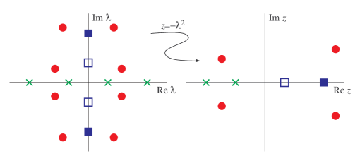
Figure 1: (color online) Six sets of eigenvalues and their images under the map. The (red) circles denote two quads of complex eigenvalues under the four-fold symmetry $\{\pm\lambda,\pm\overline{\lambda}\}$ and their images, $k_{\mathrm{c}}=2$. The (green) crosses denote two pairs of real eigenvalues $\{\pm\lambda\}$ and their images on the negative real axis, $k_{\mathrm{r}}=2$. The (blue) boxes denote two pairs of purely imaginary eigenvalues $\{\pm\lambda\}$ and their images on the positive real axis. The filled square has a positive Krein signature, while the empty square has a negative Krein signature, so that $k_{\mathrm{i}}^{-}=1$.

2.2.   The Krein matrix

We now turn to the problem of constructing a meromorphic matrix-valued function, the Krein matrix, which has the property that it is singular precisely for those values of $z$ which correspond to nonzero eigenvalues for the pencil

$$(\mathcal{R}-z\mathcal{S})u=0$$ (2.11)

where $\mathcal{R},\mathcal{S}$ are defined in (2.7). The Krein matrix was introduced in [13], and the interested reader should consult that work for the details associated with the following discussion (also see [14, Section 3]). We construct the Krein matrix by projecting off the finite-dimensional negative space of the operator $\mathcal{S}$, which as we have already seen in (2.9) has dimension $K_{\mathrm{Ham}}$, and then using a Lyapunov-Schmidt reduction to compute an equivalent eigenvalue problem.

Let $N(\mathcal{S})$ denote the $K_{\mathrm{Ham}}$-dimensional negative subspace of $S$, and let $P:X\mapsto N(\mathcal{S})^{\perp}$ be the orthogonal projection. Define the constrained operators

$$\mathcal{R}_{2}\mathrel{\mathop{:}}=P\mathcal{R}P,\quad\mathcal{S}_{+}\mathrel{\mathop{:}}=P\mathcal{S}P.$$

The operator $\mathcal{S}_{+}$ is positive definite and symmetric, whereas from the Index Theorem [14, Theorem 2.1] the symmetric operator $\mathcal{R}_{2}$ satisfies

$$\mathrm{n}(\mathcal{R}_{2})=\mathrm{n}(\mathcal{R})-\mathrm{n}(\mathcal{R}^{-1}_{N(\mathcal{S})})=K_{\mathrm{Ham}}-\mathrm{n}(\mathcal{R}^{-1}_{N(\mathcal{S})}).$$

Since $\mathcal{S}_{+}$ is positive definite we can define the conjugated operator

$$\widetilde{\mathcal{R}}\mathrel{\mathop{:}}=\mathcal{S}_{+}^{-1/2}\mathcal{R}_{2}\mathcal{S}_{+}^{-1/2},$$

and note that the invertibility of $\mathcal{S}$ yields

$$\mathrm{n}(\widetilde{\mathcal{R}})=\mathrm{n}(\mathcal{R}_{2}).$$

Upon writing a potential eigenfunction to the linear pencil as

$$u=\sum_{j=1}^{K_{\mathrm{Ham}}}c_{j}s_{j}^{-}+s^{+},\quad s^{+}\in N(\mathcal{S})^{\perp},$$

where $\{s_{1},\dots,s_{K_{\mathrm{Ham}}}\}$ is an orthonormal spectral basis for $N(\mathcal{S})$, and applying the projection $P$ to (2.11), the pencil problem becomes

$$(\mathcal{R}_{2}-z\mathcal{S}_{2})s^{+}+\sum_{j=1}^{K_{\mathrm{Ham}}}c_{j}P\mathcal{R}s_{j}=0.$$

On the other hand, upon applying $Q=\mathcal{I}-P$ to (2.11), where $\mathcal{I}$ is the identity operator, and taking the inner product of the resulting equation with $s_{\ell}$ for $\ell=1,\dots,K_{\mathrm{Ham}}$, yields the system of equations

$$\langle\mathcal{R}s^{+},s_{\ell}\rangle+\sum_{j=1}^{K_{\mathrm{Ham}}}c_{j}\langle\mathcal{R}s_{j},s_{\ell}\rangle=c_{\ell}z\lambda_{\ell},$$

where $\mathcal{S}s_{\ell}=\lambda_{\ell}s_{\ell}$. Solving the first equation for $s^{+}$ and plugging this result into the second equation yields the problem

$$\bm{\mathit{K}}(z)\bm{\mathit{c}}=\bm{\mathit{0}},\quad\bm{\mathit{K}}(z)\mathrel{\mathop{:}}=\mathcal{R}_{N(\mathcal{S})}-z\mathcal{S}_{N(\mathcal{S})}-(\widetilde{\mathcal{R}}-z)^{-1}_{\mathcal{S}_{+}^{-1/2}P\mathcal{R}N(\mathcal{S})}.$$ (2.12)

Here we are using the notation

$$\mathcal{S}_{+}^{-1/2}P\mathcal{R}N(\mathcal{S})\mathrel{\mathop{:}}=\{\mathcal{S}_{+}^{-1/2}P\mathcal{R}s^{-}:s^{-}\in N(\mathcal{S})\}.$$

The matrix $\bm{\mathit{K}}(z)$ is known as the Krein matrix.

We now relate the properties of the problem (2.12) to those for the original pencil (2.11). By construction $z$ is an eigenvalue for the pencil (2.8) with corresponding eigenfunction $u$ if and only if $\bm{\mathit{K}}(z)\bm{\mathit{c}}=\bm{\mathit{0}}$, where $\bm{\mathit{c}}=(c_{1},\dots,c_{K_{\mathrm{Ham}}})^{\mathrm{T}}$. If for a particular eigenvalue $z$ it is true that $u\notin N(\mathcal{S})^{\perp}$, then it is necessarily true that $\mathop{\mathrm{missing}}{det}\nolimits\bm{\mathit{K}}(z)=0$. On the other hand, if $u\in N(\mathcal{S})^{\perp}$, then $\bm{\mathit{c}}=\bm{\mathit{0}}$, so it can be the case that $\mathop{\mathrm{missing}}{det}\nolimits\bm{\mathit{K}}(z)\neq 0$. Now, if $\mathop{\mathrm{missing}}{Im}\nolimits z\neq 0$, then it will always be the case that $z$ is an eigenvalue if and only if $\mathop{\mathrm{missing}}{det}\nolimits\bm{\mathit{K}}(z)=0$. On the other hand, if $z\in\mathbb{R}^{-}$ is an eigenvalue with $\mathop{\mathrm{missing}}{det}\nolimits\bm{\mathit{K}}(z)\neq 0$, then it is the case that for the Krein matrix constructed by projecting off of the negative directions of $\mathcal{R}$, say $\bm{\mathit{K}}_{\mathcal{R}}(z)$, we would necessarily have $\mathop{\mathrm{missing}}{det}\nolimits\bm{\mathit{K}}_{\mathcal{R}}(z)=0$. Finally, if $z\in\mathbb{R}^{+}$ is an eigenvalue with $\mathop{\mathrm{missing}}{det}\nolimits\bm{\mathit{K}}(z)\neq 0$, then the eigenvalue has positive Krein signature. In this case the eigenvalue is realized as a removable singularity of the Krein matrix, i.e., $z=z_{\mathrm{p}}$ is a pole of the Krein matrix for which the residue is the zero matrix. If the eigenvalue has negative Krein signature, it will necessarily be the case that $\mathop{\mathrm{missing}}{det}\nolimits\bm{\mathit{K}}(z)=0$.

In conclusion, we can use $\mathop{\mathrm{missing}}{det}\nolimits\bm{\mathit{K}}(z)$ as a meromorphic function whose zeros correspond to eigenvalues. The (potential) singularities of the Krein matrix arise through $(\widetilde{\mathcal{R}}-z)^{-1}_{\mathcal{S}_{+}^{-1/2}P\mathcal{R}N(\mathcal{S})}$ at the eigenvalues of the self-adjoint operator $\widetilde{\mathcal{R}}$. In order to use the Krein matrix to say something about the Krein signature of a real positive eigenvalue, it will be helpful to factor the determinant as a finite product. One can easily observe that $\bm{\mathit{K}}(z)$ is symmetric for all $z$, i.e., $\bm{\mathit{K}}(z)^{\mathrm{T}}=\bm{\mathit{K}}(z)$; in particular, it is Hermitian for $z\in\mathbb{R}$. This allows us for $z\in\mathbb{R}$ to extract the $K_{\mathrm{Ham}}$ eigenvalues of the Krein matrix, $r_{j}(z)$, hereafter called the Krein eigenvalues, in a meromorphic fashion. Thus, instead of finding eigenvalues by looking for the zeros of the determinant of the Krein matrix, we can look for the zeros of each individual Krein eigenvalue. There will be precisely $K_{\mathrm{Ham}}$ of these Krein eigenvalues.

Remark 2.0.

Although we will not pursue this line of thought herein, each Krein eigenvalue can be thought of as a real meromorphic analogue of the Evans function [1]. Both Krein eigenvalues and the Evans function detect eigenvalue for a linear eigenvalue problem through the zeros. Until recently the Evans function was constructed solely via a dynamical systems argument, which necessitated that the eigenvalue problem be essentially in one space variable. Since the Krein matrix is constructed via a functional analytic argument, the spatial dimension associated with the eigenvalue problem is not relevant.

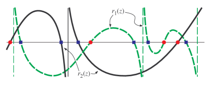
Figure 2: (color online) A cartoon of the graphs of the Krein eigenvalues for $z\in\mathbb{R}^{+}$ in the case that $K_{\mathrm{Ham}}=2$. The Krein eigenvalue $r_{1}(z)$ is denoted by a thick (green) dashed curve, and its vertical asymptotes are given by a thin (green) dashed curve. The Krein eigenvalue $r_{2}(z)$ is denoted by a thick (black) curve, and its vertical asymptotes are given by a thin (black) curve. The eigenvalues for the pencil (2.11) with positive Krein index are denoted by (blue) squares, and those with negative index are shown as (red) circles.

For real-valued $z$, the properties of the Krein eigenvalues are as follows. First,

$$\lim_{z\to-\infty}\frac{r_{j}(z)}{z}>0,$$

so that each Krein eigenvalue is negative for large negative $z$. This follows from the fact that $\mathcal{S}_{N(\mathcal{S})}$ is a negative definite matrix. Second, if $z_{\mathrm{p}}$ is a pole of the the Krein eigenvalue $r_{j}(z)$, it will then be the case that

$$\lim_{z\to z_{\mathrm{p}}^{\pm}}r_{j}(z)=\pm\infty.$$

Furthermore, if $z^{*}$ is a simple eigenvalue of $\widetilde{\mathcal{R}}$, so that $z^{*}$ is a pole of the Krein matrix, then it will be the case that $z^{*}$ is a simple pole for only one of the Krein eigenvalues. In other words, for all but one of the Krein eigenvalues the pole $z^{*}$ of the Krein matrix is a removable singularity. Finally, if $z_{0}$ is a simple positive zero of the Krein eigenvalue $r_{j}(z)$, then it is true that

$$k^{-}_{\mathrm{i}}(z_{0})=-\mathop{\mathrm{missing}}{sign}\nolimits[r_{j}^{\prime}(z_{0})];$$

in other words, the slope of the Krein eigenvalue at a zero gives definitive information regarding the Krein index of the eigenvalue. This is the most useful of the properties of the Krein eigenvalues, for it allows us graphically locate those eigenvalues which have negative Krein signature. This discussion is summarized in Figure 2.

Remark 2.0.

If the zero of a Krein eigenvalue is not simple, then for the eigenvalue in question there will be an associated Jordan chain which has length equal to the order of the zero. Furthermore, this situation can only arise upon the collision of an (almost) equal number of purely imaginary eigenvalues with positive and negative Krein signature (see [13, Section 2.2] for the details).

2.3.   Summarizing remarks

Following subsection 2.1 we know that for the original eigenvalue problem (2.1) the Hamiltonian-Krein index is

$$\left(k_{\mathrm{r}}+2k_{\mathrm{c}}+2k_{\mathrm{i}}^{-}\right)(\lambda)=K_{\mathrm{Ham}},$$

while for the pencil (2.11) the index is

$$\left(k_{\mathrm{r}}+2k_{\mathrm{c}}+2k_{\mathrm{i}}^{-}\right)(z)=2K_{\mathrm{Ham}}.$$

The individual indices are related via

$$k_{\mathrm{r}}(z)=2k_{\mathrm{r}}(\lambda),\quad k_{\mathrm{c}}(z)=2k_{\mathrm{c}}(\lambda),\quad k_{\mathrm{i}}^{-}(z)=2k_{\mathrm{i}}^{-}(\lambda).$$

For the original eigenvalue problem there will be an infinite number of purely imaginary eigenvalues, all of which but a finite number will have positive Krein index. The purely imaginary eigenvalues with negative Krein signature can be determined by first constructing the Krein matrix of (2.12) for the pencil (2.11), and then plotting the resultant Krein eigenvalues for $z\in\mathbb{R}$. In particular, the eigenvalues with negative signature will correspond to those values of $z\in\mathbb{R}$ such that for some $1\leq j\leq K_{\mathrm{Ham}}$,

$$r_{j}(z)=0,\quad r_{j}^{\prime}(z)>0.$$

If the order of a zero of a Krein eigenvalue is two or higher, then a collision of eigenvalues of opposite Krein signature has occurred.

Remark 2.0.

The discussion in this section assumed that the original Hamiltonian eigenvalue problem is not in the canonical form of subsection 2.1. If the problem is in canonical form, adjustments must be made: this is discussed in the application presented in section 4.

3.   Application: spectral analysis for vortices of the GP equation

We now wish to use the Krein matrix to identify the eigenvalues of (2.1) which have nonzero real part, or which are purely imaginary and have negative Krein signature. We intend to explore these spectral features and confirm them against a full linear stability analysis for an example of significant interest to recent experimental applications, namely the study of a single vortex [6] and of a pair of vortices [28, 27] in two-dimensional Bose-Einstein condensates as described by the GP Equation. The Hamiltonian-Krein index of (2.10) tells us how many of these zeros for the pencil we need to find in order to fully capture all of the (potentially) unstable eigenvalues. The real eigenvalues for the linearized problem correspond to negative real eigenvalues for the pencil, and the eigenvalues with nonzero real part correspond to eigenvalues with nonzero imaginary part for the pencil. Regarding the eigenvalues with negative signature, from the discussion of the previous section this means that we need to identify the real and positive eigenvalues for the pencil (2.8) for which a Krein eigenvalue has a zero, and the slope of the curve at the zero is positive.

The model under consideration for the case of pancake-shaped Bose-Einstein condensates [21, 6, 27] is the (2+1)-dimensional Gross-Pitaevskii equation in the dimensionless form

$$\mathrm{i}\partial_{t}u=-\frac{1}{2}\Delta u+V(x,y)u+|u|^{2}u-\mu u.$$ (3.1)

Here, $u$ is the macroscopic wave function, $V(x,y)=\Omega^{2}\left(x^{2}+y^{2}\right)/2$ is the external harmonic potential, $\Omega$ is the frequency of the trap, $\mu$ is the chemical potential, and $\Delta$ is the Laplace operator, i.e., $\Delta=\partial_{xx}+\partial_{yy}$. For the problem discussed herein, we assume $\Omega=0.2$.

We begin by assuming that the steady-state problem is solved, and we will denote that solution by $u_{0}(x,y)=U_{0}(x,y)+\mathrm{i}V_{0}(x,y)$. Here $U_{0},V_{0}$ are real-valued functions. Writing

$$U_{0}(x,y)+\mathrm{i}V_{0}(x,y)=\rho(r,\theta)\mathrm{e}^{\mathrm{i}\phi(r,\theta)},\quad\tan\theta=y/x,$$

where $r^{2}=x^{2}+y^{2}$, the wave will have the property that $\rho(r,\theta)\to 0$ exponentially fast as $r\to+\infty$. As for the associated eigenvalue problem, abusing notation a bit and writing

$$u\mapsto U_{0}+\mathrm{i}V_{0}+\epsilon(u+\mathrm{i}v),\quad 0<\epsilon\ll 1,$$

we see that at $\mathcal{O}(\epsilon)$ we have the linear problem

$$\partial_{t}\bm{\mathit{u}}=\mathcal{J}\mathcal{L}\bm{\mathit{u}},\quad\bm{\mathit{u}}=(u,v)^{\mathrm{T}},$$

where

$$\mathcal{J}=\left(\begin{array}[]{rr}0&1\\ -1&0\end{array}\right),\quad\mathcal{L}=\left(\begin{array}[]{cc}-\frac{1}{2}\Delta-\mu+V(r)+3U_{0}^{2}+V_{0}^{2}&2U_{0}V_{0}\\ 2U_{0}V_{0}&-\frac{1}{2}\Delta-\mu+V(r)+U_{0}^{2}+3V_{0}^{2}\end{array}\right).$$

The eigenvalue problem of the form (2.1), i.e.,

$$\mathcal{J}\mathcal{L}\bm{\mathit{u}}=\lambda\bm{\mathit{u}},$$ (3.2)

arises upon using the separation of variables ansatz $\bm{\mathit{u}}\mapsto\bm{\mathit{u}}\mathrm{e}^{\lambda t}$.

With respect to the standard inner-product on $L^{2}(\mathbb{R}^{2})\times L^{2}(\mathbb{R}^{2})$ the operator $\mathcal{J}$ is boundedly invertible and skew-symmetric, while the operator $\mathcal{L}$ is self-adjoint. Furthermore, since the potential $V(r)$ grows quadratically, and the magnitude of the solution $|u_{0}(x,y)|=\rho(r,\theta)$ decays exponentially fast as $r\to+\infty$, it is the case that $\mathcal{L}$ has a compact resolvent. In order to construct the Krein matrix for the spectral problem we first follow (2.5) and set

$$\mathcal{L}_{+}=\mathcal{L},\quad\mathcal{L}_{-}=-\mathcal{J}\mathcal{L}\mathcal{J}.$$

The construction of the Krein matrix requires that we consider the spectral problem on the space perpendicular to the kernel of both operators. The fact that solutions to (3.1) are invariant under $u(x,y)\mapsto u(x,y)\mathrm{e}^{\mathrm{i}\phi}$ and the spatial rotation $u(x,y)\mapsto u(x\cos\theta-y\sin\theta,x\sin\theta+y\cos\theta)$ means that (generically) the kernel of $\mathcal{L}$ will be two-dimensional, so that (generically)

$$\begin{split}\mathop{\mathrm{missing}}{ker}\nolimits(\mathcal{L})=\mathop{\mathrm{missing}}{ker}\nolimits(\mathcal{L}_{+})&=\mathop{\mathrm{missing}}{span}\nolimits\{\left(\begin{array}[]{r}-V_{0}\\ U_{0}\end{array}\right),\left(\begin{array}[]{c}(\partial_{\theta}\rho)\cos\phi-(\partial_{\theta}\phi)V_{0}\\ (\partial_{\theta}\rho)\sin\phi+(\partial_{\theta}\phi)U_{0}\end{array}\right)\}\\ \mathop{\mathrm{missing}}{ker}\nolimits(-\mathcal{J}\mathcal{L}\mathcal{J})=\mathop{\mathrm{missing}}{ker}\nolimits(\mathcal{L}_{-})&=\mathop{\mathrm{missing}}{span}\nolimits\{\left(\begin{array}[]{c}U_{0}\\ V_{0}\end{array}\right),\left(\begin{array}[]{r}(\partial_{\theta}\rho)\sin\phi+(\partial_{\theta}\phi)U_{0}\\ -(\partial_{\theta}\rho)\cos\phi+(\partial_{\theta}\phi)V_{0}\end{array}\right)\}.\end{split}$$ (3.3)

If the solution has a radially symmetric density, i.e., $\rho=\rho(r)$, then the dimension of each kernel is (generically) one with

$$\mathop{\mathrm{missing}}{ker}\nolimits(\mathcal{L}_{+})=\mathop{\mathrm{missing}}{span}\nolimits\{\left(\begin{array}[]{r}-V_{0}\\ U_{0}\end{array}\right)\},\quad\mathop{\mathrm{missing}}{ker}\nolimits(\mathcal{L}_{-})=\mathop{\mathrm{missing}}{span}\nolimits\{\left(\begin{array}[]{c}U_{0}\\ V_{0}\end{array}\right)\}.$$

With this information at hand, and setting $\Pi:L^{2}(\mathbb{R}^{2})\times L^{2}(\mathbb{R}^{2})\mapsto[\mathop{\mathrm{missing}}{ker}\nolimits(\mathcal{L}_{+})\oplus\mathop{\mathrm{missing}}{ker}\nolimits(\mathcal{L}_{-})]^{\perp}$ to the the orthogonal projection, we can now compute the restricted operators

$$\mathcal{R}=\Pi\mathcal{L}_{+}\Pi,\quad\mathcal{S}^{-1}=\Pi\mathcal{L}_{-}\Pi$$

to create the pencil

$$(\mathcal{R}-z\mathcal{S})\bm{\mathit{u}}=\bm{\mathit{0}},\quad z=-\lambda^{2}.$$

The Krein matrix $\bm{\mathit{K}}(z)\in\mathbb{C}^{\mathrm{n}(\mathcal{S})\times\mathrm{n}(\mathcal{S})}$ (see (2.12)) will be created from this pencil using the algorithm described in the previous section.

3.1.   Single vortex state

Here we assume that the solution is a vortex of charge one. The solution is of the form

$$u_{0}(x,y)=\rho(r)\mathrm{e}^{\mathrm{i}\theta},$$

where the density profile satisfies $\rho(0)=0$, and the phase rotates by $2\pi$ around the vortex core, justifying the topological charge of the structure [21, 22]. The density and phase profiles for the single vortex state are shown in Figure 3, and the corresponding linearization spectrum is shown in Figure 4. The absolute value of this configuration is radially symmetric (a feature not shared by the vortex dipole state considered below), while its decay for $r\rightarrow\infty$ is dictated by the underlying linear problem being exponential for small $\mu$ [19] and resembling an inverted parabola for large $\mu$ [31] (the latter decay features are also shared by the vortex dipoles below). The dependence of the relevant eigenvalues as a function of the canonical parameter of the system, namely the chemical potential $\mu$ associated with the number of atoms in the condensate, has been quantified previously; see e.g. [22, 26]. We will confirm these findings via the Krein matrix, and showcase particular examples for a few representative values of $\mu$.

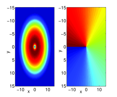
Figure 3: (color online) The single vortex state for a trap strength $\Omega=0.2$ and chemical potential $\mu=3$. The left panel shows the contour plot of the density, and the right panel is the phase plot for the wave function. In this case, the total number of grid points is $n=120$, and the spatial step size is $\Delta x=0.25$.

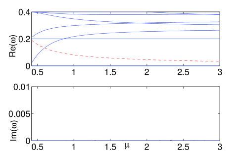
Figure 4: (color online) The real and imaginary parts of the eigenfrequencies defined by $\omega=\mathrm{i}\lambda$ for vortex dipole state when $n=120$ and $\Delta x=0.25$ as a function of the chemical potential $\mu$. Since the (red) dashed curve emanating from $\omega=0.2$ corresponds to an eigenvalue with negative Krein signature, the fact that $K_{\mathrm{Ham}}=2$ means that there are no other eigenvalues with positive real part (see (3.5)). The wave is spectrally stable for all considered values of the chemical potential. The eigenvalue which has negative Krein signature is highlighted as the (red) dashed line. Larger (in magnitude) eigenvalues along the imaginary axis have a positive Krein signature and do not lead to instabilities.

As we saw above, the kernels of the operators $\mathcal{L}_{\pm}$ each have dimension one. For small amplitude vortices where the nonlinear interactions are (almost) negligible it can be shown via an analysis similar to that presented in [19] that the Hamiltonian-Krein index satisfies $K_{\mathrm{Ham}}=2$. Following the discussion in subsection 2.3 we then know that for the pencil

$$\left(k_{\mathrm{r}}+2k_{\mathrm{c}}+2k_{\mathrm{i}}^{-}\right)(z)=4,$$ (3.4)

while for the original problem

$$\left(k_{\mathrm{r}}+2k_{\mathrm{c}}+2k_{\mathrm{i}}^{-}\right)(\lambda)=2.$$ (3.5)

Thus, if for the pencil there are two positive real zeros of the Krein eigenvalues which correspond to an eigenvalue with negative Krein index, the rest of the spectrum for the pencil must be positive and purely real. In other words, if for the original eigenvalue problem there is a purely imaginary eigenvalue with negative Krein index, the rest of the spectrum must be purely imaginary with positive Krein index. Consequently, once we numerically find one purely imaginary eigenvalue with negative Krein signature, or one set of eigenvalues with nonzero real part which satisfy the Hamiltonian eigenvalue symmetry, we need not search for any additional unstable eigenvalues. They simply do not exist.

Regarding the numerical solution and analysis of the problem, we first discretize the differential operator via a centered finite difference scheme using $n$ data points and a spatial interval of $\Delta x$. The single vortex state - indeed, any stationary solution - is found by applying Newton’s method to the discretized problem, treating it as a two-dimensional boundary value problem and starting from a suitably proximal to it initial guess. As for the spectral problem, the smallest (in norm) eigenvalues are computed using the MATLAB function “eigs” on the discretized version of the operator $\mathcal{J}\mathcal{L}$; i.e., we construct the linearization operator on the same domain as used for the fixed point iteration and utilize standard routines (such as an implicitly restarted Arnoldi method within MATLAB) to compute some of the smallest magnitude eigenvalues of the corresponding spectral problem. This provides us with the linear stability results that will be compared with the Krein matrix ones in the figures that follow. It is worth noting here that these spectral linearization results can only be obtained by taking advantage of the sparse structure of the underlying discretization matrix. Should the full eigenvalue spectrum of the linearization problem be sought in this highly-demanding two-dimensional computation, MATLAB’s routine “eig” would have been unable to produce the corresponding numerical results.

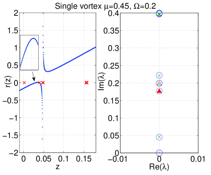
Figure 5: (color online) The numerically generated spectral plot for $n=48,\,\mu=0.45,\,\Delta x=0.45$. In the left panel the left plot is the numerically generated plot of the $K_{\mathrm{Ham}}=2$ Krein eigenvalues. For this problem the Krein matrix is a meromorphic multiple of the identity; hence, the two Krein eigenvalues coincide. The (red) crosses are the poles of the Krein matrix. If the pole is removable (e.g., for $z\sim 0.155$), then it corresponds to an eigenvalue with positive Krein signature. Here we see two positive real zeros of the Krein eigenvalues for which the functions have positive slope. Thus, for the pencil $k_{\mathrm{i}}^{-}(z)=2$ with $k_{\mathrm{r}}(z)=k_{\mathrm{c}}(z)=0$, which means that for the original problem (3.2) $k_{\mathrm{i}}^{-}(\lambda)=1$ with $k_{\mathrm{r}}(\lambda)=k_{\mathrm{c}}(\lambda)=0$. The wave is spectrally stable, but is not a (local) minimizer for the constrained Hamiltonian. In the right figure the eigenvalues for $\mathcal{J}\mathcal{L}$ are denoted by (blue) circles. The (green) crosses represent the poles of the Krein matrix, and the (red) triangles are the eigenvalues of $\mathcal{J}\mathcal{L}$ which are realized as zeros of the Krein eigenvalues. The purely imaginary eigenvalue with negative Krein signature is shown as a filled (red) triangle.

We now turn to a direct comparison of the numerical results for eigenvalues obtained from the linear stability analysis (which has partially been presented in earlier publications, see e.g. [26]) and from the Krein matrix, presented for the first time for vortex patterns of the GP equation herein. Here, we have confirmed the above findings with $\mu=0.45$ in Figure 5, and $\mu=0.75$ in Figure 6. In both of these figures a spatial discretization spacing of $\Delta x=0.5$ was used. Similar results were found with smaller values of $\Delta x$. In the right panel of each figure the spectrum of $\mathcal{J}\mathcal{L}$ was computed for both the original formulation of (3.2) and the corresponding pencil formulation (2.8), and the results of the two were found to agree within the accuracy of the eigenvalue solver. These spectral results were then compared with the prediction of the Krein matrix in the right panel. The agreement is excellent.

Unexpectedly, it turns out to be the case that for the problem at hand the Krein matrix is a meromorphic multiple of the identity; hence, the two Krein eigenvalues coincide. In both figures it is clear that there are then two zeros of the Krein eigenvalues at which the slope of the curve is positive: this corresponds to an purely imaginary eigenvalue with negative Krein signature. As stipulated by Hamiltonian-Krein index in (3.6), the rest of the spectrum must be purely imaginary, and this is indeed seen to be the case.

For the spectrum there is not only the eigenvalue at $\lambda=0$ which is due to the phase U$(1)$ gauge invariance of the model, there is also a double eigenvalue at $\lambda=\pm 0.2\mathrm{i}$. The latter frequency of double multiplicity is the so-called dipolar mode of the condensate and pertains to a symmetry (oscillation of the entire condensate cloud in the $x-$ or $y-$ direction with the trap frequency), and is hence invariant with respect to variations in $\mu$. One of these modes pertains to a pole of the Krein matrix, while the other is a zero of a Krein eigenvalue. The eigenvalue with negative Krein signature always lies between the origin and this double pair and is known to tend to the origin as the chemical potential $\mu$ increases [26, 22]. Since the eigenvalue has negative signature, as predicted by the theory it is realized as a zero of a Krein eigenvalue.

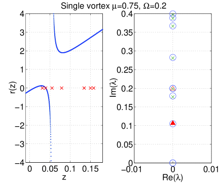
Figure 6: (color online) The numerically generated spectral plot for $n=48,\,\mu=0.75,\,\mathrm{d}x=0.45$. In the left panel the left plot is the numerically generated plot of the $K_{\mathrm{Ham}}=2$ Krein eigenvalues. For this problem the Krein matrix is a meromorphic multiple of the identity; hence, the two Krein eigenvalues coincide. The (red) crosses are the poles of the Krein matrix, and the removable singularities (e.g., $z\sim 0.08$) correspond to eigenvalues with positive Krein signature. Here we again see two positive real zeros of the Krein eigenvalues for which the functions have positive slope. The wave is then spectrally stable with $k_{\mathrm{i}}^{-}(\lambda)=1$ for the problem (3.2). The notation used in the right figure is similar to that in Figure 5.

To showcase the relevance of this pole, the residues of the poles of the Krein matrix are computed. If the numerically computed residue of the pole is of $\mathcal{O}(10^{-12})$, then we say that the pole is removable, and hence it corresponds to an eigenvalue with positive Krein signature. The residue is computed via the numerical integration

$$\mathop{\mathrm{missing}}{Res}\limits(\bm{\mathit{K}}(z),z_{\mathrm{p}})=\frac{1}{2\pi\mathrm{i}}\oint_{C}\bm{\mathit{K}}(z)\,\mathrm{d}z\sim\frac{1}{2\pi\mathrm{i}}\sum_{i=1}^{n}\bm{\mathit{K}}(z_{\mathrm{p},i})\Delta z_{\mathrm{p},i}.$$

Here $z_{\mathrm{p}}$ is the relevant pole of the Krein matrix, $n$ is the number of integration points on the simple positively oriented closed contour $C$ which surrounds the pole (here the contour is without loss of generality chosen to be a square centered on the pole), $z_{\mathrm{p},i}$ is the point on the integration contour around the pole, and $\Delta z_{\mathrm{p},i}$ is the segment on the integration path.

When the chemical potential $\mu=0.45$ the first relevant pole we choose is located at $z_{\mathrm{p}}=0.0021$. For the increment of $|\Delta z_{\mathrm{p},i}|=5*10^{-6}$ it is seen that

$$\oint_{C}\bm{\mathit{K}}(z)\,\mathrm{d}z=\left(\begin{array}[]{ccc}-8.4*10^{-12}-\mathrm{i}2.1*10^{-14}&-4.5*10^{-22}-\mathrm{i}9.5*10^{-20}\\ -2.8*10^{-21}-\mathrm{i}1.1*10^{-19}&-8.4*10^{-12}-\mathrm{i}2.1*10^{-14}\end{array}\right),$$

so that $|\mathop{\mathrm{missing}}{Res}\limits(\bm{\mathit{K}}(z),0.0021)|=\mathcal{O}(10^{-12})$. The simple pole is removable, and corresponds to a purely imaginary eigenvalue (the first red cross above zero in Figure 5). The fact that the singularity is removable is evidenced by the fact that neither of the Krein eigenvalues has a singularity at the point. Now consider the pole at $z_{\mathrm{p}}=0.0478$. It is seen that

$$\oint_{C}\bm{\mathit{K}}(z)\,\mathrm{d}z=\left(\begin{array}[]{ccc}-\mathrm{i}0.0057&-8.6*10^{-18}-\mathrm{i}3.0*10^{-15}\\ -5.5*10^{-18}-\mathrm{i}2.2*10^{-15}&-\mathrm{i}0.0057\end{array}\right),$$

so that $|\mathop{\mathrm{missing}}{Res}\limits(\bm{\mathit{K}}(z),0.0478)|=\mathcal{O}(10^{-3})$, which is nonzero by our criterion. Alternatively, we see that the pole is not removable because the Krein eigenvalues have a singularity at that point. Since the singularity is not removable, this point does not correspond to an eigenvalue.

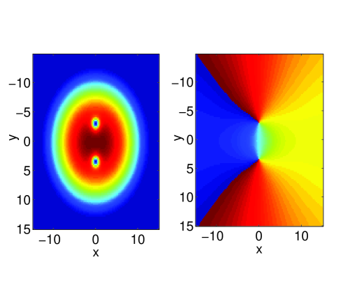
Figure 7: (color online) The vortex dipole state for a trap strength $\Omega=0.2$ and chemical potential $\mu=3$. The left panel shows the contour plot of the density, and the right panel is the phase plot for the wave function. In this case, the total number of grid points is $n=120$, and the spatial step size is $\mathrm{d}x=0.25$.

3.2.   Vortex dipole state

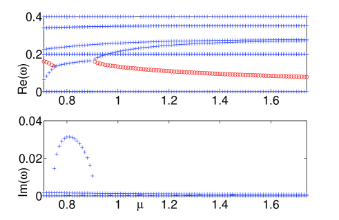
Figure 8: (color online) The real and imaginary parts of the eigenfrequencies defined by $\omega=\mathrm{i}\lambda$ for vortex dipole state when $n=480$ and $\mathrm{d}x=0.0625$ as a function of the chemical potential $\mu$. The wave is spectrally unstable with $k_{\mathrm{c}}(\lambda)=1,\,(k_{\mathrm{c}}(z)=2)$ when $\mathop{\mathrm{missing}}{Im}\nolimits\omega>0$. When $k_{\mathrm{c}}(\lambda)=1$ we know by the Hamiltonian-Krein index for the wave that there are no other unstable eigenvalues. When $k_{\mathrm{c}}(\lambda)=k_{\mathrm{r}}(\lambda)=0$ in the figure, the eigenvalue associated with (red) circles has negative Krein signature. By the Hamiltonian-Krein index we then know that there are no other non-plotted eigenvalues with positive real part, so that in this case the wave is spectrally stable.

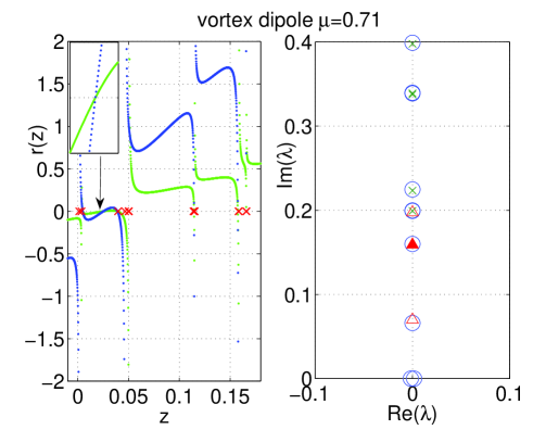
Figure 9: (color online) The numerically generated spectral plot for the vortex dipole when $\Omega=0.2$ and $\mu=0.71$. The left panel is the plot of the two Krein eigenvalues: the (red) crosses represent the poles of the Krein matrix, and the removable singularities correspond to eigenvalues with positive Krein signature. Note that $k_{\mathrm{i}}^{-}(z)=2$ for the pencil, and that as expected the zeros of the Krein eigenvalues which correspond to eigenvalues with negative Krein signature coincide. In the right panel the (blue) circles are the eigenvalues for $\mathcal{J}\mathcal{L}$, the (red) triangles are the eigenvalues which correspond to zeros of the Krein eigenvalues, and the (green) crosses are the eigenvalues which correspond to removable singularities of the Krein matrix - these eigenvalues have positive Krein signature. The purely imaginary eigenvalue with negative Krein signature is shown as a filled (red) triangle. The labeling of eigenvalues in the right panel is the same as for Figure 5.

We now turn to a spectral analysis for the vortex dipole state, which is a stationary vortex-antivortex state (see Figure 7 for a typical example of its density and phase). When $\Omega=0.2$ the vortex dipole state exists for $\mu>0.68$. It is interesting to note here that, as shown in [24, 26], such states do not exist at the linear limit, but only bifurcate through a supercritical pitchfork (symmetry-breaking) event at a critical point from the dark soliton, which corresponds to the real-valued (first) excited state of the two-dimensional harmonic oscillator. Since the density is not radially symmetric, it will (generically) be the case that $\mathop{\mathrm{missing}}{dim}\nolimits[\mathop{\mathrm{missing}}{ker}\nolimits(\mathcal{L}_{\pm})]=2$. Furthermore, it is seen numerically that $\mathrm{n}(\mathcal{S})=K_{\mathrm{Ham}}=2$, so that by subsection 2.1 we have the same index count for the pencil as (3.6); namely,

$$\left(k_{\mathrm{r}}+2k_{\mathrm{c}}+2k_{\mathrm{i}}^{-}\right)(z)=4\quad\Leftrightarrow\quad\left(k_{\mathrm{r}}+2k_{\mathrm{c}}+2k_{\mathrm{i}}^{-}\right)(\lambda)=2.$$ (3.6)

As in the previous example, there will be two Krein eigenvalues to be plotted. Unlike the previous example, the Krein matrix will not be a meromorphic multiple of the identity; hence, the Krein eigenvalues will not generically overlap. If there are two positive real zeros of the Krein eigenvalues for which the curves have positive slope, then the spectrum for the pencil will be positive and purely real with $k_{\mathrm{i}}^{-}(z)=2\,(k_{\mathrm{i}}^{-}(\lambda)=1)$. Otherwise the underlying wave will be unstable. As we will see, in our examples this instability will arise when $k_{\mathrm{c}}(z)=2\,(k_{\mathrm{c}}(\lambda)=1)$. It is important to note here that for the pencil it must be the case that if $k_{\mathrm{i}}^{-}(z)=2$, then each Krein eigenvalue has a positive zero at precisely the same point. This fact is a consequence of the relationship of the spectrum between the original eigenvalue problem and the pencil; in particular, the fact that the spectrum of the pencil “doubles up” the nonzero spectrum for the original problem.

Figure 10: (color online) The numerically generated spectral plot for the vortex dipole when $\Omega=0.2$ and $\mu=0.80$. The left panel is the plot of the two Krein eigenvalues: the (red) crosses represent the poles of the Krein matrix, and the removable singularities correspond to eigenvalues with positive Krein signature. Since there are no positive real zeros with positive slope, it must be the case that for the pencil $k_{\mathrm{c}}(z)=2$. In the right panel the (blue) circles are the eigenvalues for $\mathcal{J}\mathcal{L}$, the (red) triangles are the eigenvalues which correspond to zeros of the Krein eigenvalues, and the (green) crosses are the eigenvalues which correspond to removable singularities of the Krein matrix - these eigenvalues have positive Krein signature. The labeling of eigenvalues in the right panel is the same as for Figure 5. The only difference is that the (blue) stars represent the complex eigenvalues with nonzero real part as found by the zeros of the Krein eigenvalues.

The spectrum once again features the twofold degenerate dipolar modes which are associated with the oscillation with the trap frequency of the whole condensate in the $x-$ and $y-$ directions. In addition to these modes, there exists a negative Krein signature mode, which in this case collides with the mode departing from zero. This, in turn, leads to the formation of an interval of $\mu$-values where the spectrum possesses complex eigenfrequencies associated with oscillatory instability. Therefore, when studying the computation of the Krein matrix of the vortex dipole state and comparing its eigenvalues against the linearization analysis, we select two cases, namely $\mu=0.71$ and $\mu=0.80$. As we see in Figure 8, the former is before the collision of the two modes (i.e., $k_{\mathrm{c}}(\lambda)=0$), and the latter is after the collision has occurred (i.e., $k_{\mathrm{c}}(\lambda)=1$). For larger values of $\mu$ the complex-valued eigenvalues return to the imaginary axis.

When $\mu=0.71$ we show the computation of the Krein eigenvalues (left panel) and the linearization spectrum (right panel) in Figure 9. In the right panel it can be observed that the zeros of the Krein eigenvalues are consistent with the eigenvalues found via the linear stability analysis, except for the real eigenvalues, which are $\mathcal{O}(10^{-3})$ and are the numerical approximation of the known zero eigenvalues. Regarding the left panel it is seen from the inset that $k_{\mathrm{i}}^{-}(z)\geq 2$. From (3.6) we know that the Hamiltonian-Krein index for the pencil is

$$\left(k_{\mathrm{r}}+2k_{\mathrm{c}}+2k_{\mathrm{i}}^{-}\right)(z)=4;$$

hence, for the pencil it is the case that $k_{\mathrm{i}}^{-}(z)=2$ with $k_{\mathrm{r}}(z)=k_{\mathrm{c}}(z)=0$. For the original problem it is then true that $k_{\mathrm{i}}^{-}(\lambda)=1$ with $k_{\mathrm{r}}(\lambda)=k_{\mathrm{c}}(\lambda)=0$. The eigenvalue with negative Krein signature is denoted by a (red) filled triangle in the right panel. As a consequence of the index theory we know that all other eigenvalues must be purely imaginary with positive Krein signature.

When $\mu=0.80$ we show the computation of the Krein eigenvalues (left panel) and the linearization spectrum (right panel) in Figure 10. Again, the zeros of the Krein eigenvalues are consistent with the eigenvalues found via the linear stability analysis except for the real eigenvalues, which are $\mathcal{O}(10^{-3})$ and are the numerical approximation of the known zero eigenvalues. From the right panel we see that $k_{\mathrm{c}}(\lambda)\geq 1$. Upon using (3.6) we then have that $k_{\mathrm{c}}(\lambda)=1\,(k_{\mathrm{c}}(z)=2)$ with $k_{\mathrm{r}}(\lambda)=k_{\mathrm{i}}^{-}(\lambda)=0$. As we see in the left panel, as expected the Krein eigenvalues have no negative zeros, and no positive zeros with positive slope; in other words, all of the zeros of the Krein eigenvalues correspond to purely imaginary eigenvalues with positive Krein signature. In conclusion, as a consequence of the index theory we know that except for the one quartet of simple eigenvalues with nonzero real and imaginary parts, all other eigenvalues must be purely imaginary with positive Krein signature. The unstable eigenvalues cannot be detected via the graph of the Krein eigenvalues in the left panel of Figure 10. However, they can be found by providing a phase plot for each Krein eigenvalue, which is done in Figure 11 when $\mu=0.80$. The axes denote the complex $z$-plane, and the colorbar corresponds to the phase of the eigenvalues of the Krein matrix. The points where the phase becomes singular correspond to the location of the complex eigenvalues, and are labeled by the white spots. It is clear from a standard winding number argument that each zero of the Krein eigenvalue is simple, which is a verification of the fact that $k_{\mathrm{c}}(z)=2$.

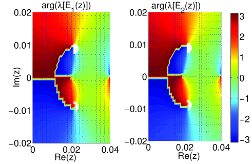
Figure 11: (color online) Phase plot for the Krein eigenvalues when $\mu=0.80$. The colors represent the argument of the Krein eigenvalues, $\mathop{\mathrm{missing}}{arg}\nolimits(\lambda(E_{1}(z)))$ and $\mathop{\mathrm{missing}}{arg}\nolimits(\lambda(E_{2}(z)))$. The two white spots on each of the two panels represent the complex eigenvalues, corresponding to $z=0.021\pm\mathrm{i}0.09$.

4.   Application: spectral analysis for multi-solitons of the GP equation

The model under consideration is the (1+1)-dimensional Gross-Pitaevskii equation in the dimensionless form

$$\mathrm{i}\partial_{t}u=-\frac{1}{2}\partial_{xx}u+V(x)u+|u|^{2}u-\mu u,$$ (4.1)

where now $V(x)=\Omega^{2}x^{2}/2$ is the external harmonic potential. When doing numerical computations for this problem we assume $\Omega=1$. For this problem we are interested in studying the spectrum associated with real-valued solutions. These will be denoted by $U_{0}(x)$, and they will be realized as solutions of the ODE

$$-\frac{1}{2}\partial_{xx}U_{0}+V(x)U_{0}+U_{0}^{3}-\mu U_{0}=0.$$

The solutions will have the property that $U_{0}(x)\to 0$ exponentially fast as $|x|\to+\infty$.

The eigenvalue problem associated with the real-valued solution will be exactly that as given in (3.2), except that now $\mathcal{L}$ will be diagonal, i.e., $\mathcal{L}=\mathop{\mathrm{missing}}{diag}\nolimits(\mathcal{L}_{+},\mathcal{L}_{-})$, with

$$\mathcal{L}_{+}=-\frac{1}{2}\partial_{x}^{2}-\mu+V(x)+3U_{0}^{2},\quad\mathcal{L}_{-}=-\frac{1}{2}\partial_{x}^{2}-\mu+V(x)+U_{0}^{2}.$$

The fact that $\mathcal{L}$ is diagonal, i.e., the eigenvalue problem is in the canonical form

$$\mathcal{L}_{+}u=-\lambda v,\quad\mathcal{L}_{-}v=\lambda u,$$

means that not only can more be said about the Hamiltonian-Krein index for the original problem, but the index for the associated pencil will also change. This latter amendment follows from the fact that the pencil can be formed directly without first passing to the intermediate stage of “doubling-up” the eigenvalue problem.

Because the operators $\mathcal{L}_{\pm}$

1. are Sturmian (e.g., see [15, Chapter 2.3])

2. contain the unbounded potential $x^{2}$

3. contain a potential which decays exponentially fast as $|x|\to+\infty$,

the general properties of $\sigma(\mathcal{L}_{\pm})$ are well-understood:

1. $\sigma(\mathcal{L}_{\pm})\subset\mathbb{R}$ is composed solely of point eigenvalues

2. each eigenvalue is geometrically and algebraically simple.

The operator $\mathcal{L}_{+}$ will (generically) be invertible, while $\mathcal{L}_{-}U_{0}=0$ implies that $\mathop{\mathrm{missing}}{dim}\nolimits[\mathop{\mathrm{missing}}{ker}\nolimits(\mathcal{L}_{-})]=1$. If we let $\Pi:X\mapsto\mathop{\mathrm{missing}}{span}\nolimits\{U_{0}\}^{\perp}$ denote the orthogonal (spectral) projection, and set

$$\mathcal{R}=\Pi\mathcal{L}_{+}\Pi,\quad\mathcal{S}^{-1}=\Pi\mathcal{L}_{-}\Pi,$$

then the search for nonzero eigenvalues for the original problem is equivalent to finding the spectrum of the pencil

$$(\mathcal{R}-z\mathcal{S})u=0,\quad z=-\lambda^{2}\quad\Rightarrow\quad\mathcal{R}u=-\lambda v,\,\,\mathcal{S}^{-1}v=\lambda u.$$

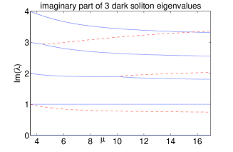
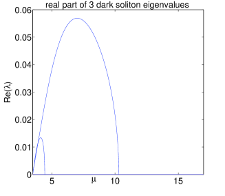
Figure 12: (color online) Linear stability analysis for the 3-dark-soliton states: left panel is $\mathop{\mathrm{missing}}{Im}\nolimits(\lambda)$ versus $\mu$, while the right panel is the $\mathop{\mathrm{missing}}{Re}\nolimits(\lambda)$ versus $\mu$. The first critical value of $\mu$ where one pair of the complex eigenvalues becomes purely imaginary is approximately $\mu=4.46$. The second critical value where the other pair of complex eigenvalues becomes purely imaginary is approximately $\mu=10.29$. The eigenvalue(s) which have negative Krein signature are shown as (red) dashed lines.

The Hamiltonian-Krein index for the original eigenvalue problem is given by

$$K_{\mathrm{Ham}}=\mathrm{n}(\mathcal{R})+\mathrm{n}(\mathcal{S})$$

(compare with (2.4)). Since $\Pi$ is a spectral projection, it will be the case that $\mathrm{n}(\mathcal{S})=\mathrm{n}(\mathcal{L}_{-})$. As for $\mathrm{n}(\mathcal{R})$, by using the Index Theorem in [13] it is the case that

$$\mathrm{n}(\mathcal{R})=\mathrm{n}(\mathcal{L}_{+})-\mathrm{n}(\langle U_{0},\mathcal{L}_{+}^{-1}U_{0}\rangle).$$

Upon using the fact that

$$\mathcal{L}_{+}(\partial_{\mu}U_{0})=U_{0}\quad\Rightarrow\quad\langle U_{0},\mathcal{L}_{+}^{-1}U_{0}\rangle=\frac{1}{2}\partial_{\mu}\langle U_{0},U_{0}\rangle$$

we have the rewritten expression

$$\mathrm{n}(\mathcal{R})=\mathrm{n}(\mathcal{L}_{+})-\mathrm{n}(\partial_{\mu}\langle U_{0},U_{0}\rangle).$$

In other words, the slope of the power curve $P(\mu)=\langle U_{0},U_{0}\rangle$ has a direct influence on the number of negative directions of the operator $\mathcal{L}_{+}$ (this is the so-called Vakhitov–Kolokolov stability criterion for canonical Hamiltonian eigenvalue problems). In conclusion, the Hamiltonian-Krein index for the canonical problem is

$$K_{\mathrm{Ham}}=\mathrm{n}(\mathcal{L}_{+})+\mathrm{n}(\mathcal{L}_{-})-\mathrm{n}(P^{\prime}(\mu)),\quad P(\mu)=\langle U_{0},U_{0}\rangle.$$ (4.2)

There is also an instability criterion. The classical result of Grillakis [7], Jones [12] (recently reproven in [14] using the Krein matrix) allows us to say that a lower bound on $k_{\mathrm{r}}(\lambda)$ is caused by a difference in the number of negative directions of $\mathcal{R}$ and $\mathcal{S}$. In other words,

$$k_{\mathrm{r}}(\lambda)\geq|\mathrm{n}(\mathcal{L}_{-})-[\mathrm{n}(\mathcal{L}_{+})-\mathrm{n}(P^{\prime}(\mu))]|,$$ (4.3)

which in particular implies the previously stated result that $k_{\mathrm{r}}(\lambda)\geq 1$ if $|\mathrm{n}(\mathcal{L}_{-})-\mathrm{n}(\mathcal{L}_{+})|\geq 2$.

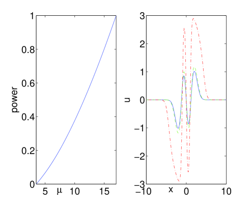
Figure 13: (color online) The left panel shows the power $P(\mu)$ (see (4.2)) versus the chemical potential $\mu$: the power plotted here is scaled by the $\max(P(\mu))$. The right panel demonstrates the stationary solutions as $\mu$ varies. The solid blue, dashed green, and dash-dotted red curves represent the cases of $\mu=4.2,4.6,10.3$ respectively. Here the grid size is $n=800$ and the spatial interval is $\Delta x=0.025$.

Regarding the Hamiltonian-Krein index for the pencil, the fact that the original system no longer needs to be “doubled-up” in order to be put into canonical form means that we just need to count eigenvalues with respect to the eigenvalue mapping $z=-\lambda^{2}$ (see Figure 1). In particular,

$$k_{\mathrm{r}}(\lambda)=k_{\mathrm{r}}(z),\quad k_{\mathrm{c}}(\lambda)=k_{\mathrm{c}}(z),\quad k_{\mathrm{i}}^{-}(\lambda)=k_{\mathrm{i}}^{-}(z),$$

which in the end means that the index for the pencil is precisely that for the original problem, and is given in (4.2). Additionally, in the construction of the Krein matrix the size no longer directly depends on $K_{\mathrm{Ham}}$; instead, it will be of size $\mathrm{n}(\mathcal{S})=\mathrm{n}(\mathcal{L}_{-})$.

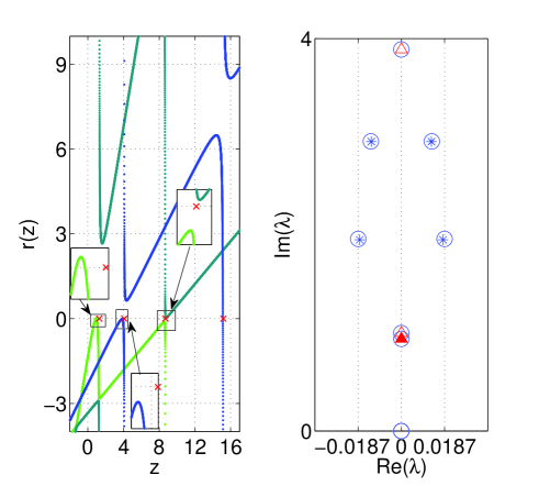
Figure 14: (color online) The spectral picture when $\mu=4.2$, for which $k_{\mathrm{c}}(\lambda)=2$ and $k_{\mathrm{i}}^{-}(\lambda)=1$. In the left panel is the plot of the three Krein eigenvalues. As predicted by the theory, there is only one positive zero of a Krein eigenvalue for which the slope is positive. In the right panel the eigenvalues for $\mathcal{J}\mathcal{L}$ are denoted by (blue) circles. The (red) triangles are the eigenvalues of $\mathcal{J}\mathcal{L}$ which are realized as zeros of the Krein eigenvalues. The (blue) stars represent the complex eigenvalues with nonzero real part as found by the zeros of the Krein eigenvalues. The eigenvalue with negative Krein signature is marked with a (red) filled triangle. Note that this eigenvalue is close to an eigenvalue with positive Krein signature, which implies that the system is close to a Hamiltonian-Hopf bifurcation point.

In the previous section we considered the spectral stability of solutions for which two Krein eigenvalues could be used to locate the spectrum. We now consider an example for which three Krein eigenvalues are needed. The steady-state solution $U_{0}$ to be considered, hereafter called a 3-dark-soliton, is realized as a continuation of the Gauss-Hermite function $(8x^{3}-12x)\mathrm{e}^{-x^{2}/2}$ from the chemical potential $\mu^{*}=3.5$ (recall that we assume $\Omega=1$). Let us first determine the Hamiltonian-Krein index associated with this solution. A weakly nonlinear analysis along the lines of that presented in, e.g., [16], shows that for $|\mu-\mu^{*}|$ small, the power satisfies the relationship $P^{\prime}(\mu)>0$ (the details are left for the interested reader). As we see from the numerics (see Figure 13), this relationship holds for all values of $\mu$ under consideration. Regarding the indices of the operators $\mathcal{L}_{\pm}$, the combination of $U_{0}$ having three zeros and Sturm-Liouville theory implies that $\mathrm{n}(\mathcal{L}_{-})=3$; consequently, in the Krein matrix analysis there will be three Krein eigenvalues to follow. Regarding the operator $\mathcal{L}_{+}$, it is the case that in the weakly nonlinear limit $\mathrm{n}(\mathcal{L}_{+})=3$: again, this relationship holds for all $\mu$ under consideration. Appealing to (4.2) we see that $K_{\mathrm{Ham}}=6$; unfortunately, the lower bound of (4.3) on $k_{\mathrm{r}}(\lambda)$ leads to no definitive conclusion. Regarding the types of (potentially) unstable eigenvalues, we have the following possibilities:

$k_{\mathrm{r}}(\lambda)$	0	0	0	0	2	2	2	4	4	6
$k_{\mathrm{c}}(\lambda)$	0	1	2	3	0	1	2	0	1	0
$k_{\mathrm{i}}^{-}(\lambda)$	3	2	1	0	2	1	0	1	0	0

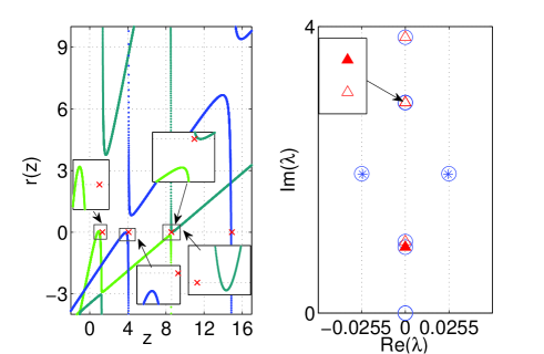
Figure 15: (color online) Similar to Figure 14, except now $\mu=4.46$ and $k_{\mathrm{c}}(\lambda)=1$ with $k_{\mathrm{i}}^{-}(\lambda)=2$.

In Figure 12 we show the location of the first few eigenvalues from the linear stability analysis as a function of $\mu$. It is always the case that $k_{\mathrm{r}}(\lambda)=0$, while $k_{\mathrm{c}}(\lambda)$ decreases from two to one to zero. The decreasing of $k_{\mathrm{c}}(\lambda)$ implies that $k_{\mathrm{i}}^{-}(\lambda)$ increases from one to two to three. The critical values of $\mu$ for which $k_{\mathrm{c}}(\lambda)$ decreases are approximately $\mu\sim 4.465$ and $\mu\sim 10.29$. In Figure 14 we show the plot of the Krein eigenvalues (left panel) and full linearization spectrum (right panel) when $\mu=4.2$, when $k_{\mathrm{c}}(\lambda)=2$ and $k_{\mathrm{i}}^{-}(\lambda)=1$. The eigenvalue in the upper half-plane with negative Krein signature is denoted with a (red) filled triangles. In Figure 15 we show the plot of the Krein eigenvalues (left panel) and full linearization spectrum (right panel) when $\mu=4.46$, when $k_{\mathrm{c}}(\lambda)=1$ and $k_{\mathrm{i}}^{-}(\lambda)=2$. The two eigenvalues in the upper half-plane with negative Krein signature are denoted with (red) filled triangles. Finally, in Figure 16 we show the plot of the Krein eigenvalues (left panel) and full linearization spectrum (right panel) when $\mu=10.30$, when $k_{\mathrm{i}}^{-}(\lambda)=3$. The three eigenvalues in the upper half-plane with negative Krein signature are denoted with (red) filled triangles.

Remark 4.0.

In general, when considering $N$-dark-solitons to (4.1) it will be the case that $P^{\prime}(\mu)>0$ with $\mathrm{n}(\mathcal{L}_{+})=\mathrm{n}(\mathcal{L}_{-})=N$. Consequently, when looking for the $2N$ (potentially) unstable eigenvalues for the linearized problem it will be the case that $N$ Krein eigenvalues must be plotted.

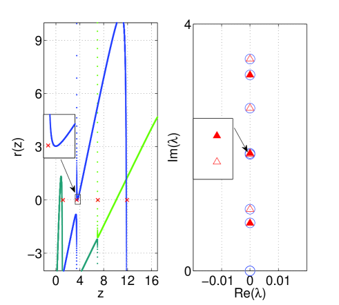
Figure 16: (color online) Similar to Figure 14, except now $\mu=10.30$ and $k_{\mathrm{i}}^{-}(\lambda)=3$.

5.   Conclusion

In the present work we have revisited Hamiltonian skew-adjoint eigenvalue problems that typically arise in the linearization around a stationary state of a Hamiltonian nonlinear partial differential equation. We presented a brief overview of the known facts for the eigenvalue counts of the corresponding (potentially) unstable spectra. We especially focused on a novel, but straightforward, plan to implement finite dimensional techniques to locate this spectrum via the singular points of the meromorphic Krein matrix. We illustrate the value of the approach by considering realistic problems for recently observed experimentally multi-vortex and multi-soliton solutions in atomic Bose-Einstein condensates. We believe that this approach can provide a valuable alternative to the highly-demanding computations that require a diagonalization of the linearization matrix, especially in two- and three-dimensional settings.

Naturally, there are numerous possibilities for further exploration. It would be especially relevant for the atomic physics applications to use the present method to examine the details of the spectra of three-dimensional solutions such as vortex rings [23]. On the other hand, from a methodological perspective, it would be also relevant to consider this approach for the case of solutions of other classes of Hamiltonian problems such as the Korteweg-de Vries equations and its generalizations, or nonlinear Klein-Gordon equations. The latter also offer possibilities (e.g. in the realm of stability of traveling waves etc.) to consider quadratic pencils instead of linear ones, whereby extensions of the Krein matrix method would be particularly desirable to develop from a rigorous mathematical viewpoint. These themes are currently under study and will be reported in future publications.

References

- Alexander et al. [1990] J. Alexander, R. Gardner, and C.K.R.T. Jones. A topological invariant arising in the stability of travelling waves. J. Reine Angew. Math., 410, 167-212 (1990).
- Chugunova and Pelinovsky [2010] M. Chugunova and D. Pelinovsky. Count of eigenvalues in the generalized eigenvalue problem. J. Math. Phys., 51(5):052901, 2010.
- [3] M. P. Coles, D. E. Pelinovsky, and P. G. Kevrekidis, Excited states in the large density limit: a variational approach, Nonlinearity 23, 1753-1770 (2010).
- [4] B. Deconinck and T. Kapitula. On the spectral and orbital stability of spatially periodic stationary solutions of generalized Korteweg-de Vries equations. submitted.
- [5] D. J. Frantzeskakis, Dark solitons in atomic Bose-Einstein condensates: from theory to experiments, J. Phys. A: Math. Theor. 43, 213001 (2010).
- [6] D. V. Freilich, D. M. Bianchi, A. M. Kaufman, T. K. Langin, and D. S. Hall, Real-Time Dynamics of Single Vortex Lines and Vortex Dipoles in a Bose-Einstein Condensate, Science 329, 1182 (2010).
- Grillakis [1988] M. Grillakis. Linearized instability for nonlinear Schrödinger and Klein-Gordon equations. Comm. Pure Appl. Math., 46:747–774, 1988.
- Grillakis [1990] M. Grillakis. Analysis of the linearization around a critical point of an infinite dimensional Hamiltonian system. Comm. Pure Appl. Math., 43:299–333, 1990.
- Grillakis et al. [1987] M. Grillakis, J. Shatah, and W. Strauss. Stability theory of solitary waves in the presence of symmetry, I. Journal of Functional Analysis, 74:160–197, 1987.
- Grillakis et al. [1990] M. Grillakis, J. Shatah, and W. Strauss. Stability theory of solitary waves in the presence of symmetry, II. Journal of Functional Analysis, 94:308–348, 1990.
- Hǎrǎguş and Kapitula [2008] M. Hǎrǎguş and T. Kapitula. On the spectra of periodic waves for infinite-dimensional Hamiltonian systems. Physica D, 237(20):2649–2671, 2008.
- Jones [1988] C.K.R.T. Jones. Instability of standing waves for non-linear Schrödinger-type equations. Ergod. Th. & Dynam. Sys., 8:119–138, 1988.
- Kapitula [2010] T. Kapitula. The Krein signature, Krein eigenvalues, and the Krein Oscillation Theorem. Indiana U. Math. J., 59:1245–1276, 2010.
- Kapitula and Promislow [2012] T. Kapitula and K. Promislow. Stability indices for constrained self-adjoint operators. Proc. Amer. Math. Soc., 140(3):865–880, 2012.
- Kapitula and Promislow [2013] T. Kapitula and K. Promislow. Spectral and Dynamical Stability of Nonlinear Waves, (Springer, 2013).
- Kapitula et al. [2006] T. Kapitula, P. Kevrekidis, and Z. Chen. Three is a crowd: Solitary waves in photorefractive media with three potential wells. SIAM J. Appl. Dyn. Sys., 5(4):598–633, 2006.
- Kapitula et al. [2004] T. Kapitula, P. Kevrekidis, and B. Sandstede. Counting eigenvalues via the Krein signature in infinite-dimensional Hamiltonian systems. Physica D, 195(3&4):263–282, 2004.
- Kapitula et al. [2005] T. Kapitula, P. Kevrekidis, and B. Sandstede. Addendum: Counting eigenvalues via the Krein signature in infinite-dimensional Hamiltonian systems. Physica D, 201(1&2):199–201, 2005.
- Kapitula et al. [2007] T. Kapitula, P. Kevrekidis, and R. Carretero-González. Rotating matter waves in Bose-Einstein condensates. Physica D, 233(2):112–137, 2007.
- [20] P.G. Kevrekidis, The discrete nonlinear Schrödinger equation, Springer-Verlag (Heidelberg, 2009).
- [21] P.G. Kevrekidis, D.J. Frantzeskakis, R. Carretero-González (Eds.), Emergent Nonlinear Phenomena in Bose-Einstein Condensates, Springer-Verlag (Heidelberg, 2008).
- Kollár and Pego [2012] R. Kollár and R. Pego. Spectral stability of vortices in two-dimensional Bose-Einstein condensates via the Evans function and Krein signature. Appl. Math. Research eXpress, 2012:1–46, 2012.
- [23] S. Komineas, Vortex rings and solitary waves in trapped Bose-Einstein condensates, Eur. Phys. J. Special Topics 147, 133-152 (2007)
- [24] W. Li, M. Haque and S. Komineas, Vortex dipole in a trapped two-dimensional Bose-Einstein condensate
- Li and Promislow [1998] Y. Li and K. Promislow. Structural stability of non-ground state traveling waves of coupled nonlinear Schrödinger equations. Physica D, 124(1–3):137–165, 1998.
- [26] S. Middelkamp, P. G. Kevrekidis, D. J. Frantzeskakis, R. Carretero-González, and P. Schmelcher, Bifurcations, stability, and dynamics of multiple matter-wave vortex states, Phys. Rev. A 82, 013646 (2010).
- [27] S. Middelkamp, P. J. Torres, P. G. Kevrekidis, D. J. Frantzeskakis, R. Carretero-González, P. Schmelcher, D. V. Freilich, and D. S. Hall, Guiding-center dynamics of vortex dipoles in Bose-Einstein condensates, Phys. Rev. A 84, 011605 (2011).
- [28] T. W. Neely, E. C. Samson, A. S. Bradley, M. J. Davis, and B. P. Anderson, Observation of vortex dipoles in an oblate Bose-Einstein condensate, Phys. Rev. Lett. 104, 160401 (2010).
- [29] D.E. Pelinovsky, Localization in Nonlinear Potentials, Cambridge University Press (Cambridge, 2011).
- Pelinovsky [2005] D. Pelinovsky. Inertia law for spectral stability of solitary waves in coupled nonlinear Schrödinger equations. Proc. Royal Soc. London A, 461:783–812, 2005.
- [31] D.E. Pelinovsky and P.G. Kevrekidis, Variational approximations of trapped vortices in the large-density limit, Nonlinearity 24, 1271-1289 (2011).
- [32] G. Theocharis, A. Weller, J. P. Ronzheimer, C. Gross, M. K. Oberthaler, P. G. Kevrekidis, and D. J. Frantzeskakis, Multiple atomic dark solitons in cigar-shaped Bose-Einstein condensates, Phys. Rev. A 81, 063604 (2010).
- [33] P. J. Torres, P. G. Kevrekidis, D. J. Frantzeskakis, R. Carretero-González, P. Schmelcher, and D. S. Hall, Dynamics of vortex dipoles in confined Bose-Einstein condensates, Phys. Lett. A 375, 3044 (2011).
- [34] A. Weller, J. P. Ronzheimer, C. Gross, J. Esteve, M. K. Oberthaler, D. J. Frantzeskakis, G. Theocharis, and P. G. Kevrekidis, Experimental Observation of Oscillating and Interacting Matter Wave Dark Solitons, Phys. Rev. Lett. 101, 130401 (2008).
- [35] J. Yang, Nonlinear Waves in Integrable and Nonintegrable Systems, (SIAM, Philadelphia, 2010).