Transport in very dilute solutions of ³He in superfluid ⁴He

Abstract

Motivated by a proposed experimental search for the electric dipole moment of the neutron (nEDM) utilizing neutron-³He capture in a dilute solution of ³He in superfluid ⁴He, we derive the transport properties of dilute solutions in the regime where the ³He are classically distributed and rapid ³He-³He scatterings keep the ³He in equilibrium. Our microscopic framework takes into account phonon-phonon, phonon-³He, and ³He-³He scatterings. We then apply these calculations to measurements by Rosenbaum et al. [J. Low Temp. Phys. 16, 131 (1974)] and by Lamoreaux et al. [Europhys. Lett. 58, 718 (2002)] of dilute solutions in the presence of a heat flow. We find satisfactory agreement of theory with the data, serving to confirm our understanding of the microscopics of the helium in the future nEDM experiment.

I Introduction

Dilute solutions of ³He in superfluid ⁴He have been an ideal testing ground for theories of quantum liquids, with past focus generally on ³He concentrations and temperatures for which the ³He forms a degenerate Fermi gas. The proposed use of ultra-dilute solutions in the search for a neutron electric dipole moment (nEDM) at the Oak Ridge National Laboratory Spallation Neutron Source (SNS) snsExpt ; reaction , as well as earlier experiments by Rosenbaum et al. rosenbaum and by Lamoreaux et al. lamoreaux , all require careful treatment of the transport properties of the solutions. The characteristic temperatures in all cases considered here are of order 0.5 K, at which phonons are the dominant excitation of the ⁴He. In the low temperature degenerate ³He regime, phonons have small effect on the ³He properties. However, with increasing dilution, when the ³He become classically distributed, the situation is reversed, and the phonons play a more and more important role. In the proposed nEDM experiment, a crucial issue is to be able to periodically sweep out the ³He by imposing a temperature gradient hayden ; the underlying physics of the transport is scattering of phonons in the superfluid ⁴He against the ³He. The Lamoreaux et al. experiment, which measured the effect of a heat source on the steady state distribution of ³He atoms in a dilute solution, was a prototype for the effects of a “phonon wind” on the ³He. The Rosenbaum et al. experiment measured the thermal conductivity of dilute solutions as a function of temperature and concentration. We show below that the results of these experiments can be understood in terms of a simple thermal conductivity determined using well-established scattering amplitudes.

In the experiments of Refs. rosenbaum and lamoreaux , the ³He number concentrations, $x_{3}=n_{3}/(n_{3}+n_{4})$, where $n_{3}$ and $n_{4}$ are the ³He and ⁴He number densities, are in the range $7\times 10^{-5}$ to $1.5\times 10^{-3}$ in the non-degenerate regime. Here momentum carried by the phonons goes primarily into the ³He, which then transfer it to the walls. The physical dimensions of the experimental container are sufficiently large that the transport properties are determined locally by the microscopic scatterings of the ³He and the phonons. The ³He-³He interactions are sufficiently strong that they keep the ³He in thermal equilibrium at rest at the local temperature $T(\vec{r}\,)$, while phonon-phonon interactions keep the phonons in drifting local equilibrium. By contrast, in the proposed SNS experiment, phonon momentum is transferred primarily to the walls by viscous forces, with the ³He playing a negligible role. Furthermore, collisions of ³He with the phonons are responsible for establishing equilibrium in the ³He cloud. A common characteristic of these experiments is the effect on the dilute solution produced by a localized, static heat source. In this paper we focus on calculating transport properties in the higher concentration regime in Refs. rosenbaum and lamoreaux , where the fact that the ³He-³He mean free path is short greatly simplifies the transport theory. At lower ³He concentrations, $x\lesssim 10^{-6}$, the transport must be calculated by solving the coupled Boltzmann equations for the phonons and ³He, taking into account viscous forces at the boundaries; these results as well as their impact on the transport of ³He in the much lower concentration regime of the SNS nEDM experiment will be described elsewhere BBPII .

In Sec. II we examine the hydrodynamic constraints deriving from the steady state situation and from the properties of the superfluid. The basic scattering mechanisms determining the transport properties of dilute solutions—³He-³He, ³He-phonon, and phonon-phonon interactions—are described in Sec. III. In Sec. IV, we calculate the thermal conductivity (dominated by the phonons) in this situation; in this calculation we include inelastic recoil of the ³He in scattering against the phonons (detailed in Appendix A). We find that, contrary to the earlier treatment in Ref. BE67 used by Rosenbaum et al., the rapid relaxation of phonons along rays of constant phonon direction dominates their distribution maris . We calculate the conductivity by considering the drag force on the phonons due to their scattering against the stationary ³He, using the method close in spirit to that introduced earlier in a calculation of the mobility of ions in superfluid ⁴He ruben , and later used by Bowley Bowley in his accounting of the Lamoreaux et al. experiment. Despite a superficial similarity of the present approach to these earlier calculations, the underlying physics is different here. In Sec. V, we show how the microscopic theory satisfactorily explains the experimental findings in both the Rosenbaum et al. and the Lamoreaux et al. experiments.

II Response to static disturbances

To understand how dilute solutions respond to a localized static heat source, the physical mechanism of interest in the experiments, we first review the hydrodynamics of the solutions. At low temperatures the phonons are the dominant excitations of the ⁴He, and the momentum density or mass current density of the ⁴He is

$$\vec{g}_{4}=\rho_{s}\vec{v}_{s}+\rho_{ph}\vec{v}_{ph},$$ (1)

where $\vec{v}_{s}$ is the superfluid flow velocity, $\vec{v}_{ph}$ is the phonon fluid flow velocity, $\rho_{s}$ is the superfluid mass density, and

$$\rho_{ph}=\frac{2\pi^{2}}{45}\frac{T^{4}}{s^{5}}\quad(\ll\rho_{s})$$ (2)

is the ⁴He normal fluid density. Similarly, the ³He momentum density is

$$\vec{g}_{3}=\rho_{3}\vec{v}_{3},$$ (3)

where $\vec{v}_{3}$ is the ³He flow velocity, and $\rho_{3}=m^{*}n_{3}$, with $m^{*}=m_{3}+\delta m\simeq 2.34\,m_{3}$ the effective mass BE67 . The total mass current, $\vec{g}$, is $\vec{g}_{4}+\vec{g}_{3}$.

When the ⁴He mass flow vanishes, $\left|v_{s}\right|=\left(\rho_{ph}/\rho_{s}\right)|v_{ph}|\ll|v_{ph}|$ at temperatures $\lesssim 0.6$ K, and the only relevant flow velocities are those of the phonons and possibly the ³He. Then force balance in the dilute solutions implies that to linear order,

$$\nabla P=\eta_{ph}\nabla^{2}\vec{v}_{ph}+\eta_{3}\nabla^{2}\vec{v}_{3},$$ (4)

where $P=P_{3}+P_{ph}$ is the total pressure, with $P_{3}=n_{3}T$ the ³He partial pressure (we generally work in units with $\hbar$ and Boltzmann’s constant, $k_{B}$, equal to unity), $T$ is the temperature, $P_{ph}$ is the phonon partial pressure, $\eta_{ph}$ is the first viscosity of the normal fluid and $\eta_{3}$ the first viscosity of the ³He. (In the situations of interest, in a steady state, $\nabla\cdot\vec{v}_{ph}$ and $\nabla\cdot\vec{v}_{3}$ both vanish.) For a container large compared with microscopic viscous mean free paths, and for ³He concentrations in the range of those in Refs. rosenbaum and lamoreaux , both viscosity terms are insignificant compared with the drag forces between the ³He and the phonons, as we discuss in Sec. IV, and thus can be neglected. (At the much lower ³He concentrations of the proposed SNS experiment, however, the phonon viscosity does play a significant role BBPII .) The total pressure is effectively constant throughout the system, $\nabla P=0$.

In addition, as one sees from the linearized superfluid acceleration equation khalat ,

$$m_{4}\frac{\partial\vec{v}_{s}}{\partial t}+\nabla\mu_{4}=0,$$ (5)

the ⁴He chemical potential, $\mu_{4}$, is constant in a steady state. The Gibbs-Duhem relation for the solutions, $\nabla P=n_{4}\nabla\mu_{4}+n_{3}\nabla\mu_{3}+S\nabla T$, with $\mu_{3}$ the ³He chemical potential, $T$ the temperature, and $S$ the total entropy density, together with the constancy of the pressure and the relation, $\nabla P_{3}=n_{3}\nabla\mu_{3}+S_{3}\nabla T$ (which neglects the effects of ³He-phonon interactions on the thermodynamics, e.g., small terms in the total pressure of order $P_{ph}n_{3}/n_{4}\ll P_{ph}$), then implies that

$$\nabla P_{3}+S_{ph}\nabla T=0,$$ (6)

where $S_{ph}=4P_{ph}/T$ is the phonon entropy density, and $dP_{ph}=S_{ph}dT$. Equation (6) and the foregoing then give the simple relation between the temperature and ³He density gradients in the system:

$$\nabla T=-\frac{T}{S_{ph}+n_{3}}\nabla n_{3};$$ (7)

in a steady state a gradient of the ³He density is always accompanied by a gradient of the temperature. (Note that the $n_{3}$ in the denominator arises when one consistently includes a non-zero temperature gradient at every step of the calculation, unlike in earlier studies khalat2 ; wilks where the ³He pressure was tacitly assumed to obey $dP_{3}=Tdn$.) A heat flux, $\vec{Q}$, in the system is related to the temperature gradient by $\vec{Q}=-K\nabla T,$ where $K$ is the thermal conductivity of the solution. Thus Eq. (7) relates the ³He density gradient to the heat flux by

$$\nabla n_{3}=\frac{S_{ph}+n_{3}}{TK}\vec{Q}.$$ (8)

The ³He density on the right can be significant. Since

$$TS_{ph}=s^{2}\rho_{ph}$$ (9)

one has

$$\frac{n_{3}}{S_{ph}}=300\frac{x_{3}}{T^{3}},$$ (10)

with $T$ measured in K; at $T$ = 0.45 K and $x_{3}=3\times 10^{-4}$ the ratio is unity.

We note that, in general, the response to a heat current in a steady state is a temperature gradient with the constant of proportionality being the thermal conductivity; the particle current in general depends on both gradients of concentration and temperature LL . In the present case, because of the relation between $\nabla n_{3}$ and $\nabla T$, Eq. (7), the ³He diffusion coefficient is proportional to the thermal conductivity and thus the results of Ref. lamoreaux can also be described in terms of a diffusion coefficient. However, when viscous effects become important (for $x_{3}<10^{-6}$), Eq. (7) is no longer valid and the thermal conductivity and diffusion constant are not related in a simple way BBPII . In the following we will generally talk about the response to a heat current in terms of the thermal conductivity.

III Microscopic scattering processes

The microscopic processes that determine the transport properties of dilute solutions are ³He-³He BE170 , phonon-phonon maris , and phonon-³He BE67 scatterings; the amplitudes of these processes have been well studied in earlier helium research. At low energies, the total cross section for a ³He atom scattering from a second ³He atom of opposite spin can be written as

$$\sigma_{33}=\frac{9\pi^{3}}{k_{D}^{2}}v_{33,0}^{2}\left(\frac{m^{*}}{m_{4}}\right)^{2}\left(\frac{m_{4}s}{k_{D}}\right)^{4}=10.3\rm\,\AA^{2},$$ (11)

where $k_{D}$ is the Debye wave number, defined by $n_{4}=k_{D}^{3}/6\pi^{2}$, and $v_{33,0}=-0.064$ measures the strength of the ³He-³He interaction at zero momentum transfer BE170 . Phonon-phonon scattering rates at forward angles maris are rapid compared with phonon-³He rates. While such scatterings do not directly affect the heat current, they do play the important role of keeping the phonon momentum distribution, $n_{\vec{q}}$, in local thermodynamic equilibrium with a drift velocity, $\vec{v}_{ph}$,

$$n_{\vec{q}}=\frac{1}{e^{(sq-\vec{q}\cdot\vec{v}_{ph})/T}-1}.$$ (12)

This is the key difference between the current treatment and that in Refs. rosenbaum and BE67 , where it is assumed that the phonon-³He scattering dominates the phonon relaxation.

The amplitude for scattering of a phonon of wavevector $\vec{q}$ against a ³He of wavevector $\vec{p}$ to final states $\vec{q}\,^{\prime}$ and $\vec{p}\,^{\prime}$ is determined theoretically in terms of the measured excess volume, $\alpha$, of a ³He atom compared with that of a ⁴He atom and the ³He effective mass, $m^{*}$. The scattering amplitude is approximately BE67

$$\langle p^{\prime}q^{\prime}|{\cal T}|pq\rangle=\frac{s(qq^{\prime})^{1/2}}{2n_{4}}(A+B\cos\theta),$$ (13)

where $\theta$ is the angle between $\vec{q}\,^{\prime}$ and $\vec{q}$, $A=n_{4}d\alpha/dn_{4}$ and $B=(1+\alpha+\delta m/m_{4})(m_{4}/m^{*})(1+\alpha-m_{3}/m_{4})$.

At very low temperatures, $T\ll 1$ K, the scattering can taken to be elastic. The momentum dependent scattering rate of phonons from the ³He is then BBPII

$$\gamma_{3}\left(q\right)=\frac{sq^{4}x_{3}}{4\pi n_{4}}J,$$ (14)

where

$$J=A^{2}+B^{2}/3-2AB/3;$$ (15)

the $q^{4}$ in this rate is characteristic of Rayleigh scattering. More generally, as Bowley emphasized Bowley , recoil of the ³He in scattering produces a significant correction to the effective phonon-³He scattering rate bowleyError . As we show in Appendix A, ³He recoil corrections to the result (14) are of relative order $T/1.36$ K.

We now estimate the importance of 3-3 versus phonon scattering in bringing the ³He into equilibrium. The mean free path of a ³He scattering on unpolarized ³He is

$$\ell_{33}=\frac{2}{n_{3}\sigma_{\rm 33}}=\frac{8.66\times 10^{-8}}{x_{3}}{\rm cm};$$ (16)

the factor $n_{3}/2$ is the density of opposite spin ³He. Similarly, the mean free path for scattering of ³He of momentum $p$ on phonons is given approximately by $p^{3}/m\Gamma$, where

$$\Gamma = \frac{1}{n_{3}}\int\frac{d^{3}q}{\left(2\pi\right)^{3}}q^{2}\gamma_{3}\left(q\right)n_{q}^{0}\left(1+n_{q}^{0}\right)$$ (17)

$$= 270\pi J\left(\frac{S_{ph}}{n_{4}}\right)^{2}\frac{T^{3}}{s^{2}}\sim T^{9},$$

in the limit $p\gg q$. Here $n_{q}^{0}=\left(e^{sq/T}-1\right)^{-1}$ is the equilibrium phonon distribution function. Replacing $p^{2}$ by $3m^{*}T$, an appropriate thermal average, we find

$$\ell_{3ph} = \frac{\sqrt{3}}{2J}\left(\frac{S_{ph}}{n_{4}}\right)^{2}\frac{m^{*1/2}s^{2}}{T^{3/2}}$$ (18)

$$= 0.077\left(\frac{0.45\,K}{T}\right)^{15/2}\,{\rm cm}.$$

Comparing the mean free paths (16) and (18), we find

$$\frac{\ell_{3ph}}{\ell_{33}}=0.89\times 10^{6}x_{3}\left(\frac{0.45\,K}{T}\right)^{15/2}.$$ (19)

For $T=0.45$ K and $x_{3}=10^{-6}$, $\ell_{3ph}\approx\ell_{33}$, while for $T=0.65$ K and $x_{3}=3\times 10^{-4}$, $\ell_{3ph}/\ell_{33}\approx 16.9.$ Thus for $T\sim 0.5$ K, and $x_{3}\sim 10^{-5}$ a good first approximation is to assume that scattering of ³He by ³He atoms is fast compared with scattering of ³He by phonons. In fact, as will be shown in detail in BBPII , we may take the momentum distribution of the ³He to be simply that of a classical gas in equilibrium and at rest,

$$f_{p}^{0}=e^{-(p^{2}/2m^{*}-\mu_{3})/T}.$$ (20)

IV Thermal conductivity

The thermal conductivity of the dilute solutions can in general be calculated by solving the coupled phonon and ³He Boltzmann equations to determine the steady state momentum distributions of the phonons and the ³He, and, from these distributions, the heat and particle currents. However, here, where the ³He are approximately stationary and in equilibrium, the phonon thermal conductivity can be found simply, by calculating the rate at which the phonons lose momentum by scattering against ³He ruben ; Bowley .

In a steady state the net force density on the phonons drifting at velocity $\vec{v}_{ph}$ is balanced by the phonon pressure gradient, $\nabla P_{ph}=S_{ph}\nabla T$. Microscopically then,

$$\nabla P_{ph}= -\int\frac{d^{3}q}{(2\pi)^{3}}\int\frac{d^{3}q^{\prime}}{(2\pi)^{3}}\int 2\frac{d^{3}p}{(2\pi)^{3}}$$

$$\times\vec{q}\,|\langle{\cal T}\rangle|^{2}2\pi\delta(sq+p^{2}/2m^{*}-sq^{\prime}-p^{\prime 2}/2m^{*})$$

$$\times\left[f^{0}_{p}n_{\vec{q}}\,(1+n_{\vec{q}\,^{\prime}})-f^{0}_{p\,^{\prime}}n_{\vec{q}\,^{\prime}}(1+n_{\vec{q}})\right],$$

where $\vec{p}\,^{\prime}-\vec{p}=\vec{q}-\vec{q}\,^{\prime}\equiv\vec{k}$, $\langle{\cal T}\rangle=\langle p^{\prime}q^{\prime}|{\cal T}|pq\rangle$, $n_{\vec{q}}$ is the phonon distribution, and the factor of 2 is from the ³He spin sum. In terms of the ³He structure function,

$$S_{3}(k,\omega)= 2\int\frac{d^{3}p}{(2\pi)^{3}}\delta(\omega+p^{2}/2m^{*}-p^{\prime 2}/2m^{*})\,f^{0}_{p},$$

$$= n_{3}\left(\frac{m^{*}}{2\pi k^{2}T}\right)^{1/2}e^{-m^{*}(\omega-k^{2}/2m^{*})^{2}/2k^{2}T},$$

which obeys $S_{3}(k,-\omega)=e^{-\omega/T}S_{3}(k,\omega)$, we can rewrite Eq. (LABEL:phBE) as,

$$\nabla P_{ph}= -\int\frac{d^{3}q}{(2\pi)^{3}}\int\frac{d^{3}q^{\prime}}{(2\pi)^{3}}\int_{-\infty}^{\infty}d\omega$$

$$\times\vec{q}\,|\langle{\cal T}\rangle|^{2}2\pi\delta(\omega-sq+sq^{\prime})S_{3}(k,\omega)$$

$$\times\left[n_{\vec{q}}\,(1+n_{\vec{q}\,^{\prime}})-n_{\vec{q}\,^{\prime}}(1+n_{\vec{q}})e^{-\omega/T}\right].$$

Since $n_{\vec{q}\,^{\prime}}(1+n_{\vec{q}})=n_{\vec{q}}\,(1+n_{\vec{q}\,^{\prime}})e^{(\omega-\vec{k}\cdot\vec{v}_{ph})/T}$, the final line in Eq. (LABEL:phBE2) to first order in $v_{ph}$ is $n_{q}^{0}(1+n_{q^{\prime}}^{0})(\vec{k}\cdot\vec{v}_{ph})/T$. Finally, symmetrizing the integrand in $q$ and $q^{\prime}$, and carrying out the angular averages, we have, in agreement with Bowley,

$$\nabla P_{ph}= -\frac{\vec{v}_{ph}}{6T}\int\frac{d^{3}q}{(2\pi)^{3}}\int\frac{d^{3}q^{\prime}}{(2\pi)^{3}}n_{q}^{0}(1+n_{q^{\prime}}^{0})k^{2}|\langle{\cal T}\rangle|^{2}$$ (24)

$$\times\int_{-\infty}^{\infty}d\omega\,2\pi\delta(\omega-sq+sq^{\prime})S_{3}(k,\omega).$$

Neglecting ³He recoil is equivalent to setting $S_{3}(k,\omega)=n_{3}\delta(\omega)$. In this case,

$$\nabla P_{ph}= -\frac{\vec{v}_{ph}}{6T}\int\frac{d^{3}q}{(2\pi)^{3}}\int\frac{d^{3}q^{\prime}}{(2\pi)^{3}}n_{q}^{0}(1+n_{q^{\prime}}^{0})k^{2}|\langle{\cal T}\rangle|^{2}$$

$$\hskip 36.0pt\times 2\pi\delta(sq-sq^{\prime}),$$

$$= -\frac{n_{3}\Gamma}{3T}\vec{v}_{ph}=-\frac{8\pi^{5}}{45}\frac{x_{3}J}{n_{4}}\left(\frac{T}{s}\right)^{8}\vec{v}_{ph}.$$ (25)

The phonon heat current density,

$$\vec{Q}_{ph}=s^{2}\int\frac{d^{3}q}{(2\pi)^{3}}\vec{q}\,n_{\vec{q}}=TS_{ph}\vec{v}_{ph},$$ (26)

in steady state determines the phonon thermal conductivity, $\vec{Q}_{ph}=-K_{ph}\nabla T$, and since $\nabla P_{ph}=S_{ph}\nabla T$, we find the simple result xto0

$$K_{ph}=S_{ph}s\ell_{ph3}=\frac{3T^{2}S_{ph}^{2}}{n_{3}\Gamma}=\frac{n_{4}s^{2}}{90\pi x_{3}JT},$$ (27)

where $\ell_{ph3}=3T^{2}S_{ph}/sn_{3}\Gamma$ defines an effective mean free path for phonons scattering on ³He.

In Appendix A we include ³He recoil to leading order in $T/m^{*}s^{2}$, which we find increases the thermal conductivity by $\sim 25-35$% in the range $T=0.45-0.65$ K. Figure 1 shows the phonon thermal conductivity computed from Eq. (52), as well as the approximate thermal conductivity, Eq. (27) together with the measurements of Ref rosenbaum . We use here the parameters $A=-1.2\pm 0.2$ BM67 ; WRR69 , and $B=0.70\pm 0.035$ BM67 ; WRR69 ; A69 , which lead to $J=2.2\pm 0.6$. The largest uncertainty is in $A$, owing to a systematic difference between the measurements BM67 ; WRR69 of the pressure dependence of the density of dilute solutions.

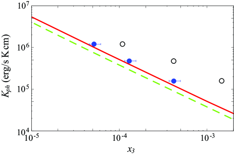
Figure 1: (Color online) Thermal conductivity of a dilute solution of ³He in superfluid ⁴He at $T$ = 0.45 K. The solid line shows the phonon thermal conductivity, in the limit in which the ³He are at rest in equilibrium, calculated with ³He recoil (see text). The dashed line shows the phonon thermal conductivity, Eq. (27), without recoil corrections. The open circles are three representative measurements at $T\sim 0.43$ K at the average $x_{3}$ reported in Ref rosenbaum ; the solid circles with the error bars are the same thermal conductivities, but shown at the corrected $x_{3}$, as discussed in Sec. VI.

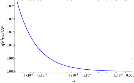
Figure 2: Ratio of the contribution of the viscous term (see Eq. (4)) to the drag on the phonons due to scattering against the ³He at a temperature of 0.45 K. The magnitude of the drag is given by the ³He pressure gradient (see Eq. (25)) as a function of ³He concentration $x_{3}$ (the concentrations measured in lamoreaux are $x_{3}=7\times 10^{-5}$ and $3\times 10^{-4}$). The viscous term is calculated for laminar flow in a circular pipe of radius $R$ = 2.5 cm, using the ⁴He viscosity measured by Greywall greywall .

We return now to justify neglecting viscous stresses in the pressure equation (4). The drag force per unit volume of the ³He on the phonons is $\sim\rho_{ph}s/\ell_{ph3}$. We assume laminar flow in a circular pipe of radius $R$, for which $\nabla^{2}\vec{v}_{ph}=-8\langle\vec{v}_{ph}\rangle/R^{2}$ is a constant throughout visc , thus overestimating the viscous force (density) on the phonons by neglecting the drag against the ³He. The phonon viscosity is $\sim\rho_{ph}s\ell_{visc}/5$, where $\ell_{visc}$ is the phonon mean free path for viscosity, and thus the ratio of the viscous force to drag force is $\sim\ell_{visc}\ell_{ph3}/R^{2}\ll 1$; see Fig. 2. In addition, the ratio of the ³He viscosity, $\sim m^{*}n_{3}\bar{v}\ell_{33}/5$ (where $\bar{v}$ is a mean ³He thermal velocity), to the phonon viscosity is of order $(n_{3}/S_{ph})(\ell_{33}/\ell_{visc})\ll 1$ here.

V Diffusion of ${}^{3}\mbox{\boldmath He}$ against phonons

We now calculate the rate of diffusion of ³He atoms in a bath of phonons at a fixed temperature $T$. In the derivation of heat transport above, we assumed that the ³He cloud was at rest and that the phonons were drifting with velocity $\vec{v}_{ph}$. In a frame in which the phonons are at rest and the ³He drift with velocity $\vec{v}_{3}$, Eq. (25) becomes

$$\nabla P_{3}=-\frac{n_{3}\Gamma}{3T}\vec{v}_{3},$$ (28)

where we use $\nabla P_{ph}=-\nabla P_{3}$. With the temperature variation in $P_{3}$ neglected, Eq. (28) becomes a familiar diffusion equation,

$$D_{3}\nabla n_{3}=-n_{3}\vec{v}_{3},$$ (29)

where

$$D_{3}=\frac{3T^{2}}{\Gamma}\sim\frac{1}{T^{7}}.$$ (30)

More generally, however, phonons drive ³He pressure gradients, rather than simply density gradients. In an arbitrary frame, the response of the ³He current to a phonon wind becomes

$$\vec{j}_{3}=n_{3}\vec{v}_{3}=n_{3}\vec{v}_{ph}-D_{3}\nabla n_{3}-D_{T}\nabla T,$$ (31)

where, in our particular case, $D_{T}=n_{3}D_{3}/T$ is an effective “thermoelectric” transport coefficient.

VI Application to experiment

To further illustrate the physics, we now determine the temperature and concentration distributions for two geometries (Refs. rosenbaum and lamoreaux ) of interest. Conservation of energy implies

$$\nabla\cdot\vec{Q}=-\nabla\cdot(K_{ph}\nabla T)=-C\nabla\left(\frac{\nabla T}{P_{3}}\right)=0,$$ (32)

where, from Eq. (27), $C=n_{4}^{2}s^{2}/90\pi J$. For simplicity, recoil effects are neglected in writing the equations here; however, they are taken into account in all numerical calculations reported below. We eliminate $P_{3}$ using the solution

$$P_{3}+\frac{1}{4}S_{ph}T=P,$$ (33)

of Eq. (6), where the constant $P$ is the total pressure of the excitations. Equation (32) then reduces to a partial differential equation in $T$ alone (even when including the recoil corrections), which we solve using the finite element code FlexPDE flexpde . Given $T(\vec{r})$, we determine $n_{3}(\vec{r})$ from Eq. (33), and determine the constant $P$ by fixing the total number of ³He atoms in the system.

We begin by applying this theoretical description to the experiment of Rosenbaum et al. rosenbaum , where the thermal conductivity of mixtures in the concentration range $1.1\times 10^{-4}\leq x_{3}\leq 1.3\times 10^{-2}$ were measured at temperatures $0.084\leq T\leq 0.65$ K. They determined the thermal conductivity by measuring the temperature difference over a 5 cm length of pipe, 0.26 cm in diameter, in the presence of a localized heat source. The pipe was connected to small reservoirs at either end containing the thermometers, the coupling to the dilution refrigerator and the heater.

In the analysis in Ref. rosenbaum , the effect of the variable ³He concentration in the pipe, and its attendant effect on the thermal conductivity, was not taken into account. We therefore determined the temperature and concentration distributions in their system by adjusting the heater power and minimum (dilution refrigerator) temperature to match the reported average temperature and the temperature difference implied by the reported thermal conductivity. We note that the ³He thermal conductivity is negligibly small owing to $\ell_{33}\ll\ell_{3ph}$, Eq. (19).

Because the phonons push the ³He into the cold reservoir, the average concentration in the pipe is substantially lower than the concentration including the reservoirs. We show the results of our calculations in Fig. 1 for representative measurements tempRange of Ref. rosenbaum . The open circles are the thermal conductivities as reported, plotted at the average overall concentration; the solid circles are plotted at the average concentrations calculated for the pipe. Because the dimensions of the reservoirs are not given in Ref. rosenbaum , there is some uncertainty in the calculated result. The error bars shown in Fig. 1 represent changes of about $\pm 25$% from the reservoir volumes estimated from the schematic in their Fig. 1. Given the uncertainties related to the geometry and the details of how the thermal conductivity was extracted, there is good agreement between this calculation and the measurement. As previously noted in Sec. III, the theoretical analysis in Ref. rosenbaum incorrectly assumed that the primary phonon relaxation was due to ³He-phonon scattering, rather than phonon-phonon scattering along rays.

We now analyze the experiment of Lamoreaux et al. lamoreaux , which measures the ³He density response to a localized heat source by a novel technique. In the experiment, a dilute solution with concentration in the range $7\times 10^{-5}$ to $3\times 10^{-4}$ is contained in a cylindrical cell roughly 5 cm in diameter and 5 cm long, cooled at one end by a dilution refrigerator to a temperature $T$ in the range $0.45-0.95$ K hayden2 . A temperature gradient is created by a resistive heater generating 7–15 mW, located roughly midway between the ends and near the cylinder wall (see Fig. 4 below). The resulting spatial distribution of the ³He density is probed by a well-collimated neutron beam of diameter $\sim$ 0.25 cm going through the cell. A fraction of the neutrons are captured via the reaction ${\rm n}+^{3}{\rm He}\rightarrow{\rm p}+{\rm t}+764\hbox{ keV}$. The XUV scintillation light from protons and tritons in the liquid ⁴He is converted to visible light and detected by a photomultiplier tube which views the solution through a window at the other end of the cell. The yield of scintillation light, measured as a function of cell temperature, initial ³He concentration, and heater power, is used to determine the thermally induced change in the ³He distribution. The heat flow again produces non-uniform temperature and ³He concentration distributions. Because the concentration and temperature gradients are directly proportional, Eq. (7), the concentration gradients implied by the measured scintillation yields here simply encode the same type of temperature difference information measured by Rosenbaum et al. We note that the proportionality constant involves $S_{ph}+n_{3}$, rather than just $S_{ph}$.

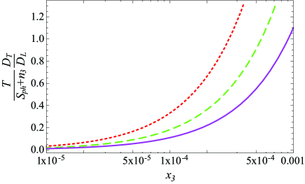
Figure 3: (Color online) Contribution of the thermoelectric transport term relative to the effective diffusion constant, $D_{L}$ extracted in Ref. lamoreaux. The temperatures are 0.45 K (dotted), 0.55 K (dashed) and 0.65 K (solid).

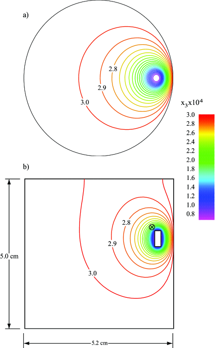
Figure 4: (Color online) An example of the ³He distribution for a cell 5.2 cm in diameter and 5.0 cm high, with refrigerator temperature 0.45 K, average $x_{3}=3\times 10^{-4}$, and heater power 15 mW. The sections are: a) perpendicular to the cylinder axis and containing the neutron beam axis; and b) perpendicular to the neutron beam (the cross in the figure) and through the center of the heat source. We assume in this simulation that the cylindrical wall of the cell is at the same temperature as that of the base where the refrigerator is attached; the top surface is insulated. The ³He concentration contours, of constant spacing, are marked in units of $10^{-4}$; the minimum is $x_{3}=0.69\times 10^{-4}$ at the surface of the heater and the maximum concentration is $3.05\times 10^{-4}$, on the lower cell boundary.

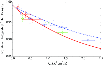
Figure 5: (Color online) Representative results of the finite element calculation, including ³He recoil, of the relative integrated ³He (column) density along the neutron beam as a function of the quantity $\xi_{L}=T^{7}\left({\cal P}/S_{ph}T\right)$ where ${\cal P}$ is the heater power, along with data from Ref. lamoreaux (circles, 0.45 K; diamonds, 0.55 K and squares, 0.65 K). The curves are for a refrigerator (and barrel) temperature of $0.45$ K: solid, $x_{3}=3\times 10^{-4}$; dotted, $x_{3}=7\times 10^{-5}$; coincidentally, the results for $T=0.65$ K and $x_{3}=3\times 10^{-4}$ are essentially the same as the dotted curve. The curves are plotted for the average temperature (greater than the boundary temperature) along the neutron beam path. For example, at the actual value $T^{6}{\cal P}/S_{ph}=2.5$, the average $\xi_{L}$ is shifted upward by $\Delta\xi_{L}\approx 0.05\,K^{7}$ cm³/s for $T$ = 0.45 K, and by $\Delta\xi_{L}\approx 0.5\,K^{7}$ cm³/s for $T=0.65$ K.

The response of the ³He density to the heat source is given here by Eq. (8). Combining this result with $\vec{Q}=TS_{ph}\vec{v}_{ph}$, one can write

$$\nabla n_{3}=\frac{S_{ph}(S_{ph}+n_{3})}{K}\vec{v}_{ph}.$$ (34)

Reference lamoreaux , which did not take into account the temperature gradient induced by the heat flow, interpreted the result for the ³He density gradient in terms of a simple diffusion constant, $D_{L}$, in the form,

$$\nabla n_{3}=\frac{n_{3}}{D_{L}}\vec{v}_{ph}.$$ (35)

From Eq. (34) we see that

$$D_{L} = \frac{n_{3}}{S_{ph}+n_{3}}\frac{K}{S_{ph}}.$$ (36)

Equivalently,

$$D_{L}=D_{3}-\frac{T}{S_{ph}+n_{3}}D_{T}=\frac{S_{ph}}{S_{ph}+n_{3}}D_{3}.$$ (37)

The $D_{T}$ term in this equation makes a significant contribution at higher concentrations (see Fig. 3); as noted, $n_{3}\sim S_{ph}$ for a large range of concentrations in the experiment of Ref. lamoreaux . This effective $D_{L}$ is not a simple diffusion constant, owing to the presence of the temperature gradient. We note that while the temperature dependence of the result for $D_{3}$ without ³He recoil falls with temperature as $1/T^{7}$, the temperature dependence of the effective $D_{L}$ differs, owing both to recoil effects and the $1/T^{3}$ dependence of $n_{3}/S_{ph}$. The relative similarity of $D_{L}$ and $D_{3}$ also depends on the ³He thermal conductivity being negligible.

An example of the ³He distribution resulting from the finite element calculation for the Lamoreaux et al. experiment is shown in Fig. 4; results of the relative integrated (column) ³He densities along the neutron beam are shown in Fig. 5 together with the data in Fig. 4 of lamoreaux . To illustrate the effect of other variables in the problem, we also show in Fig. 5 the results for $T$ = 0.65 K and for the two concentrations used in the experiment. In this calculation we take the refrigerator end and the barrel of the cell to be fixed at $T=0.45$ and $0.65$ K as indicated; the opposite end of the cell is insulated. We note that the conductivity of the aluminum barrel is more than an order of magnitude larger than that of the phonons at these temperatures AlCond . The relative column density calculated with an insulator in place of the aluminum barrel (not shown) falls well below the data. In this simulation we neglect any possibility of convective flow in the ³He. The effect of the non-zero size of the neutron beam is to reduce the calculated ratios in Fig. 5 by $\sim 0.003$ at the largest values of $\xi_{L}$, well within the reported uncertainties. The agreement of the present theory with the experiment provides further confirmation of the microscopic transport theory in the concentration range of the Lamoreaux et al. experiment.

VII Summary

We have laid out the basic transport theory of dilute solutions of ³He in superfluid ⁴He in the regime where scattering among the ³He is the primary mechanism keeping the ³He in thermal equilibrium, and phonons are the significant excitations of the ⁴He. We find that in the range of ³He concentrations in the Rosenbaum et al. rosenbaum and Lamoreaux et al. lamoreaux experiments, $7\times 10^{-5}\leq x_{3}\leq 1.5\times 10^{-3}$, heat transport is dominated by phonons. The physical response of the system is not simple diffusion, described only by a ³He diffusion constant, $D_{3}$, since the temperature gradients are important. The experiments can be characterized simply by a phonon thermal conductivity. This thermal conductivity, calculated in a microscopic framework, satisfactorily reproduces the measurements, indicating that the well-tested theory of ³He-phonon scattering in dilute solutions of ³He in superfluid ⁴He is consistent with these experiments as well.

Appendix A Recoil corrections

In this Appendix we calculate contributions to the thermal conductivity due to the finite ³He mass. We start from Eq. (24) with the structure factor (LABEL:S3withrecoil) of the ³He,

$$\nabla P_{ph}= -\vec{v}_{ph}\frac{2\pi n_{3}}{6T}\int\frac{d^{3}q}{(2\pi)^{3}}\int\frac{d^{3}q^{\prime}}{(2\pi)^{3}}n_{q}^{0}(1+n_{q^{\prime}}^{0})k^{2}|\langle{\cal T}\rangle|^{2}\left(\frac{m^{*}}{2\pi k^{2}T}\right)^{1/2}e^{-m^{*}(sq-sq^{\prime}-k^{2}/2m^{*})^{2}/2k^{2}T}.$$

$$= -\vec{v}_{ph}\frac{2\pi n_{3}}{6T}\int\frac{d^{3}q}{(2\pi)^{3}}\int\frac{d^{3}q^{\prime}}{(2\pi)^{3}}\frac{k^{2}|\langle{\cal T}\rangle|^{2}}{4\sinh(sq/2T)\sinh(sq^{\prime}/2T)}\left[\left(\frac{m^{*}}{2\pi k^{2}T}\right)^{1/2}e^{-m^{*}(sq-sq^{\prime})^{2}/2k^{2}T}\right]e^{-k^{2}/8m^{*}T}.$$

The integral in Eq. (LABEL:phBE3Appendix) is proportional to the inverse of the thermal conductivity. In the limit $m^{*}\rightarrow\infty$ the expression in square brackets reduces to $\delta(sq-sq^{\prime})$. For finite $m^{*}$ there are two effects. First, the structure factor, and therefore also the scattering rate, is reduced in magnitude because of the nonzero momentum transfer, $\vec{k}=\vec{q}-{\vec{q}}^{\prime}$, as is shown by the final Gaussian factor. Second, as the first Gaussian factor indicates, there is an energy transfer $sq-sq^{\prime}$ which is of order $(Tk^{2}/m^{*})^{1/2}\sim(T/m^{*}s^{2})^{1/2}T$.

The contributions to the scattering amplitude for nonzero energy transfer and for nonzero velocity of the ³He atoms have not been investigated in detail, although the basic processes were discussed in full in Ref. BE67 . Here we use Eq. (13) for the scattering amplitude. With prefactors omitted, the quantity to be calculated is thus

$$\int_{0}^{\infty}dq\int_{0}^{\infty}dq^{\prime}\int_{-1}^{1}d\cos\theta\frac{k(qq^{\prime})^{3}(A+B\cos\theta)^{2}}{4\sinh(sq/2T)\sinh(sq^{\prime}/2T)}e^{{-m^{*}s^{2}(q-q^{\prime})^{2}/2k^{2}T}}e^{-k^{2}/8m^{*}T}.$$ (39)

We have evaluated the integrals numerically and find, as stated in Sec. IV, that inclusion of recoil effects increases the thermal conductivity by $\sim 25-35$% in the temperature range $0.45-0.65$ K.

The leading corrections to the result for $m^{*}\rightarrow\infty$ are of relative order $T/m^{*}s^{2}$ relative to the result in the low temperature limit; we now calculate them analytically. To first order in $T/m^{*}s^{2}$ the effects of the nonzero momentum transfer and the nonzero energy transfer are additive, and we calculate each in turn. The more important term is due to the momentum transfer. When this term alone is included one finds

$${\lim_{T\rightarrow 0}(TK)}/{TK}\simeq 1-\frac{1}{8m^{*}T}\frac{\langle k^{4}\rangle}{\langle k^{2}\rangle},$$ (40)

where

$$\langle\ldots\rangle=\int_{0}^{\infty}dq\int_{-1}^{1}d\cos\theta\frac{q^{6}(A+B\cos\theta)^{2}}{4\sinh^{2}(sq/2T)}(\ldots)\,\,.$$ (41)

In these integrals we may replace $k^{2}$ by its value $2q^{2}(1-\cos\theta)$ for zero energy transfer. The integrals over $q$ and $\theta$ decouple and one finds

$$TK\simeq\left(1+\frac{T}{4m^{*}s^{2}}\frac{\tilde{J}}{J}\frac{I_{10}}{I_{8}}\right)\lim_{T\rightarrow 0}(TK),$$ (42)

where

$${\tilde{J}}=\int_{-1}^{1}\frac{d\cos\theta}{2}(A+B\cos\theta)^{2}(1-\cos\theta)^{2}$$

$$=\frac{4}{3}A^{2}-\frac{4}{3}AB+\frac{8}{15}B^{2}$$ (43)

and

$$I_{n}=\int_{0}^{\infty}dq\frac{x^{n}}{4\sinh^{2}(x/2)}=n!\,\zeta(n),$$ (44)

where $\zeta(n)$ is the Riemann zeta function of order $n$. Therefore the thermal conductivity is given by

$$K\simeq\left(1+\frac{25\pi^{2}}{11}\frac{\tilde{J}}{J}\frac{T}{m^{*}s^{2}}\right)\frac{1}{T}\lim_{T\rightarrow 0}(TK).$$ (45)

We now calculate the leading correction to the thermal conductivity due to the energy transfer, which is found by neglecting the term $k^{2}/8m^{*}T$ in the exponent in Eq. (39). The Gaussian in the energy difference has a width small compared with $T$, so we adopt a procedure similar to that used in making the Sommerfeld expansion for low temperature Fermi systems, where the derivative of the Fermi function approaches a delta function. In an integral of the form,

$$G(x)=\int_{0}^{\infty}dyg(y)\frac{e^{-(x-y)^{2}/2\Delta^{2}}}{(2\pi\Delta)^{1/2}},$$ (46)

where $\Delta$ is a constant, and the function $g(y)$ varies slowly on the scale $\Delta$, one finds on expanding $g$ in a Taylor series about $y=x$, that

$$G(x)=g(x)+\frac{\Delta^{2}}{2}g^{\prime\prime}(x)+\ldots\,\,.$$ (47)

When this result is applied to the $q^{\prime}$ integral in Eq. (39) with the final Gaussian omitted, one finds

$$\int_{0}^{\infty}dq\int_{0}^{\infty}dq^{\prime}\int_{-1}^{1}\frac{d\cos\theta}{2}\left(\frac{m^{*}s^{2}}{2\pi Tk^{2}}\right)^{1/2}\frac{k^{2}(qq^{\prime})^{3}(A+B\cos\theta)^{2}e^{-m^{*}s^{2}(q-q^{\prime})^{2}/2k^{2}T}}{4\sinh^{2}(sq/2T)}$$

$$\simeq J\int_{0}^{\infty}dq\frac{2q^{8}}{4\sinh^{2}(sq/2T)}+\frac{T}{2m^{*}s^{2}}\int_{0}^{\infty}dq\int_{-1}^{1}\frac{d\cos\theta}{2}\frac{k^{2}q^{3}k^{2}(A+B\cos\theta)^{2}}{2\sinh(sq/2T)}\left(\frac{\partial^{2}}{\partial(q^{\prime})^{2}}\frac{k^{2}q^{\prime 3}}{2\sinh(sq^{\prime}/2T)}\right)_{q^{\prime}=q},$$ (48)

which, when expressed in terms of the variables $x=sq/T,y=sq^{\prime}/T$, and $z=\cos\theta$, is proportional to

$$J\int_{0}^{\infty}dx\frac{2x^{8}}{4\sinh^{2}(x/2)}+\frac{T}{m^{*}s^{2}}\int_{0}^{\infty}dx\frac{x^{5}}{2\sinh(x/2)}\int_{-1}^{1}\frac{dz}{2}(1-z)(A+Bz)^{2}\left(\frac{\partial^{2}}{\partial y^{2}}\frac{\kappa^{2}y^{3}}{2\sinh(y/2)}\right)_{y=x},$$ (49)

where $\kappa^{2}=x^{2}+y^{2}-2xyz$. The second derivative is

$$\frac{x^{3}}{\sinh(x/2)}\left\{1+(1-z)\left[12-\frac{1}{4}x^{2}-4x\coth(x/2)+\frac{1}{2}x^{2}\coth(x/2)^{2}\right]\right\}.$$ (50)

On evaluating the integrals, one finds that the effect of energy transfer produces contributions to the integral (39) having the form

$$1+\left(1-\frac{(25\pi^{2}-198)}{33}\frac{\tilde{J}}{J}\right)\frac{T}{m^{*}s^{2}}.$$ (51)

The numerical factor $(25\pi^{2}-198)/33$ is approximately 1.477 and thus one sees that the effects of nonzero energy transfer are much less important than those due to nonzero momentum transfer. When both contributions to the thermal conductivity are included, one finds on inserting Eq. (27) for the low temperature limiting behavior,

$$K\simeq\frac{n_{4}s^{2}}{90\pi x_{3}JT}\left(1+\frac{T}{m^{*}s^{2}}\left[\frac{100\pi^{2}-198}{33}\frac{\tilde{J}}{J}-1\right]\right).$$

(52)

The coefficient of ${\tilde{J}}/J$ is approximately 23.90. For $A=-1.2$ and $B=0.70$, $J$ is 2.16, ${\tilde{J}}$ is $3.30$ and their ratio is 1.52. Thus the coefficient of $T/m^{*}s^{2}$ is 35.5. Even though $m^{*}s^{2}$ = 48.1 K, the effects of recoil are large even at temperatures well below 1 K as a consequence of the large numerical coefficient. This coefficient reflects the fact that the most important contributions to the momentum transfer arise from phonons with momenta $\gg T/s$. At $T$ = 0.5 K the correction is 37%, which is considerable. Higher-order contributions in $T$ can be significant, and one would expect these to reduce the deviation from the low-temperature limiting result by an amount of relative order $(0.37)^{2}\sim 10\%$. These analytic results are in good agreement with the numerical integration of Eq. (39) described above, and shown in Fig. 1.

References

- (1) R. Golub and S. K. Lamoreaux, Phys. Rep. 237, 1 (1994).
- (2) This experiment utilizes the absorption of ultracold polarized neutrons on polarized 3He atoms via the reaction .
- (3) R. L. Rosenbaum, J. Landau and Y. Eckstein, J. Low Temp. Phys. 16, 131 (1974).
- (4) S. K. Lamoreaux, G. Archibald, P. D. Barnes, W. T. Buttler, D. J. Clark, M. D. Cooper, M. Espy, G. L. Greene, R. Golub, M. E. Hayden, C. Lei, L. J. Marek, J.-C. Peng, and S. Penttila, Europhys. Lett. 58, 718 (2002).
- (5) M. Hayden, S. K. Lamoreaux, and R. Golub, AIP Conf. Proc. 850, 147 (2006).
- (6) G. Baym, D. H. Beck, and C. J. Pethick, to be published.
- (7) G. Baym and C. Ebner, Phys. Rev. 164, 235 (1967).
- (8) H. J. Maris, Rev. Mod. Phys. 49, 341 (1977).
- (9) G. Baym, R. G. Barrera, and C. J. Pethick, Phys. Rev. Lett. 22, 20 (1969).
- (10) R. M. Bowley, Europhys. Lett. 58, 725 (2002).
- (11) The phonon contributions to the dissipative second viscosity terms in the superfluid acceleration equation vanish, see khalat1 .
- (12) I. M. Khalatnikov, Introduction to the Theory of Superfluidity, (W. A. Benjamin, New York, 1965), pp. 65,133.
- (13) I. M. Khalatnikov, op. cit., ch. 25; I. M. Khalatnikov and V. N. Zharkov, Zh.E.T.F. 32, 1108 (1957) [Engl. transl. Sov. Phys. JETP 5, 905 (1957)].
- (14) J. Wilks, The Properties of Liquid and Solid Helium, (Clarendon Press, Oxford, 1967), sec. 9.5.
- (15) L. D. Landau and E. M. Lifshitz, Fluid Mechanics (Pergamon Press, 1987), Sec. 59.
- (16) G. Baym and C. Ebner, Phys. Rev. 170, 346 (1968).
- (17) Note that in the implementation of this correction in Ref. Bowley , the 3He effective mass is taken to be one third of its actual value, and therefore the effects of recoil are overestimated.
- (18) One should not be alarmed by the apparent divergence as . When becomes sufficiently small, the 3He no longer provide the mechanism for absorbing momentum from the phonons, and rather the phonon thermal conductivity becomes limited by viscous transfer of momentum from the phonons to the container walls BBPII .
- (19) C. Boghosian and H. Meyer, Phys. Lett. A25, 352 (1967).
- (20) G. E. Watson, J. D. Reppy, and R. C. Richardson, Phys. Rev. 188, 384 (1969).
- (21) B. M. Abraham, C. G. Brandt, Y. Eckstein, J. Munarin, and G. Baym, Phys. Rev. 188, 309 (1969).
- (22) In fact, the viscosity for flow in a circular pipe plays a role only in a thin boundary layer, which for the concentrations and temperatures under consideration is of order mm thick.
- (23) D. S. Greywall, Phys. Rev. B 23, 2152 (1981).
- (24) PDE Solutions Inc., Spokane Valley, WA 99206 USA.
- (25) We note that the analysis here must be extended for the lower temperatures in the experiment to include scattering from the walls. For example, the phonon mean free path is larger than the diameter of the pipe for temperatures below about 0.37 K.
- (26) We are grateful to M. Hayden, private communication, for the details of the geometry.
- (27) C. B. Satterthwaite, Phys. Rev. 125, 873 (1962), R. M. Mueller, C. Buchal, T. Oversluizen, and F. Pobell, Rev. Sci. Instrum. 49, 515 (1978) and references therein.