Large-scale Ferrofluid Simulations on Graphics Processing Units

Abstract

We present an approach to molecular-dynamics simulations of ferrofluids on graphics processing units (GPUs). Our numerical scheme is based on a GPU-oriented modification of the Barnes-Hut (BH) algorithm designed to increase the parallelism of computations. For an ensemble consisting of one million of ferromagnetic particles, the performance of the proposed algorithm on a Tesla M2050 GPU demonstrated a computational-time speed-up of four order of magnitude compared to the performance of the sequential All-Pairs (AP) algorithm on a single-core CPU, and two order of magnitude compared to the performance of the optimized AP algorithm on the GPU. The accuracy of the scheme is corroborated by comparing the results of numerical simulations with theoretical predictions.

1 Introduction

Ferrofluids are media composed of magnetic nanoparticles of diameters in the range $10\div 50$ nm which are dispersed in a viscous fluid (for example, water or ethylene glycol) [1]. These physical systems combine the basic properties of liquids, i.e. a viscosity and the presence of surface tension, and those of ferromagnetic solids possessing, i.e. an internal magnetization and high permeability to magnetic fields. This synergetic duality makes ferrofluids an attractive candidate for performing different tasks, ranging from the delivery of rocket fuel into spacecraft’s thrust chambers under zero-gravity conditions to the high-precision drug delivery during cancer therapy [2]. Moreover, ferrofluids have already found their way into commercial applications as EM-controlled shock absorbers, dynamic seals in engines and computer hard-drives, and as key elements of high-quality loudspeakers, to name but a few [3].

Being liquids, ferrofluids can be modeled by using different macroscopic, continuum-media approaches. The corresponding field, ferrohydrodynamics [1], is a well-established area that has produced a lot of fundamental results. However, some important phenomena such as magnetoviscosity [4, 5] cannot be described properly neither on the hydrodynamical level nor within the single-particle picture [6]. The role of multiparticle aggregates – chains and clusters – living in the ferrofluid bulk, is important there. The evaluation of other non-Newtonian features of ferrofluids, which can be controlled by external magnetic fields [5], also demands information about structure of aggregates and their dynamics. The key mechanism responsible for the formation of ferro-clusters is the dipole-dipole interaction acting between magnetic particles. Under certain conditions, the interaction effects can overcome the destructive effects of thermal fluctuations and contribute tangibly to the ensemble dynamics. Therefore, in order to get a deeper insight into the above-mentioned features of ferrofluids, the interaction effects should be explicitly included into the model.

Strictly speaking, the dipole-dipole interaction acts between all the possible pairs of $N$ ferromagnetic particles. Therefore, the computational time of the straightforward sequential algorithm scales like $N^{2}$. This is a fundamental drawback of many-body simulations and standard, CPU-based computational resources often limit the scales of the molecular-dynamics calculations. In order to run larger ensembles for longer times, researchers either (i) advance their models and numerical schemes and/or (ii) rely on more efficient computers. The first track led to different methods developed to explore the equilibrium properties of bulk ferrofluids. Most prominent are cut-off sphere approximations [7] and the Ewald summation technique [8], see also Ref. [9] for different modifications of the technique. However, both methods are of limited use for computational studies of confined ferrofluids, a problem that attracts special attention nowadays due to its practical relevance [10, 11]. An alternative approach is the search for ways to increase scalability and parallelism of computations, see Ref. [12]. Until recently, this practically meant the use of either large computational clusters, consisting of many Central Processing Units (CPUs), or massively parallel supercomputers, like Blue Gene supercomputers. The prices and the maintenance costs of such devices are high. The advent of the general-purpose computing on graphics processing units (GP²U) [13] has changed the situation drastically and boosted simulations of many-body systems onto new level [14]. GPUs, initially designed to serve as the data pipelines for graphical information, are relatively small, much easier to maintain, and possess high computation capabilities allowing for parallel data processing. Nowadays, the scientific GPU-computing is used in many areas of computational physics, thanks to the Compute Unified Device Architecture (CUDA) developed by NVIDIA Corporation [15]. CUDA significantly simplifies GPU-based calculations so now one could use a Sony PlayStation 3 as a multi-core computer by programming it with $C$, $C++$ or $Fortran$ [16] languages.

The typical scale of molecular-dynamics simulations in ferrofluid studies is within the range $N=10^{2}-10^{3}$ [17, 18], while $N=10^{4}$ constitutes the current limit [19]. It is evident that the increase of the ensemble size by several orders of magnitude would tangibly improve the statistical sampling and thus the quality of simulation results. To run numerically $10^{5}\div 10^{6}$ interacting magnetic particles is a task not much different from the running of an artificial Universe [20]. Therefore, similar to the case of Computational Cosmology [21, 22, 23], the GP²U seems to be very promising also in the context of ferrofluid simulations. In this paper we report the performance of a recently proposed GPU-oriented modification of the Barnes-Hut algorithm [24] used to simulate the dynamics of $N=10^{3}\div 10^{6}$ interacting ferromagnetic particles moving in a viscous medium.

Although being mentioned as a potentially promising approach (see, for example, Ref. [25]), the Barnes-Hut algorithm was never used in molecular-dynamics ferrofluid simulations, to the best of our knowledge. Our main goal here is to demonstrate a sizable speed-up one can reach when modeling such systems on a GPU – and by using GPU-oriented numerical algorithms – compared to the performance of conventional, CPU-based algorithms. We also demonstrate the high accuracy of the Barnes-Hut approximation by using several benchmarks. The paper is organized as follows: First, in Section II we specify the model. Then, in Section III, we describe how both, the All-Pairs and Barn-Hut algorithms, can be efficiently implemented for GPU-based simulations. The results of numerical tests are presented and discussed in Section V. Finally, Section VI contains conclusions.

2 The model

The model system represents an ensemble of $N$ identical particles of the radius $R$, made of a ferromagnetic material of density $D$ and specific magnetization $\mu$. Each particle occupies volume $V=\frac{3}{4}\pi R^{3}$, has magnetic moment $\vec{m}=\vec{m}(t)$ of constant magnitude $|\vec{m}|=m=V\mu$, mass $M=VD$, and moment of inertia $I=\frac{2}{5}MR^{2}$. The ensemble is dispersed in a liquid of viscosity $\eta$. Based on the Langevin dynamics approach, the equations of motions for $k$-th nanoparticle can be written in the following form [17]

$$I\ddot{\theta_{k}}\! = \!N_{kz}-G_{r}\dot{\theta}_{k}+\Xi^{r}_{\theta},$$ (1)

$$I\ddot{\varphi_{k}}\! = \!-N_{kx}\sin\varphi_{k}+N_{ky}\cos\varphi_{k}-G_{r}\dot{\varphi}_{k}+\Xi^{r}_{\varphi},$$ (2)

$$M\ddot{\vec{r}}_{k}\! = \!\mu_{0}(\vec{m}_{k}\nabla_{k})\cdot\vec{H}_{k}+\vec{F}_{k}^{sr}-G_{d}\dot{\vec{r}}_{k}+\vec{\Xi}^{d}_{\vec{r}},$$ (3)

where $\theta$ and $\varphi$ are the polar and azimuthal angles of the magnetization vector $\vec{m}$ respectively. $N_{kx}=m_{ky}H_{kz}-m_{kz}H_{ky},N_{ky}=m_{kz}H_{kx}-m_{kx}H_{kz},N_{kz}=m_{ky}H_{kx}-m_{kx}H_{ky}$, $x,y,z$ denotes the Cartesian coordinates, dots over the variables denote the derivatives with respect to time. $\vec{r}_{k}$ is the radius-vector defining the nanoparticle position, and the gradient is given by $\nabla_{k}=\frac{\partial}{\partial\vec{r}_{k}}=\vec{e}_{x}\frac{\partial}{\partial x_{k}}+\vec{e}_{y}\frac{\partial}{\partial y_{k}}+\vec{e}_{z}\frac{\partial}{\partial z_{k}}$, ($\vec{e}_{x},\vec{e}_{y},\vec{e}_{z}$ are the unit vectors of the Cartesian coordinates). Constants $G_{t}=6\pi\eta R$, and $G_{r}=8\pi\eta R^{3}$ specify translational and rotational friction coefficients, $\mu_{0}=4\pi\cdot 10^{-7}\mathrm{H}/\mathrm{m}$ is the magnetic constant.

The resulting field acting on the $k$-th particle $\vec{H}_{k}$ is the sum of external field $\vec{H}^{ext}$ and overall field exerted on the particle by the rest of the ensemble,

$$\vec{H}_{k}\! = \!\sum_{j=1,j\neq k}^{N}{\vec{H}_{kj}^{dip}}+\vec{H}^{ext},$$ (4)

$$\vec{H}_{kj}^{dip}\! = \!\frac{3\vec{r}_{kj}(\vec{m}_{j}\vec{r}_{kj})-\vec{m}_{j}{\vec{r}_{kj}}^{\,2}}{|\vec{r}_{kj}|^{5}},$$ (5)

where $\vec{r}_{kj}=\vec{r}_{k}-\vec{r}_{j}$. $\vec{F}_{k}^{sr}$ in Eq. 3 denotes the force induced by a short-range interaction potential. In this paper we use Lennard-Jones potential [17] (though hard sphere [26], soft sphere [27] and Yukawa-type [28] potentials can be used as alternatives), so that

$$\vec{F}_{k}^{sr}=24E\sum_{j=1,j\neq k}^{N}{\frac{\vec{r}_{kj}}{\vec{r}_{kj}^{\,2}}\left[{{\left(\frac{s}{\vec{r}_{kj}}\right)}^{12}-\left(\frac{s}{\vec{r}_{kj}}\right)^{6}}\right]}.$$ (6)

Here $E$ is the depth of the potential well and $s$ is the equilibrium distance at which the inter-particle force vanishes. The interaction between a particle and container walls is also modeled with a Lennard-Jones potential of the same type. The random-force vector, representing the interaction of a particle with thermal bath, has standard white-noise components, $\langle\Xi_{\alpha}^{r}(t)\rangle=0$ ($\alpha=\varphi,\theta$), $\langle\Xi_{\beta}^{d}(t)\rangle=0$ ($\beta=x,y,z)$, and second moments satisfying $\langle\Xi_{r\alpha}(t)\Xi_{r\beta}(t^{\prime})\rangle=3k_{\rm B}TG_{r}\delta_{\alpha\beta}\delta(t-t^{\prime})\ (\alpha,\beta=\varphi,\theta)$ $\langle\Xi_{d\alpha}(t)\Xi_{d\beta}(t^{\prime})\rangle=2k_{\rm B}TG_{t}\delta_{\alpha\beta}\delta(t-t^{\prime})\ (\alpha,\beta=x,y,z)$ [17]. Here $k_{\rm B}$ is the Boltzmann constant and $T$ is the temperature of the heat bath.

By rescaling the variables, $\tau=t/T_{ch},(T_{ch}=R/\mu\sqrt{3D/4\mu_{0}}),\vec{u}=\vec{m}/|\vec{m}|,\vec{\rho}_{k}=\vec{r}_{k}/R$, ${\nabla_{\rho_{k}}}=\frac{1}{R}\frac{d}{d\vec{\rho}_{k}}$, the equations of motions for the $k-$th particle can be rewritten in the reduced form,

$$\frac{2}{5}\cdot\frac{d^{2}\theta_{k}}{d\tau^{2}}\! = \!(u_{kx}h_{ky}-u_{ky}h_{kx})-\varGamma_{r}\frac{d\theta_{k}}{d\tau}+\frac{T_{ch}^{2}}{VR^{2}D}\xi^{r}_{\theta}\$$ (7)

$$\frac{2}{5}\cdot\frac{d^{2}\varphi_{k}}{d\tau^{2}}\! = \!-(u_{ky}h_{kz}-u_{kz}h_{ky})\sin\varphi_{k}+(u_{kz}h_{kx}-u_{kx}h_{kz})\cos\varphi_{k}-\varGamma_{r}\frac{d\varphi_{k}}{d\tau}+\frac{T_{ch}^{2}}{VR^{2}D}{\xi^{r}_{\varphi}}\$$ (8)

$$\frac{d^{2}\vec{\rho}_{k}}{d\tau^{2}}\! = \!\vec{f}_{k}^{dip}+\vec{f}_{k}^{sr}-\varGamma_{d}\frac{d\vec{\rho}_{k}}{d\tau}+\frac{T_{ch}^{2}}{VRD}{\vec{\xi}_{\vec{\rho}}^{d}}$$ (9)

where

$$\vec{h}_{k}\! = \!\sum_{j=1,j\neq k}^{N}{\vec{h}_{kj}^{dip}}+\vec{h}^{ext},$$ (10)

$$\vec{h}_{kj}^{dip}\! = \!\frac{3\vec{\rho}_{kj}(\vec{u}_{j}\vec{\rho}_{kj})-\vec{u}_{j}\vec{\rho}_{kj}^{\,2}}{\rho_{kj}^{\,5}},$$ (11)

$$\vec{f}_{k}^{dip}\! = \!\sum_{j=1,j\neq k}^{N}\left[3\frac{\vec{\rho}_{kj}(\vec{u}_{j}\vec{u}_{k})+\vec{u}_{k}(\vec{u}_{j}\vec{\rho}_{kj})+\vec{u}_{j}(\vec{u}_{k}\vec{\rho}_{kj})}{\rho_{kj}^{\,5}}-15\frac{\vec{\rho}_{kj}(\vec{u}_{k}\vec{\rho}_{kj})(\vec{u}_{j}\vec{\rho}_{kj})}{\rho_{kj}^{\,7}}\right],$$ (12)

$$\vec{f}_{k}^{sr}\! = \!24\varepsilon\sum_{j=1,j\neq k}^{N}\frac{\vec{\rho}_{kj}}{\vec{\rho}_{kj}^{\,2}}\left[{\left(\frac{\sigma}{\rho_{kj}}\right)}^{12}-{\left(\frac{\sigma}{\rho_{kj}}\right)}^{6}\right],$$ (13)

Here $\vec{h}^{ext}=3\vec{H}^{ext}/4\pi\mu,\varGamma_{t}=G_{t}T_{ch}/VD,\varGamma_{r}=G_{r}T_{ch}/VR^{2}D,\sigma=s/R,\varepsilon=E{T_{ch}}^{2}/VRD,\vec{\rho}_{kj}=\vec{\rho}_{k}-\vec{\rho}_{j}$

Random-force vector components are given now by white Gaussian noises, with the second moments satisfying $\langle{\xi_{\alpha}^{r}}(\tau){\xi_{\beta}^{r}}(\tau^{\prime})\rangle=3k_{\rm B}T\varGamma_{r}\delta_{\alpha\beta}\delta(\tau-\tau^{\prime})/T_{ch}$ $(\alpha,\beta=\varphi,\theta)$ $\langle\xi_{\alpha}^{d}(\tau)\xi_{\beta}^{d}(\tau^{\prime})\rangle=2k_{\rm B}T\varGamma_{t}\delta_{\alpha\beta}\delta(\tau-\tau^{\prime})/T_{ch}$ $(\alpha,\beta=x,y,z)$. In general case the characteristic relaxation time of particle magnetic moments to their equilibrium orientations is much smaller than $T_{ch}$, and one can neglect the magnetization dynamics by assuming that the direction of the vector $\vec{m}_{k}$ coincides with the easy axis of the $k-$th particle. We assume that this condition holds for our model.

3 Two approaches to many-body simulations on GPUs: the All-Pairs and the Barnes-Hut algorithms

In this section we discuss two alternative approaches to the numerical propagation of the dynamical system given by Eqs. (7 - 9) on a GPU. It is assumed that the reader is familiar with the basics of the GP²U, otherwise we address him to Refs. ([29, 30]) that contain crash-course-like introductions into the physically-oriented GPU computing.

3.1 All-Pair Algorithm

The most straightforward approach to propagate a system of $N$ interacting particles is to account for the interactions between all pairs. Although exact, the corresponding All-Pairs (AP) algorithm is slow when performed on a CPU, so it is usually used to propagate systems of $N=10^{2}\div 10^{3}$ particles. However, even with this brute-force method one can tangibly benefit from GPU computations by noticing that the AP idea fits CUDA architecture [31].

One integration step of the standard AP algorithm is performed in two stages. They are:

1. Calculation of increment of particle positions and magnetic moments directions.

2. Update particle positions and magnetic moments directions.

This structure remains intact in the GPU version of the algorithm. Kernels responsible for the first stage compute forces that act on the particles, and calculate the corresponding increments for particle positions and magnetic moments, according to equations (7 - 9). The increments are then written into the global memory. Finally, second-stage kernels update particle states with the obtained increments. There is, however, a need for the global synchronization of the threads that belong to the different blocks after every stage since the stages are performed on separate CUDA kernels and all the information about the state of the system is kept in the shared memory.

Each thread is responsible for one particle of the ensemble, and thus it should account for the forces exerted on the particle by the rest of the ensemble. To speed up the computational process we keep the data vector of the thread particle in the shared memory, as well as the information on other particles, needed to compute the corresponding interaction forces. Thus we have two sets of arrays of data in the shared memory, namely

1. data of the particles assigned to the threads of the block;

2. data of particles to compute interaction with.

The necessary data are the coordinates of the particles and projections of their magnetic moment vectors onto $x$, $y$ and $z$ axis. Size of the arrays are equal to the number of threads per block. The first set of the data is constant during one integration step, but the second set is changed. So, at the beginning we upload the information on particle coordinates and momenta to the second set of arrays in the shared memory. After computing the forces acting on the block particles, the procedure is repeated, i. e. the information on another set of particles is written into the second set of arrays and the corresponding interactions are computed. The corresponding pseudo-code is presented the below.

Algorithm 1 A CUDA kernel that computes increments.

1:cached $k\leftarrow blockIdx.x\cdot blockDim.x+threadIdx.x$

2:for $j=0$ to $numberOfParticles$ do

3:     upload to the shared memory particle positions and angles

4:     e.g. $x_{shared}[threadIdx.x]=x_{global}[ind]$, etc.

5:     for $i=0$ to $blockDim.x$ do

6:         if $j+i\neq k$  then $\triangleright$ the condition to avoid particle on-self influence

7:              Calculate force and dipole field for the particle number $j+i$

8:              on current $k$-th particle, and add the result to

9:              the total cached $\vec{f}^{dip}$, $\vec{f}^{sr}$, $\vec{h}^{dip}$.

10:         end if

11:     end for

12:     __syncthreads();

13:     $j\leftarrow j+blockDim.x$

14:end for

15:Update cached $\varDelta\rho_{x}$, $\varDelta\rho_{y}$, $\varDelta\rho_{z}$, $\varDelta\theta$, $\varDelta\varphi$ according to equations 7 - 9.

16:Copy increments to global memory.

The advantage of the described approach is that it uses the global memory in the most optimal way. The access to global memory is coalesced and there are no shared memory bank conflicts. For an ensemble $N=10^{4}$ particles this leads to the GPU occupancy of 97.7%.

3.2 Barnes-Hut Algorithm

The All-Pairs algorithm is simple and straightforward for implementation on a GPU and perfectly fits CUDA. Yet this algorithm is purely scalable. The corresponding computation time grows like $O(N^{2})$, and its performance is very slow already for an ensemble of $10^{5}$ particles.

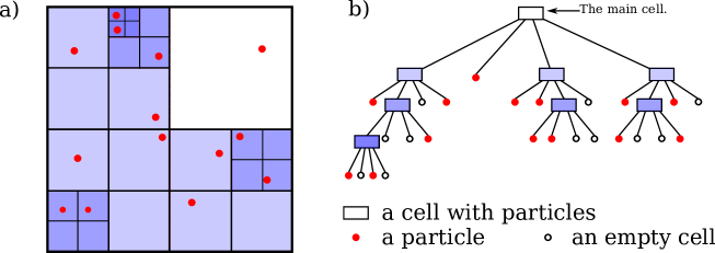
Figure 1: Barnes-Hut hierarchical decomposition in two-dimensional space and the corresponding octree. See Section 3.2 for more details.

The Barnes-Hut (BH) approximation [32] exhibits a much better scalability and its computational time grows like $O(N\log N)$. The key idea of the algorithm is to substitute a group of particles with a single pseudo-particle mimicking the action of the group. Then the force exerted by the group on the considered particle can be replaced with the force exerted by the pseudo-particle. In order to illustrate the idea assume that all particles are located in a three-dimensional cube, which is named ’main cell’. The main cell is divided then into eight sub-cells. Each sub-cell confines subset of particles. If there are more than one particle in the given sub-cell then the last is again divided into eight sub-cells. The procedure is re-iterated until there is only one particle or none left in each sub-cell. In this way we can obtain an octree with leaves that are either empty or contain single particle only. A simplified, two-dimensional realization of this algorithm is sketched with Fig. 1. By following this recipe, we can assign to every cell, obtained during the decomposition, a pseudo-particle, with magnetic moment $\vec{u^{\prime}}$ equals to the sum of magnetization vectors $\vec{u}$ of all particles belonging to the cell, and position $\vec{\rho^{\prime}}$ which is the position of the set geometric center,

$$\vec{\rho^{\prime}}=\frac{\sum\limits_{i=1}^{N^{\prime}}{\vec{\rho}_{i}}}{N^{\prime}},$$ (14)

where $N^{\prime}$ is a number of particles in the cell and $\vec{\rho}_{i}$ is the position of the $i$-th particle from the sub-set.

Forces acting on $k$-th particle can be calculated by traversing the octree. If the distance from the particle to the pseudo-particle that corresponds to the root cell is large enough, the influence of this pseudo-particle on the $k$-th particle is calculated; otherwise pseudo-particles of the next sub-cells are checked etc (sometime this procedure can lead finally to a leaf with only one particle in the cell left). Thus calculated force is added then to the total force acting on the $k$-th particle.

The BH algorithm allows for a high parallelism and it is widely employed in computational astrophysics problems [33]. However, implementation of the Barnes-Hut algorithm on GPUs remained a challenge until recently, because the procedure uses an irregular tree structure that does not fit the CUDA architecture well. It is the main reason why the BH scheme was not realized entirely on a GPU but some part of calculations was always delegated and performed on a CPU [34, 35]. A realization of the algorithm solely on a GPU has been proposed in 2011 [24]. Below we briefly outline the main idea and specify its difference from the standard, CPU-based realization.

To build an octree on a CPU usually heap objects are used. These objects contain both child-pointer and data fields, and their children are dynamically allocated. To avoid time-consuming dynamic allocation and accesses to heap objects, an array-based data structure should be used. Since we have several arrays responsible for variables, the coalesced global memory access is possible. Particles and cells can have the same data fields, e.g. positions. In this case the same arrays are used.

In contrast to the All-Pairs algorithm, where only two kernels were involved, in the original GPU-BH algorithm has six kernels [24]:

1. Bounding box definition kernel.

2. Octree building kernel.

3. Computing geometrical center and total magnetic moment of each cell.

4. Sorting of the particles with respect to their positions.

5. Computing forces and fields acting on each particle.

6. Integration kernel.

Kernel 1 defines the boundaries of the root cell. Though the ensemble is confined to a container and particles cannot go outside, we keep this kernel. The size of the root cells can be significantly smaller than the characteristic size of the container. Moreover, the computation time of this kernel is very small, typically much less than 1% of the total time of one integration step. The idea of this kernel is to find minimum and maximum values of particle positions. Here we use atomic operations and built-in $min$ and $max$ functions.

Kernel 2 performs hierarchical decomposition of the root cell and builds an octree in the three-dimensional case. As well as in following kernels, the particles are assigned to the threads in round-robin fashion. When a particle is assigned to a thread, it tries to lock the appropriate child pointer. In the case of success, the thread rewrites the child pointer and releases a lock. To perform a lightweight lock, that is used to avoid several threads access to the same part of the tree array, atomic operation should be involved. To synchronize the tree-building process we use the ${\_\_syncthreads}$ barrier.

Kernel 3 calculates magnetic moments and positions of pseudo-particles associated with cells by traversing un-balanced octree from the bottom up. A thread checks if magnetic moment and geometric center of all the sub-cells assigned to its cell have already been computed. If not then the thread updates the contribution of the ready cells and waits for the rest of the sub-cells. Otherwise the impact of all sub-cells is computed.

Kernel 4 sorts particles in accordance to their locations. This step can speed up the performance of the next kernel due to the optimal global memory access.

Kernel 5 first calculates forces acting on the particles, and then calculates the corresponding increments. Then,in order to compute the force and dipole field acting upon the particle, the octree is traversed. To minimize thread divergence, it is very important that spatially close particles belong to the same warp. In this case the threads within the warp would traverse approximately the same tree branches. This has already been provided by kernel 4. The necessary data to compute interaction are fetched to the shared memory by the first thread of a warp. This allows to reduce number of memory accesses.

Finally, kernel 6 updates the state of the particles by using the position increments and re-orient particle magnetic moments.

The above-described algorithm has many advantages. Among them are minimal thread divergence and the complete absence of GPU/CPU data transfer (aside of the transfer of the final results), optimal use of global memory with minimal number of accesses, data field re-use, minimal number of locks etc. All this allows to achieve a tangible speed-up. For more detailed description we direct the interested reader to Ref. [24].

4 Results

We performed simulations on (i) a PC with Intel Xeon x5670 @2.93GHz CPU(48 Gb RAM) and (ii) a Tesla M2050 GPU. Though the CPU has six cores, only a single core was used in simulations. The programs were compiled with nvcc (version 4.0) and gcc (version 4.4.1) compilers. Since there was no need in high-precision calculations, we used single-precision variables (float) and compiled the program with -use_fast_math key. We also used -O3 optimization flag to speedup our programs. Finally, the Euler-Maruyama method with time step $\Delta\tau=0.001$ was used to integrate Eqs. (7 - 9).

We measured the computation time of one integration step for both algorithms as functions of $N$. The results are presented with Table 1. The benefits of the GPU computing increase with the number of particles. For an ensemble of $N=10^{6}$ particles the speed-up gained from the use of the Barnes-Hut algorithm is almost $300$ compared to the performance of the performance of the optimized All-Pairs algorithm on the same GPU. However, for $N=10^{3}$ the All-Pairs algorithm performs better. It is because the computational expenses for the tree-building phase, sorting etc., overweight the speed-up effect of the approximation for small number of particles. Here we remind that $N=10^{3}$ was the typical scale of the most of ferrofluid simulations to date [17, 18].

$N$	$AP_{CPU}$	$BH_{CPU}$	$AP_{GPU}$	$BH_{GPU}$	$\frac{AP_{CPU}}{AP_{GPU}}$	$\frac{AP_{CPU}}{BH_{GPU}}$	$\frac{AP_{GPU}}{BH_{GPU}}$
$10^{3}$	34	9.8	0.7	2	49	17	0.35
$10^{4}$	3 470	137	20	6.5	174	534	3.1
$10^{5}$	392 000	2 487	1 830	54	214	7 259	33.9
$10^{6}$	39 281 250	73 121	184 330	621	213	63 214	297

Table 1: Duration of single integration step (ms) for the optimized All-Pairs algorithm implemented on CPU ($AP_{CPU}$) and GPU ($AP_{GPU}$), and for the CPU- ($BH_{CPU}$) and GPU-oriented ($BH_{GPU}$) Barnes-Hut algorithm.

Fig. 2 shows instantaneous configurations obtained during the simulations for a cubic confinement and for a mono-layer. To simulate a mono-layer of particles we use a rectangular parallelepiped of the height $2.1R$ as a confinement. The parameters of the simulations correspond to the regime when the average dipole energy is much larger than the energy of thermal fluctuations. The formation of chain-like large-scale clusters [36] is clearly visible.

5 A benchmark test: average magnetization curves

In order to check the accuracy of the numerical schemes we calculated the reduced magnetization curve [36]. Reduced magnetization vector is given by the sum $\langle\vec{u}\rangle=1/N\sum\limits_{i=1}^{N}{\vec{u}_{i}}$. The main parameters that characterize ferrofluid magnetic properties are the dipole coupling constant $\lambda$, which is the ratio of dipole-dipole potential and thermal energy, namely [37],

$$\lambda=\frac{\mu_{0}m^{2}}{16\pi R^{3}k_{\rm B}T},$$ (15)

and the volume fraction, which is the ratio between the volume occupied by particles and the total volume occupied by the ferrofluid, $V_{f}$, i.e.,

$$\phi=\frac{4/3\pi R^{3}N}{V_{f}}\cdot 100\%.$$ (16)

In the limit when $\lambda<1$ and for small volume fraction, $\phi\ll 100\%$, the projection of the reduced magnetization vector on the direction of applied field, $\langle u_{\vec{H}}\rangle$, can well be approximated by the Langevin function [36]:

$$\langle u_{\vec{H}}\rangle=L(\alpha)=\coth(\alpha)-\frac{1}{\alpha},$$ (17)

where $\alpha$ denotes the ratio between magnetic energy and thermal energy,

$$\alpha=m\mu_{0}H/k_{\rm B}T.$$ (18)

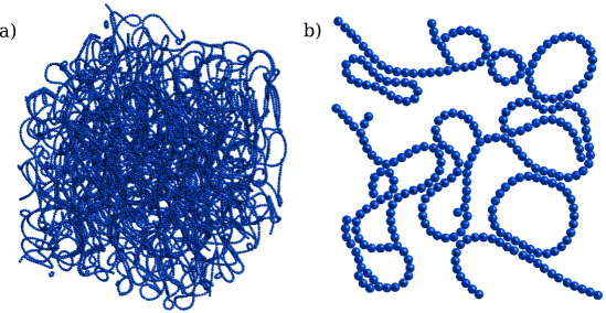
Figure 2: Snapshots of $N$-particle ensembles obtained with the Barnes-Hut algorithm: (a) $N=20\>000$ (cubic confinement with the edge length $L=150R$) and (b) mono-layer of $N=300$ particles. The parameters are: $\varGamma_{r}=\varGamma_{d}=0.1$, $T=300$ K, $\mu=3.1\cdot 10^{5}$ A/m, $D=5000$ $\rm{kg/m^{3}}$, $R=10$ nm.

We simulated a system with the parameters corresponding to maghemite ($\gamma-\rm{Fe_{2}O_{3}}$) with a saturation magnetization of $\mu=3.1\cdot 10^{5}$ A/m and density $D=5000$ $\rm{kg/m^{3}}$, the carrier viscosity $\eta=0.89\cdot 10^{-3}$ Pa (the latter corresponds to the water viscosity at $T=298$ K). The volume fraction is set at $\phi=1\%$ and the particle radius $R=3$ nm. The external magnetic field $\vec{H}$ was applied along $z-$axis. We initiated the system at time $\tau=0$ by randomly distributing particles in a cubic container. The orientation angles of particle magnetization vectors were obtained by drawing random values from the interval $[0,2\pi]$.

Fig. 3 presents the results of the simulations. After the transient $\tau_{eq}=1000$, given to the system of $N=10^{5}$ particles to equilibrate, the mean reduced magnetization has been calculated by averaging $\langle u_{z}\rangle$ over the time interval $\tau_{calc}=1000$. It is noteworthy that even single-run results are very close to the Langevin function, see Fig. 3(a). The contribution of the magnetostatic energy grows with $\alpha$ so that the strength of the dipole-dipole interaction is also increasing, see Fig. 4.

Since the average value of dipole field projection on $z$ axis is positive and increases with $\alpha$, the dipole field amplifies the external magnetic field. This explains the discrepancy between the analytical and numerical results obtained for large values of $\alpha$. For an ensemble of $N=10^{3}$ particles the results obtained with two algorithms are near identical, Fig. 3 (b).

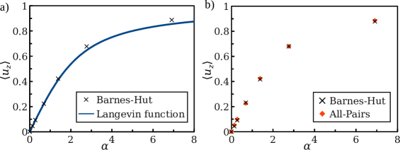
Figure 3: Checking the Barnes-Hut approximation: a) comparison between the single-run results obtained with $N=10^{5}$ particles and Langevin function, Eq. (17); b) comparison of the results obtained with the All-Pair and the Barnes-Hut algorithms for an ensemble of $N=10^{3}$ particles.

It is important also to compare the average dipole fields, $\langle h^{dip}\rangle$, calculated with the Barnes-Hut and the All-Pairs algorithms. The outputs obtained for the above-given set of parameters are shown on Fig.4. Again, two algorithms produced almost identical results.

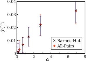
Figure 4: $z$-component of the reduced average dipole field as a function of $\alpha$ [18]. The parameters are the same as in Fig. 3(b). Each point was obtained by averaging over $10^{3}$ independent realizations.

6 Conclusions

With this work we demonstrate that the Barnes-Hut algorithm can be efficiently implemented for large-scale, GPU-based ferrofluid simulations. Overall, we achieved a speed-up more than two orders of magnitude when compared to the performance of a common GPU-oriented All-Pairs algorithm. The proposed approach allows to increase the size of ensembles by two orders of magnitude compared to the present-day scale of simulations [19]. The Barnes-Hut algorithm correctly accounts for the dipole-dipole interaction within an ensemble of $N=10^{6}$ particles and produces results that fit the theoretical predictions with high accuracy. Our finding opens several interesting perspectives. First, it brings about possibilities to perform large-scale molecular-dynamics simulations for the time evolution of ferrofluids placed in confinements of complex shapes like thin vessels or tangled pipes, where the boundary effects play an important role [38]. It is also possible to explore the non-equilibrium dynamics of ferrofluids, for example, their response to different types of externally applied magnetic fields, such as periodically alternating fields [39], or gradient fields [40]. Another direction for further studies is the exploration of the relationship between shape and topology of nano-clusters and different macroscopic properties of ferrofluids [41, 42]. Finally, the GPU-based computational algorithms provide with new possibilities to study heat transport processes in ferrofluids [43], for example to investigate the performance of ferromagnetic particles as heat sources for magnetic fluid hyperthermia [44].

7 Acknowledgment

A.Yu.P. and T.V.L. acknowledge the support of the Cabinet of Ministers of Ukraine obtained within the Program of Studying and Training for Students, PhD Students and Professor’s Stuff Abroad and the support of the Ministry of Education, Science, Youth, and Sport of Ukraine (Project No 0112U001383). S.D. and P.H. acknowledge the support by the cluster of excellence Nanosystems Initiative Munich (NIM).

References

- Rosensweig [1985] R. Rosensweig, Ferrohydrodynamics, Cambridge University Press, 1985.
- Pankhurst et al. [2003] Q. Pankhurst, J. Connolly, S. Jones, J. Dobson, Applications of magnetic nanoparticles in biomedicine, J. Phys. D Appl. Phys. 36 (2003) R167.
- Raj and Moskowitz [1990] K. Raj, R. Moskowitz, Commercial applications of ferrofluids, J. Magn. Magn. Mater. 85 (1990) 233.
- McTague [1969] J. P. McTague, Magnetoviscosity of magnetic colloida, J. Chem. Phys. 51 (1969) 133.
- Odenbach [2002] S. Odenbach, Magnetoviscous effects in ferrofluids, Springer, 2002.
- Odenbach and Stoerk [2000] S. Odenbach, H. Stoerk, Shear dependence of field-induced contributions to the viscocity of magnetic fluids at low shear rates, J. Magn. Magn. Mater. 183 (2000) 188.
- Ilg et al. [2006] P. Ilg, E. Coquelle, S. Hess, Structure and rheology of ferrofluids: simulation results and kinetic models, J. Phys. Condens. Mat. 18 (2006) S2757.
- de Leeuw et al. [1980] S. de Leeuw, J. Perram, E. Smith, Simulation of Electrostatic Systems in Periodic Boundary Conditions. I. Lattice Sums and Dielectric Constants, in: Proc. R. Soc. Lond. A Math. Phys. Sci., volume 373, 1980, p. 27.
- Cerdà et al. [2008] J. J. Cerdà, V. Ballenegger, O. Lenz, C. Holm, P3M algorithm for dipolar interactions., J. Chem. Phys. 129 (2008) 234104.
- Hartshorne et al. [2004] H. Hartshorne, C. J. Backhouse, W. E. Lee, Ferrofluid-based microchip pump and valve, Sensor. Actuat. B Chem. 99 (2004) 592.
- Pamme [2006] N. Pamme, Magnetism and microfluidics, Lab Chip 6 (2006) 24.
- Phillips et al. [2005] J. Phillips, R. Braun, W. Wang, et al., Scalable Molecular Dynamics with NAMD, J. Comput. Chem. 26 (2005) 1781.
- Owens et al. [2007] J. D. Owens, D. Luebke, N. Govindaraju, M. Harris, J. Krüger, A. E. Lefohn, T. J. Purcell, A Survey of GeneralPurpose Computation on Graphics Hardware, Comput. Graph. Forum 26 (2007) 80.
- Nyland et al. [2007] L. Nyland, M. Harris, J. Prins, Fast N-body simulation with CUDA, GPU Gems 3, edited by H. Nguyen, chap. 31 (2007).
- Sanders and Kandrot [2011] J. Sanders, E. Kandrot, CUDA by Examples, Addison-Wesley, 2011.
- CUD [2012] CUDA Fortran Programming Guide and Reference, 2012. URL: http://www.pgroup.com/lit/whitepapers/pgicudaforug.pdf.
- Wang et al. [2002] Z. Wang, C. Holm, H.-W. Müller, Molecular dynamics study on the equilibrium magnetization properties and structure of ferrofluids, Phys. Rev. E 66 (2002) 021405.
- Ivanov et al. [2007] A. O. Ivanov, S. S. Kantorovich, E. N. Reznikov, et al., Magnetic properties of polydisperse ferrofluids: A critical comparison between experiment, theory, and computer simulation, Phys. Rev. E 75 (2007) 061405.
- Cerda et al. [2010] J. J. Cerda, E. Efimova, V. Ballenegger, E. Krutikova, A. Ivanov, C. Holm, Behavior of bulky ferrofluids in the diluted low-coupling regime: Theory and simulation, Phys. Rev. E 81 (2010) 011501.
- Springel et al. [2005] V. Springel, S. D. M. White, A. Jenkins, C. S. Frenk, N. Yoshida, L. Gao, J. Navarro, R. Thacker, D. Croton, J. Helly, J. A. Peacock, S. Cole, P. Thomas, H. Couchman, A. Evrard, J. Colberg, F. Pearce, Simulations of the formation, evolution and clustering of galaxies and quasars, Nature 97 (2005) 629.
- Zwart et al. [2007] S. F. P. Zwart, R. G. Bellemana, P. M. Geldofa, High-performance direct gravitational N-body simulations on graphics processing units, New Astron. 12 (2007) 641.
- Belleman et al. [2008] R. G. Belleman, J. Bédorf, S. F. P. Zwart, High performance direct gravitational N-body simulations on graphics processing units II: An implementation in CUDA, New Astron. 13 (2008) 103.
- Aubert [2010] D. Aubert, Numerical Cosmology powered by GPUs, in: Proceedings of the International Astronomical Union, volume 6, 2010, p. 397.
- Burtscher and Pingali. [2011] M. Burtscher, K. Pingali., An Efficient Cuda Implementation of the Tree-based Barnes Hut N-body Algorithm, in: GPU Gems ’11: GPU Computing Gems Emerald Edition, 2011.
- Holm [2004] C. Holm, Efficient Methods for Long Range Interactions in Periodic Geometries Plus One Application, in: Computational Soft Matter: From Synthetic Polymers to Proteins, Research Centre Julich, 2004.
- Weis and Levesque [1993] J. Weis, D. Levesque, Chain formation in low density dipolar hard spheres: A Monte Carlo study, Phys. Rev. Lett. 71 (1993) 2729–2732.
- Wei and Patey [1992] D. Wei, G. Patey, Orientational order in simple dipolar liquids: Computer simulation of a ferroelectric nematic phase, Phys. Rev. Lett. 68 (1992) 2043–2045.
- Mériguet et al. [2005] G. Mériguet, M. Jardat, P. Turq, Brownian dynamics investigation of magnetization and birefringence relaxations in ferrofluids., J. Chem. Phys. 123 (2005) 144915.
- Januszewski and Kostur. [2010] M. Januszewski, M. Kostur, Accelerating numerical solution of stochastic differential equations with cuda, Comput. Phys. Commun. 181 (2010) 183.
- Weigel [2011] M. Weigel, Simulating spin models on GPU, Comput. Phys. Commun. 182 (2011) 1833.
- Nguyen [2007] H. Nguyen, Gpu gems 3, first ed., Addison-Wesley Professional, 2007.
- Barnes and Hut [1986] J. Barnes, P. Hut, A hierarchical O(N log N) force-calculation algorithm, Nature 324 (1986) 446–449. 10.1038/324446a0.
- Barnes [1994] J. Barnes, Computational Astrophysics, Berlin: Springer-Verlag, 1994.
- Gaburov et al. [2010] E. Gaburov, J. Bédorf, S. P. Zwart, Gravitational tree-code on graphics processing units: implementation in CUDA, Procedia Comput. Sci. 1 (2010) 1119–1127.
- Jiang and Deng [2010] H. Jiang, Q. Deng, Barnes-Hut treecode on GP, in: 2010 IEEE International Conference on Progress in Informatics and Computing (PIC), volume 2, 2010, pp. 974–978. doi:10.1109/PIC.2010.5687868.
- Shliomis [1974] M. Shliomis, Magnetic fluids, Sov. Phys. Usp. 17 (1974) 153.
- Wang et al. [2009] A. Wang, J. Li, R. Gao, The structural force arising from magnetic interactions in polydisperse ferrofluids, Appl. Phys. Lett. 94 (2009) 2009–2011.
- Wang et al. [2003] Z. Wang, C. Holm, H. W. Müller, Boundary condition effects in the simulation study of equilibrium properties of magnetic dipolar fluids, J. Chem. Phys. 119 (2003) 379–387.
- Mahr and Rehberg [1998] T. Mahr, I. Rehberg, Nonlinear dynamics of a single ferrofluid-peak in an oscillating magnetic field, Physica D 111 (1998) 335–346.
- Erb et al. [2008] R. M. Erb, D. S. Sebba, A. A. Lazarides, B. B. Yellen, Magnetic field induced concentration gradients in magnetic nanoparticle suspensions: Theory and experiment, J. Appl. Phys. 103 (2008) 063916.
- Mendelev and Ivanov [2004] V. S. Mendelev, A. O. Ivanov, Ferrofluid aggregation in chains under the influence of a magnetic field, Phys. Rev. E 70 (2004) 051502.
- Borin et al. [2011] D. Borin, A. Zubarev, D. Chirikov, R. Müller, S. Odenbach, Ferrofluid with clustered iron nanoparticles: Slow relaxation of rheological properties under joint action of shear flow and magnetic field, J. Magn. Magn. Mater. 323 (2011) 1273–1277.
- Ganguly et al. [2004] R. Ganguly, S. Sen, I. K. Puri, Heat transfer augmentation using a magnetic fluid under the influence of a line dipole, J. Magn. Magn. Mater. 271 (2004) 63–73.
- Rosensweig [2002] R. Rosensweig, Heating magnetic fluid with alternating magnetic field, J. Magn. Magn. Mater. 252 (2002) 370–374.