Entanglement generation in a system of two atomic quantum dots coupled to a pool of interacting bosons

Abstract

We discuss entanglement generation in a closed system of one or two atomic quantum dots (qubits) coupled via Raman transitions to a pool of cold interacting bosons. The system exhibits rich entanglement dynamics, which we analyze in detail in an exact quantum mechanical treatment of the problem. The bipartite setup of only one atomic quantum dot coupled to a pool of bosons turns out to be equivalent to two qubits which easily get entangled being initially in a product state. We show that both the number of bosons in the pool and the boson-boson interaction crucially affect the entanglement characteristics of the system. The tripartite system of two atomic quantum dots and a pool of bosons reduces to a qubit-qutrit-qubit realization. We consider entanglement possibilities of the pure system as well as of reduced ones by tracing out one of the constituents, and show how the entanglement can be controlled by varying system parameters. We demonstrate that the qutrit, as expected, plays a leading role in entangling of the two qubits and the maximum entanglement depends in a nontrivial way on the pool characteristics.

I Introduction

Entanglement is a hallmark of quantum mechanics and is fundamentally different from any correlation known in classical physics. It has become indispensable in quantum computation because of its enormous capabilities to process information in novel ways Nielsen . Entangled states form a base for quantum communication protocols such as superdense coding superdence or quantum teleportation teleport .

Entanglement also plays a fundamental role in the physics of condensed matter and strongly correlated materials Luigi . BCS wave function BCS , Laughlin ansatz Laughlin , Kondo singlet Hewson are examples of highly entangled ground states. Entanglement entropy provides significant insight into quantum critical phenomena Osterloh ; Vidal ; Refael and is used to characterize topological order Kitaev ; Wen , which is not described by the standard Ginzburg-Landau theory.

It would be interesting for both quantum information and condensed matter if one could generate particular entangled states in a controlled manner. Cold atoms in optical lattices have become one of the favorite systems to tailor various many body phenomena, including multi-particle entanglement Mandel , which may be used for quantum computing Briegel . Schemes based on arrays of cold atoms have also been proposed for generating highly entangled cluster states and entangling gates between distant qubits Clark1 ; Clark2 ; Bose . The main advantage of cold atomic systems is that they are clean, well controlled and almost dissipationless. Moreover, impressive recent advances in fluorescence imaging have made it possible to probe with high fidelity the on-site number statistics of cold atoms in optical lattices in the Mott regime Bakr ; Sherson .

In this paper we consider the emergence of entanglement in a system of two atomic quantum dots (AQDs), which constitute two qubits, coupled by optical transitions to a pool of bosons containing a finite number of particles. The bosons in the pool are interacting, and we consider the ratio of their interaction energy $U$ with respect to the coupling $T$ between the AQDs and the bosons as a main parameter in our problem. We first consider an even simpler system of just one AQD coupled to the pool and show that such a set-up is in fact equivalent to a two-qubit system whose ground state and excited state are a singlet and triplet state, respectively. We observe dynamic formation of entanglement in the system, starting initially from a product state. We show that the state can become maximally entangled in the regime $U/T\ll 1$.

We then proceed to the case of two AQDs coupled to the pool. Since the system is closed and the number of particles is conserved, this is equivalent to a qubit-qutrit-qubit realization, which is interesting because qutrits have larger entanglement capacitance than qubits Wootters2001 . Although there is no well-defined entanglement measure for a tripartite system, we calculate a concurrence which tells us whether or not the state is entangled. We then trace out the qutrit (pool of bosons) and calculate entanglement of formation Wootters98 of the bipartite system. We demonstrate that dynamics of the entanglement of formation is consistent with that of the concurrence and discuss best entangling possibilities depending on $U/T$. Finally, we trace out one of the qubits and calculate both entanglement of formation and negativity Werner02 for a remaining qubit-qutrit state.

Our work is further motivated by a previous result by some of us EPL , in which we found that strong correlations can emerge between the two qubits coupled to a Bose-Einstein condensate. However, we have not found any entanglement in that case, most likely since the Bose-Einstein condensate was described by the Gross-Pitaevskii wave-function, which is effectively a classical field. The question we want to address here is therefore, whether quantum entanglement emerges if the BEC is not in the Gross-Pitaevski regime.

II Model: Two AQDs coupled to a pool of interacting bosons

Our set-up is displayed in Fig. 1. We consider a system of two atomic quantum dots coupled to a pool of bosons trapped in an external potential $V_{bos}$. The system Hamiltonian reads

$$H=H_{bos}+H_{AQD}+H_{mix},$$ (1)

The energy levels of $V_{bos}$ are widely separated, so that particles can only occupy the lowest-lying level. This is effectively a one-site optical lattice in the Mott regime, so that $H_{bos}$ reads

$$H_{bos}=E_{b}n+\frac{U}{2}n(n-1),$$ (2)

where $E_{b}$ is the energy of the bosons, $n$ is the number operator and $U$ is the interaction energy between the atoms.

Each atomic quantum dot constitutes a qubit and can be created in the following way: An atom of a different hyperfine species from the bosons in $V_{bos}$ is trapped in a tight potential $V_{1,2}$. The interaction between these atoms is assumed to be so large that double occupancy of the lowest lying level of $V_{1,2}$ is forbidden. The coupling between qubit and bosons in the pool is produced in an optical way suggested in Recati : An external blue-detuned laser induces Raman transitions between the dot and the atoms in the pool. The possibility of such a scheme was also confirmed in a numeric simulation Morigi . Importantly, the magnitude of the coupling between different atomic states can be rather large, since it is controlled by adjustable Rabi frequency of the external laser. However, the overlap between the wave-functions of the bosons in the trap $V_{bos}$ and bosons of atomic quantum dots is considered to be small, so that density-density interaction between particles can be neglected.

Under above-mentioned conditions we can map the bosonic creation (annihilation) operators $b^{\dagger}$ ($b$) of the dot onto their Pauli matrix equivalents: $b^{{}^{\dagger}}\rightarrow\sigma_{+}$ and $b\rightarrow\sigma_{-}$. The corresponding Hamiltonian is then

$$H_{AQD}=-\frac{\Delta}{2}\sum_{i=1}^{2}(1+\sigma_{z}(i)),$$ (3)

The argument of the Pauli matrix $i$ is referring to the left $i=1$ or the right $i=2$ qubit. Here, $\Delta$ is the detuning energy necessary to avoid spontaneous emissions during the Raman process.

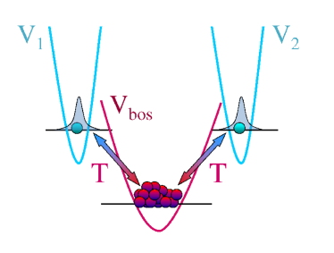
Figure 1: Two atomic qubits coupled to a finite number of cold interacting bosons. The qubits are trapped by the tight potentials $V_{1}$ and $V_{2}$, the bosons are confined in an external potential $V_{bos}$. $T$ is the optical transition assisted coupling between the qubits and the bosons.

Finally, the interaction between the qubits and interacting bosons in the pool reads

$$H_{mix}=T\left[a\sigma_{+}(1)+a^{\dagger}\sigma_{-}(1)+a\sigma_{+}(2)+a^{\dagger}\sigma_{-}(2)\right],$$ (4)

where $a^{\dagger}$ ($a$) creates (annihilates) a boson in the pool and the coupling $T$ is proportional to the Rabi frequency $\Omega_{R}$ of the above-mentioned Raman transition, i.e., $T\sim\hbar\Omega_{R}$. We consider a closed system and the total particle number $N=n+\frac{1}{2}(1+\sigma_{z}(1))+\frac{1}{2}(1+\sigma_{z}(2))$ is conserved, i.e., $[H,N]=0$. In the following we tackle the problem of the dynamics of entanglement in this tripartite system.

III A single AQD coupled to the pool: Bipartite entanglement

It is instructive to start from an even simpler bipartite case of only one AQD coupled to the pool of bosons. Due to the particle number conservation the corresponding Hilbert space $\mathcal{H}=\mathcal{H}_{bos}\otimes\mathcal{H}_{AQD}$ is spanned just by two orthonormal states

$$|n,0\rangle = |n\rangle\otimes|0\rangle,$$

$$|n-1,1\rangle = |n-1\rangle\otimes|1\rangle.$$ (5)

The state $|0\rangle$ corresponds to “spin-down” state of a dot, while the state $|1\rangle$ corresponds to a “spin-up”. The wave function in this case is

$$|\Psi(t)\rangle=c_{1}(t)|n,0\rangle+c_{2}(t)|n-1,1\rangle$$ (6)

with the normalized coefficients $|c_{1}(t)|^{2}+|c_{2}(t)|^{2}=1$. The wave function (6) is in fact equivalent to a standard wave function of two spins-1/2 or two qubits, with two of the four coefficients equal to zero from the onset. We can immediately write down the time-dependent concurrence $C(t)$ of the state as $C(t)=2|c_{1}(t)c_{2}(t)|$ and use it in the following as an entanglement measure Wootters98 . The state is entangled whenever both coefficients $c_{1}$ and $c_{2}$ are nonzero. Note that the initial state $|\Psi(0)\rangle=|n,0\rangle$ is always unentangled.

The Hamiltonian in the basis (5) reads

$$H_{1}=H^{\prime}_{1}\hat{I}_{2}+\left(\begin{array}[]{cc}0&T\sqrt{n}\cr T\sqrt{n}&\quad-E-U(n-1)\end{array}\right),$$ (7)

where $H^{\prime}_{1}=E_{b}n+\frac{1}{2}Un(n-1)$ is the diagonal part of the Hamiltonian (which we neglect in the further consideration) and $E\equiv E_{b}+\Delta$ is the energy difference between the traps. The Hamiltonian (7) describes a two-level system with Rabi frequency $\omega_{R}=T\sqrt{n}$ and detuning $\delta=\frac{1}{2}[-E-U(n-1)]$, so that the eigenenergies are $E_{\pm}=\delta\pm\sqrt{\delta^{2}+\omega_{R}^{2}}$. We note that for $\delta=0$ the ground state is a singlet and the excited state is a triplet.

We now consider the time evolution of the concurrence $C(t)$, or equivalently, the entanglement of the state (6), initially unentangled $|\Psi(0)\rangle=|n,0\rangle$. First, we discuss the case of small detuning $\delta/T\ll 1$. The maximum concurrence is then always close to unity and the concurrence is approximately described by $C\sim|\exp(-2i\delta t)\sin(2\sqrt{n}t)|$, shown in Fig. 2(a) for various $U/T$ and fixed $E$ and $n$. In order to analyze the results, we introduce a convenient quantity $t_{ent}$ referred to as ”entanglement period”, which is the time span between two subsequent instances of zero entanglement. In Fig. 2(a), for example, $t_{ent}=0.5$ for $U/T=0$ and $t_{ent}=1$ for any finite $U/T$ (time is in the units of $1/T$).

In Fig. 2 (b) we plot the entanglement period and the maximum concurrence $C_{max}$ as a function of the interaction $U/T$ for two values of $n$. We see from the results in Fig. 2 (b) in order to increase the entanglement period and maximally possible entanglement one should either decrease $U/T$ or the number of particles in the bosonic pool $n$. Large values of $n$ as well as large values of $U/T$ do not generally advocate entanglement in the system. This happens because the amplitude of the Rabi oscillations scales as $\omega_{R}/(\omega_{R}^{2}+\delta^{2})$, so that large values of $\delta$ contribute to the suppression of entanglement.

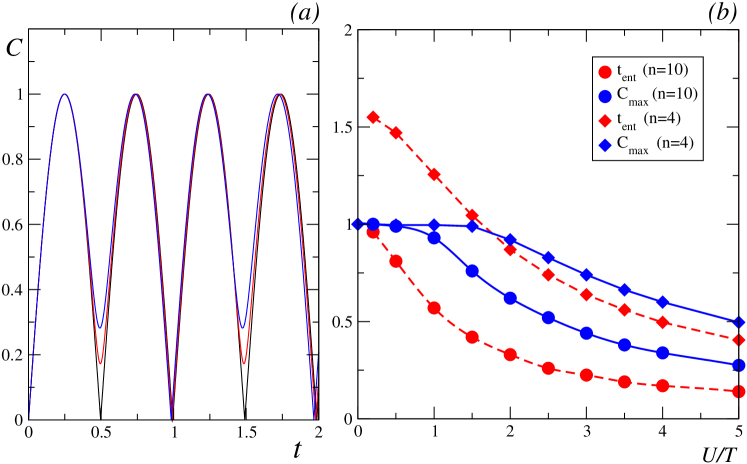
Figure 2: (a) Time evolution of the concurrence of the bipartite setup for $n=10$, $E/T=0.01$ and the interaction $U/T=0$ (black), $U/T=0.06$ (red) and $U/T=0.1$ (blue). (b) Dependence of the entanglement period $t_{ent}$ (red curves) and maximum concurrence $C_{max}$ (blue curves) on the interaction $U/T$ for n=10 (circles) and n=4 (diamonds) bosons in the pool.

IV Two AQDs coupled to the pool: Bipartite and tripartite entanglement

We consider now our initial tripartite system: two AQDs coupled to the pool of interacting bosons. The corresponding Hilbert space is a tensor product of three subspaces $\mathcal{H}=\mathcal{H}_{bos}\otimes\mathcal{H}_{AQD_{1}}\otimes\mathcal{H}_{AQD_{2}}$ and is spanned only by four basis vectors (because of particle conservation) which we choose in the following way

$$\{|n+1,00\rangle,|n,01\rangle,|n,10\rangle,|n-1,11\rangle\}.$$ (8)

Note that the pool is effectively a three state system, i.e., a qutrit, described by the states “spin-up” $|n+1\rangle$, “spin-flat” $|n\rangle$ and “spin-down” $|n-1\rangle$.

We can now write the Hamiltonian of the tripartite system in the basis (8) as

$$H=H_{0}\hat{I}_{4}+\left(\begin{array}[]{cccc}E+Un&T\sqrt{n+1}&T\sqrt{n+1}&0\cr T\sqrt{n+1}&0&0&T\sqrt{n}\cr T\sqrt{n+1}&0&0&T\sqrt{n}\cr 0&T\sqrt{n}&T\sqrt{n}&-E+U(1-n)\end{array}\right),$$ (9)

where $H_{0}=E_{b}n+\frac{1}{2}Un(n-1)-\Delta$ is the diagonal part. One of the eigenstates of this Hamiltonian is a singlet in the AQD sector $|\Psi_{s}\rangle=\frac{1}{\sqrt{2}}|n\rangle\otimes\left(|01\rangle-|10\rangle\right)$ corresponding to an eigenvalue equal to zero. All other eigenvalues have to be determined numerically from the matrix (9). We just mention that the singlet is the second excited state, which is very close to the third excited state (the closer the smaller the interaction energy $U$ is). The ground state and the third excited state are widely separated, the interlevel spacing being proportional to $2\sqrt{n}$ for small $E/T$ and $U/T$.

IV.1 Tripartite entanglement between the AQDs and the pool

We will now turn to the issue of entanglement generation in the tripartite system. The tripartite system is described by the pure state

$$|\Psi\rangle=c_{1}|n+1,00\rangle+c_{2}|n,01\rangle+c_{3}|n,10\rangle+c_{4}|n-1,11\rangle$$ (10)

where $c_{i}(t)$ are complex coefficient satisfying $\sum_{i=1}^{4}|c_{i}(t)|^{2}=1$. Although an entanglement measure is not unambiguously defined for a tripartite hybrid system (one qutrit and two qubits) one can calculate a concurrence Fei

$$C(|\Psi\rangle)=\sqrt{3-\sum_{i=1}^{3}\mbox{Tr}\rho_{i}^{2}}.$$ (11)

where $\rho_{i}$ is the density matrix of a subsystem $i$ with the two other subsystems traced out. The system is unentangled if this concurrence is zero, and a maximum of the concurrence corresponds to the entanglement maximum. We obtain from our full density matrix $\rho=|\Psi\rangle\langle\Psi|$ the three reduced density matrices

$$\rho_{1} = |c_{1}|^{2}|n+1\rangle\langle n+1|+(|c_{2}|^{2}+|c_{3}|^{2})|n\rangle\langle n|+|c_{4}|^{2}|n-1\rangle\langle n-1|,$$ (12)

$$\rho_{2} = (|c_{1}|^{2}+|c_{2}|^{2})|0\rangle\langle 0|+(|c_{3}|^{2}+|c_{4}|^{2})|1\rangle\langle 1|,$$ (13)

$$\rho_{3} = (|c_{1}|^{2}+|c_{3}|^{2})|0\rangle\langle 0|+(|c_{2}|^{2}+|c_{4}|^{2})|1\rangle\langle 1|,$$ (14)

where $\rho_{1}$, $\rho_{2}$ and $\rho_{3}$ are the reduced density matrices of the pool of bosons, the left AQD and the right AQD, respectively. The resulting concurrence (11) reads

$$C(|\Psi\rangle)=\sqrt{3-3\sum_{i=1}^{4}|c_{i}|^{4}-2\left(|c_{2}|^{2}|c_{3}|^{2}+|c_{2}|^{2}|c_{4}|^{2}+|c_{1}|^{2}|c_{2}|^{2}+|c_{1}|^{2}|c_{3}|^{2}+|c_{3}|^{2}|c_{4}|^{2}\right)}\>.$$ (15)

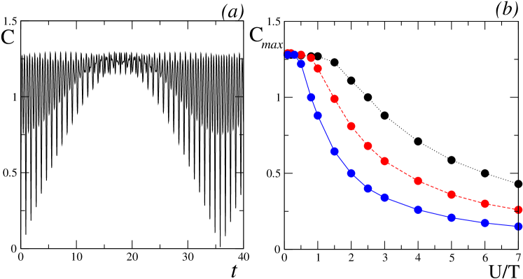
Figure 3: (a) Time-dependent concurrence $C$ of the tripartite setup for $E/T=0.01$, $n=10$ and interaction $U/T=0.2$. (b) The maximum value of concurrence $C_{max}$ of the tripartite system versus interaction $U/T$ for $n=4$ (black), $n=10$ (red) and $n=30$ (blue) bosons in the pool.

In Fig. 3 (a) we display an example of the time-dependent concurrence $C$ for $U/T=0.2$. The initial condition for Fig. 3 and the rest of the plots in the paper is $c_{1}(0)=1$, which corresponds to two initially empty quantum dots. As expected, the time dependence of the concurrence is more complicated than for the bipartite case. However, it is again possible to identify an entanglement period and the maximum concurrence over that period. Note that the maximum concurrence is larger than $1$, which is not surprising since our system comprises a qutrit—a quantum particle with a larger entanglement capacitance than a qubit. In Fig. 3 (b) we plot the maximum concurrence versus interaction $U/T$ for various $n$. We observe similar tendencies as in the previous bipartite case. The maximum concurrence is suppressed by increasing either the interaction or the number of bosons in the pool.

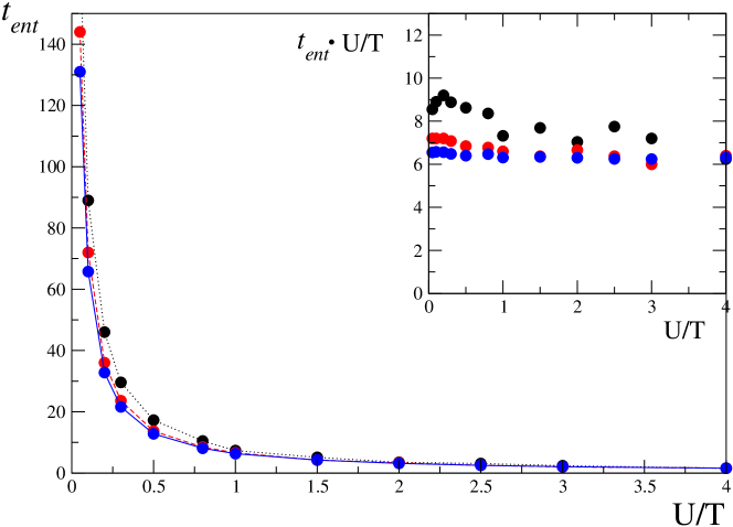
Figure 4: Entanglement period $t_{ent}$ versus interaction for $n=4$ (black), $n=10$ (red) and $n=30$ (blue) interacting bosons in the pool. The product $t_{ent}U/T$ versus $U/T$ is shown in the inset.

Figure 4 shows the dependence of the entanglement period $t_{ent}$ on the bosonic interaction; it is rather different from the bipartite case (see Fig. 2(b)). Importantly, for small $U/T$ the entanglement period can reach values orders of magnitude larger than in the bipartite case, so that the system remains entangled over extended periods of time. We also note that for sufficiently large $n$ the dependence of $t_{ent}$ on the interaction scales approximately as $1/U$, so that $t_{ent}U/T\approx\mathrm{const}$ (see the inset in Fig. 4). Note that because of the units of $t_{ent}$, the product $t_{ent}U/T$ is $T$-independent.

Next we determine the bipartite entanglement in the system when one constituent of the tripartite system is traced out. Entanglement measures for mixed bipartite systems are well defined. In particular, we use the entanglement of formation and the negativity to quantify the entanglement in the bipartite system.

IV.2 Bipartite entanglement between the AQDs

To start with, we trace out the bosonic pool and consider a mixed two qubit state described by the reduced density matrix

$$\rho_{1}=\left(\begin{array}[]{cccc}|c_{1}|^{2}&0&0&0\cr 0&|c_{2}|^{2}&c_{2}c_{3}^{*}&0\cr 0&c_{3}c_{2}^{*}&|c_{3}|^{2}&0\cr 0&0&0&|c_{4}|^{2}\end{array}\right)$$ (20)

written in a standard two-qubit basis. Entanglement of formation $E_{f}$ can be defined in this case as Wootters98

$$E_{f}(\rho_{1})=f\left(\frac{1+\sqrt{1-C(\rho_{1})^{2}}}{2}\right)$$ (21)

with $f(x)=-x\log_{2}x-(1-x)\log_{2}(1-x)$, and the concurrence

$$C(\rho_{1})=max\{0,\lambda_{1}-\lambda_{2}-\lambda_{3}-\lambda_{4}\}.$$ (22)

Here, $\lambda_{i}$ are the square roots of the eigenvalues of $\rho_{1}\tilde{\rho}_{1}$ in descending order, where $\tilde{\rho}_{1}=(\sigma_{y}\otimes\sigma_{y})\rho_{1}^{*}(\sigma_{y}\otimes\sigma_{y})$, and $\rho_{1}^{*}$ is a complex conjugate of $\rho_{1}$. After some algebra we obtain $\lambda_{1}=0,\lambda_{2,3}=|c_{1}||c_{4}|$ and $\lambda_{4}=2|c_{2}||c_{3}|$, which have still to be ordered. This allows us to calculate the concurrence and the corresponding entanglement of formation according to (21).

An alternative measure of entanglement is the negativity Werner02

$$\mathcal{N}(\rho_{1})=\frac{||\rho_{1}^{\Gamma}||_{1}-1}{2}\,.$$ (23)

Here, $||\rho_{1}^{\Gamma}||_{1}$ is the trace norm of the partial transpose $\rho_{1}^{\Gamma}$ of the bipartite mixed state. Essentially $\mathcal{N}(\rho_{1})$ is just the absolute value of the sum of negative eigenvalues of $\rho_{1}^{\Gamma}$. After some algebra we find that only the eigenvalue $\lambda=(|c_{1}|^{2}+|c_{4}|^{2}-\sqrt{(|c_{1}|^{2}-|c_{4}|^{2})+4|c_{2}|^{2}|c_{3}|^{2}})/2$ of the partial transpose of the density matrix (20) can be negative.

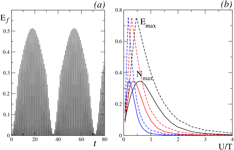
Figure 5: (a) Time dependence of the entanglement of formation $E_{f}$ for $U/T=0.2$ and $n=10$. (b) The maximum values of the entanglement of formation $E_{max}$ (dashed curves) and the negativity $N_{max}$ (solid curves) versus the interaction $U/T$ for $n=4$ (black), $n=10$ (red) and $n=30$ (blue) bosons in the pool.

The periodic time dependence of the entanglement of formation is presented in Fig. 5. We note that the entanglement of formation and negativity have the same time dependence, however, they are different in amplitude, which is not surprising since the entanglement of formation and negativity are different entanglement measures Verstraete ; Wei . We therefore analyze the dependence of the maximal entanglement of formation $E_{max}$ and maximal negativity $N_{max}$ on the interaction energy $U/T$. The results for different boson numbers $n$ are shown in Fig. 5(b).

An unexpected result is that the curves $E_{max}(U)$ and $N_{max}(U)$ are nonmonotonic. Each curve possesses a maximum at a characteristic value of $U=U_{c}$. The value of $U_{c}$ depends on the number of bosons $n$, more precisely, $U_{c}$ is increasing with decreasing $n$; on the other hand, the $E_{max}(U_{c})$ and $N_{max}(U_{c})$ are constant. The nonmonotonic behavior of the curves is probably related to the fact that for $U/T\ll 1$ the main entanglement capacity resides in the bosonic reservoir, which is traced out in the case at hand. Indeed, when just one ADQ is traced out instead, we observe a monotonic dependence (see next section).

IV.3 Bipartite entanglement between a single AQD and the pool

Finally, we trace out one of the qubits and discuss entanglement of the hybrid qubit-qutrit system described by the reduced density matrix

$$\rho_{2}=\left(\begin{array}[]{cccc}|c_{1}|^{2}&c_{1}c_{2}^{*}&0&0\cr c_{1}^{*}c_{2}&|c_{2}|^{2}&0&0\cr 0&0&|c_{3}|^{2}&c_{3}c_{4}^{*}\cr 0&0&c_{3}^{*}c_{4}&|c_{4}|^{2}\end{array}\right).$$ (28)

In order to determine the negativity we again need to find negative eigenvalues of the partial transpose of the density matrix (28). It turns out that only two eigenvalues can be negative, namely $\lambda_{1}=(|c_{2}|^{2}-\sqrt{|c_{2}|^{4}+4|c_{3}|^{2}|c_{4}|^{2}})/2$ and $\lambda_{2}=(|c_{3}|^{2}-\sqrt{|c_{3}|^{4}+4|c_{1}|^{2}|c_{2}|^{2}})/2$. We can now calculate the negativity as an absolute sum of negative eigenvalues of $||\rho_{2}^{\Gamma}||_{1}$ (see previous section).

The entanglement of formation can be also calculated by doing a convex expansion of the density matrix $\rho_{2}$ Wootters01 :

$$\rho_{2}=\alpha\rho_{\alpha}+\beta\rho_{\beta}=\alpha|\Psi_{\alpha}\rangle\langle\Psi_{\alpha}|+\beta|\Psi_{\beta}\rangle\langle\Psi_{\beta}|,$$ (29)

whereby the pure states $|\Psi_{\alpha}\rangle$ and $|\Psi_{\beta}\rangle$ are

$$|\Psi_{\alpha}\rangle=\frac{1}{\sqrt{\alpha}}\left(c_{1}|n+1,0\rangle+c_{2}|n,1\rangle\right),$$ (30)

$$|\Psi_{\beta}\rangle=\frac{1}{\sqrt{\beta}}\left(c_{3}|n,0\rangle+c_{4}|n-1,1\rangle\right).$$ (31)

Here, $\alpha=|c_{1}|^{2}+|c_{2}|^{2}$ and $\beta=|c_{3}|^{2}+|c_{4}|^{2}$, so that $\alpha+\beta=1$. One should note that the decomposition (29) is unique because of the prohibition against superpositions of states with different particle numbers. The resultant entanglement of formation is Wootters01

$$E=\alpha E_{\alpha}+\beta E_{\beta},$$ (32)

where $E_{{\alpha}(\beta)}$ is the entanglement of formation of the state $|\Psi_{\alpha}\rangle$ ($|\Psi_{\beta}\rangle$) calculated with corresponding concurrencies $C_{\alpha}=2|c_{1}c_{2}|/\alpha$ and $C_{\beta}=2|c_{3}c_{4}|/\beta$.

Figure 6 shows the entanglement of formation $E_{f}$ versus time for a fixed interaction strength; the dependence of the negativity is similar up to a scaling factor. In Fig. 6(b) the maximum entanglement of formation $E_{max}$ and maximum negativity $N_{max}$ are plotted versus interaction $U/T$ for different bosonic occupations. The behavior of these quantities is monotonic and in line with the $U/T$-dependence of the maximum concurrence shown in Fig. 3(b): Smaller boson numbers $n$ in the pool favor larger values of entanglement.

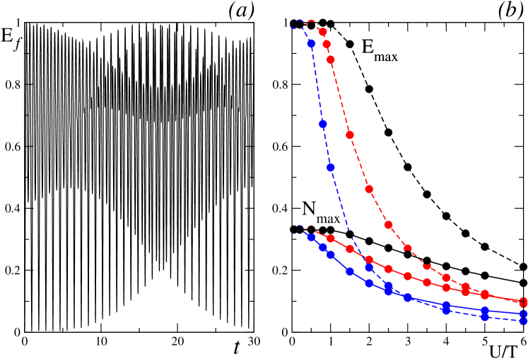
Figure 6: (a) Time dependence of the entanglement of formation $E_{f}$ for $U/T=0.2$ and $n=10$. (b) The maximum values of the entanglement of formation $E_{max}$ (dashed curves) and the negativity $N_{max}$ (solid curves) versus interaction $U/T$ for $n=4$ (black), $n=10$ (red) and $n=30$ (blue) bosons in the pool.

V Conclusions and discussions

We have analyzed qubit-qubit, qubit-qutrit and qubit-qutrit-qubit systems which can be realized in a cold atomic set-up. Qutrits have bigger entanglement capacity and offer potentially more advantages for quantum computation than qubits. However, they are difficult to handle, as they involve more degrees of freedom. Qubit-qutrit entanglement has been recently observed for the first time in a photonic system Nathan . Cold atomic qutrits, which emerge due to the particle conservation, are characterized by the number of bosons and their interactions; both parameters can be easily tuned experimentally.

We have demonstrated that both parameters play a crucial role in generating the maximal possible entanglement between the subsystems as well as for the longest entanglement period. For example, smaller number of particles and smaller interactions in general favor the generation of entanglement. Note that increasing $n$ ($n\gg 1$) leads to the disappearance of entanglement as expected EPL . Systems with large interactions ($U/T\gg 1$) do not exhibit entanglement. Interestingly, the entanglement period of the tripartite system is orders of magnitude larger than that of the bipartite system. We have also found a simple relation between entanglement period and interaction for large number of bosons ($n\gg 1$).

Note that in this work we dealt with so-called mode entanglement Zanardi , i.e., entanglement of modes in the Fock representation. It was debated whether or not mode entanglement can be effectively used for quantum computatiom because superselection rules prohibit coherent superpositions of different particle number, which introduces severe limitations. However, it has been shown recently that there are ways to overcome this drawback, for example, mode entanglement can be used for dense coding Vedral .

Our results may also shed light on the role played by interactions in the problem of coupled harmonic oscillators Osc . One can assume from our findings that entanglement between oscillators strongly depends on the ratio of interaction versus coupling. Another interesting extension our results could be the study of entanglement between atomic Bose-Einstein condensates and immersed impurities Koehl ; Johnson .

Acknowledgments We are grateful to M. Eschrig, D. Jaksch, N. Langford, G.J. Milburn, and W. K. Wootters for fruitful and valuable comments and discussions. W.B. acknowledges financial support from the German Research Foundation (DFG) through SFB 767 and SP 1285.

References

- (1) M. A. Nielsen and I. L. Chuang, Quantum Computation and Quantum Information (Cambridge Univ. Press, 2000).
- (2) C. H. Bennett and S. J. Wiesner, Phys. Rev. Lett. 69, 2881 (1992).
- (3) C. H. Bennett, G. Brassard, C. Crepeau, R. Jozsa, A. Peres, and W. K. Wootters, Phys. Rev. Lett. 70, 1895 (1993).
- (4) L. Amico, R. Fazio, A. Osterloh, and V. Vedral, Rev. Mod. Phys. 80, 517 (2008).
- (5) J. Bardeen, L. N. Cooper, and J. R. Schrieffer, Phys. Rev. 108, 1175 (1957).
- (6) R. B. Laughlin, Phys. Rev. Lett. 50, 1395 (1983).
- (7) A. Hewson, The Kondo Problem to Heavy Fermions, Cambridge University Press, Cambridge, England (1997).
- (8) A. Osterloh, L. Amico, G. Falci, and R. Fazio, Nature (London) 416, 608 (2002).
- (9) G. Vidal, J. I. Latorre, E. Rico, and A. Kitaev, Phys. Rev. Lett. 90, 227902 (2003).
- (10) G. Refael and J. E. Moore, Phys. Rev. Lett. 93, 260602 (2004).
- (11) A. Kitaev and J. Preskill, Phys. Rev. Lett. 96, 110404 (2006).
- (12) M. Levin and X.-G. Wen, Phys. Rev. Lett. 96, 110405 (2006).
- (13) O. Mandel, M. Greiner, A. Widera, T. Rom, T. W Hänsch, and I. Bloch, Nature 425, 937 (2003).
- (14) D. Jaksch, H. J. Briegel, J.I. Cirac, C. W. Gardiner, and P. Zoller, Phys. Rev. Lett. 82, 1975 (1999).
- (15) S. R. Clark, C. Moura Alves, and D. Jaksch, New J. Phys. 7, 124 (2005).
- (16) S. R. Clark, A. Klein, M. Bruderer, and D. Jaksch, New J. Phys. 9, 202 (2007).
- (17) L. Banchi, A. Bayat, P. Varrucchi, and S. Bose, Phys. Rev. Lett. 106, 140501 (2011).
- (18) W. S. Bakr, A. Peng, M. E. Tai, R. Ma, J. Simon, J. I. Gillen,. S. Fölling, L. Pollet, and M. Greiner, Science 329, 547 (2010).
- (19) J. F. Sherson, C. Weitenberg, M. Endres, M. Cheneau, I. Bloch, and S. Kuhr, Nature 467, 68 (2010).
- (20) K. A. Dennison and W. K. Wootters, Phys. Rev. A 65, 010301(R) (2001).
- (21) W. K. Wootters, Phys. Rev. Lett. 80, 2245 (1998).
- (22) G. Vidal, R. F. Werner, Phys. Rev. A 65, 032314 (2002).
- (23) A. Posazhennikova and W. Belzig, Eur. Phys. Lett. 87, 56004 (2009).
- (24) D. Jaksch, C. Bruder, J. I. Cirac, C. W. Gardiner, P. Zoller, Phys. Rev. Lett. 81, 3108 (1998).
- (25) A. Recati, P. O. Fedichev, W. Zwerger, J. von Delft, and P. Zoller, Phys. Rev. Lett. 94, 040404 (2005).
- (26) S. Zippilli, and G. Morigi, Phys. Rev. Lett. 95, 143001 (2005).
- (27) X.-H. Gao, S.-M. Fei, Eur. Phys. J. Special Topics 159, 71 (2008).
- (28) F. Verstraete, K. Audenaert, J. Dehaene, and B. De Moor, J.Phys.A: Math. Gen. 34, 10327 (2001).
- (29) T. C. Wei, K. Nemoto, P. M. Goldbart, P. G. Kwiat, W. J. Munro, and F. Verstraete, Phys. Rev. A 67, 022110(2003).
- (30) W. K. Wootters, Quantum Information and Computation 1, 27 (2001).
- (31) B. P. Lanyon, T. J. Weinhold, N. K. Langford, J. L. O’Brien, K.J. Resch, A. Gilchrist, and A. G. Whie, Phys. Rev. Lett. 100, 060504 (2008).
- (32) P. Znardi, Phys. Rev. A 65, 042101 (2002).
- (33) L. Heaney and V. Vedral, Phys. Rev. Lett. 103, 200502 (2009).
- (34) K. Audenaert, J. Eisert, M. B. Plenio, and R. F. Werner, Phys. Rev. A 66, 042327 (2002).
- (35) C. Zipkes, S. Palzer, C. Sias, and M. Köhl, Nature 464, 388 (2010).
- (36) T. H. Johnson, S. R. Clark, M. Bruderer, and D. Jaksch, Phys. Rev. A 84 023617 (2011).