Critical behavior of a water monolayer under hydrophobic confinement

The properties of water can have a strong dependence on the confinement. Here, we consider a water monolayer nanoconfined between hydrophobic parallel walls under conditions that prevent its crystallization. We investigate, by simulations of a many-body coarse-grained water model, how the properties of the liquid are affected by the confinement. We show, by studying the response functions and the correlation length and by performing finite-size scaling of the appropriate order parameter, that at low temperature the monolayer undergoes a liquid-liquid phase transition ending in a critical point in the universality class of the two-dimensional (2D) Ising model. Surprisingly, by reducing the linear size $L$ of the walls, keeping the walls separation $h$ constant, we find a 2D-3D crossover for the universality class of the liquid-liquid critical point for $L/h\simeq 50$, i.e. for a monolayer thickness that is small compared to its extension. This result is drastically different from what is reported for simple liquids, where the crossover occurs for $L/h\simeq 5$, and is consistent with experimental results and atomistic simulations. We shed light on these findings showing that they are a consequence of the strong cooperativity and the low coordination number of the hydrogen bond network that characterizes water.


PACS number 64.70.Ja, 65.20.-w, 68.15.+e

The study of nanoconfined water is of great interest for applications in nanotechnology and nanoscience majumder . The confinement of water in quasi-one or two dimensions (2D) is leading to the discovery of new and controversial phenomena in experiments majumder ; Whitby2007 ; Zhang2011 ; soper ; han2010 and simulations Whitby2007 ; faraudo-bresme ; shr . Nanoconfinement, both in hydrophilic and hydrophobic materials, can keep water in the liquid phase at temperatures as low as 130 K at ambient pressure Zhang2011 . At these temperatures $T$ and pressures $P$ experiments cannot probe liquid water in the bulk, because water freezes faster then the minimum observation time of usual techniques, resulting in an experimental “no man’s land” Mishima1998 . Nevertheless, new kind of experiments nillson1 ; taschin and numerical simulations llcp can access this region, revealing interesting phenomena in the metastable state. In particular, Poole et al. found, by molecular dynamics simulations of supercooled water, a liquid-liquid critical point (LLCP), in the “no man’s land”, at the end of a first–order liquid-liquid phase transition (LLPT) line between two metastable liquids phases with different density $\rho$: the high-density liquid (HDL) at higher $T$ and $P$, and the low-density liquid (LDL) at lower $T$ and $P$ llcp . The presence of a LLPT is experimentally observed in other systems anomalous-exp ; exp1 ; exp2 ; exp3 ; exp4 ; exp5 ; exp6 ; exp7 ; exp8 ; mcmillan , consistent with theoretical models fitted to water experimental data Anisimov ; holten1 ; nillson2 , and is recovered by simulations of a number of models of water llcp ; LLCPnew ; llcp1 ; llcp2 ; llcp3 ; llcp4_bis ; llcp5 ; FMS2003 and other anomalous liquids anomalous-sim ; an1 ; an2 ; an3 ; an7 ; an8 . Alternative ideas, and their differences, have been discussed sf ; Stokely2010 ; Limmer ; llcp4 ; palmer , and it has been debated if experiments on confined water in the “no man’s land” can be a way to test these ideas Zhang2011 , motivating several theoretical works gallo-rovere .

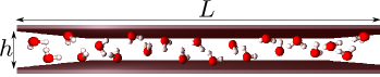
Figure 1: Schematic view of a section of the water monolayer confined between hydrophobic walls of size $L\times L$ separated by $h\approx 0.5$ nm.

Here, to analyze the thermodynamic properties of water in confinement we consider a water monolayer between hydrophobic walls of area $L^{2}$ separated by $h\approx 0.5$ nm (Fig. 1). Atomistic simulations shr show that water under these conditions does not crystallize, but arranges in a disordered liquid layer, whose projection on one of the surfaces has square symmetry, with each water molecule having four nearest neighbors (n.n.). The molecules maximize their intermolecular distance by adjusting at different heigths with respect to the two walls.

We adopt a many-body model that reproduces water properties FMS2003 ; Stokely2010 ; KFS2008 ; dls ; MSSSF2009 ; bb ; bbb ; Mazza ; fbfood2013 . We simulate $\sim 10^{5}$ state points, each with statistics of $5\times 10^{6}$ independent calculations, for systems with $N=2.5\times 10^{3},\dots,1.6\times 10^{5}$ water molecules at constant $N$, $P$ and $T$, using a cluster Monte Carlo algorithm MSSSF2009 ; bb ; bbb , for a wide range of $T$ and $P$. All quantities are calculated in internal units, as described in the Methods section.

Results

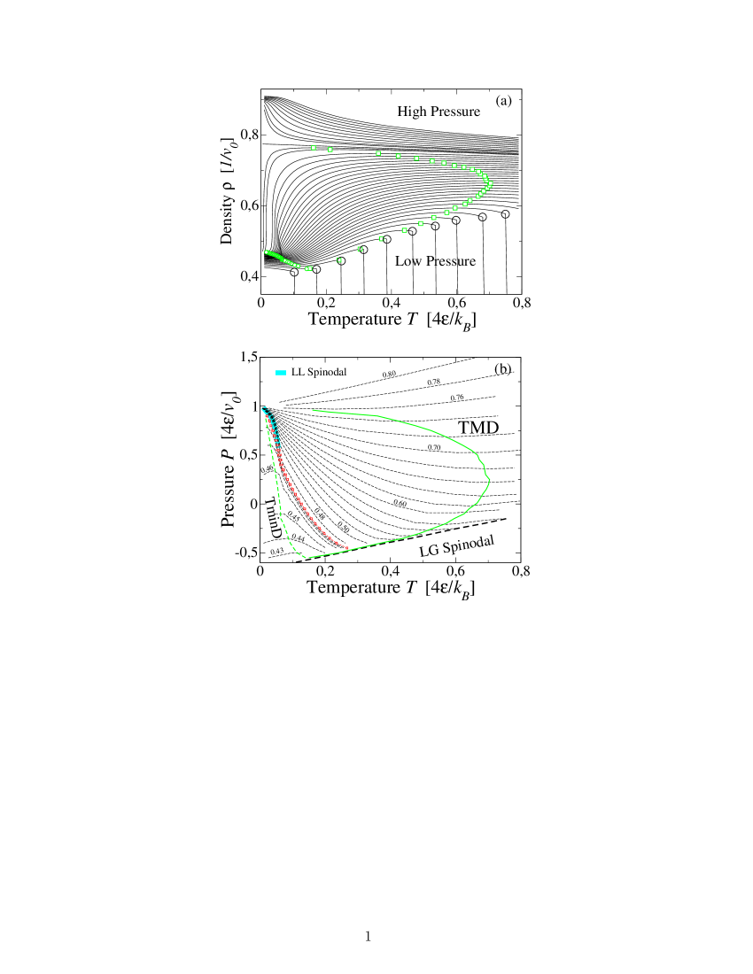
Figure 2: (a) Isobaric density variation for $10^{4}$ water molecule. Lines join simulated state points ($\sim 150$ for each isobar). $P$ increases from $-0.5$ (bottom curve) to $1.5$ $(4\epsilon)/v_{0}$ (top curve). Along each isobar we locate the maximum $\rho$ (green squares at high $T$) and the minimum $\rho$ (green small circles at low $T$) and the liquid-gas spinodal (open large circles at low $P$). (b) Loci of TMD, TminD, liquid-gas spinodal and liquid-liquid spinodal in $T-P$ plane. Dashed lines with labels represent the isochores of the system from $\rho v_{0}=0.43$ (bottom) to $\rho v_{0}=0.80$ (top). Dashed lines without labels represent intermediate isochores. TMD and TminD correspond to the loci of minima and maxima, respectively, along isochores in the $T-P$ plane. We estimate the critical isochore at $\rho v_{0}\sim 0.47$ (red circles). All the isochores with $0.47<\rho v_{0}<0.76$ intersect with the critical isochore for $Pv_{0}/(4\epsilon)\geq 0.5$ along the LL spinodal (tick turquoise) line.

We calculate the density $\rho\equiv N/V$ of the system as function of $T$ along isobars. For a broad range of $P$, we find a maximum and a minimum of density along each isobar (Fig. 2a) according to experimental evidences for bulk and confined water Mallamace-density-min . These maxima and minima identify, for each $P$, the temperature of maximum density (TMD) and the temperature of minimum density (TminD). The TMD locus merges the TminD line as in experiments Mallamace-density-min and other models Poole2005 .

At low $T$ a discontinuous change in $\rho$ is observed for $1>Pv_{0}/(4\epsilon)\geq 0.5$, where the parameters $v_{0}$ and $\epsilon$ are explained in the Methods section, as it would be expected in correspondence of the HDL-LDL phase transition. At very high pressures ($Pv_{0}/(4\epsilon)>1$) the system behaves as a normal liquid, with monotonically increase of $\rho$ upon decrease of $T$.

We estimate the liquid-to-gas (LG) spinodal at $Pv_{0}/(4\epsilon)<0$ for low $T$ (Fig. 2) as the temperature along an isobar at which we find a discontinuous jump of $\rho$ to zero value by heating the system. The LG spinodal identifies the locus of the stability limit of liquid phase with respect to the gas phase: at pressures below the LG spinodal in the $P-T$ plane is no longer possible to equilibrate the system in the liquid phase. The LG spinodal continues at positive pressures ending in the LG critical point (data not shown). We observe that the TMD line approaches the LG spinodal, without touching it (Fig. 2). We recover the LG spinodal also as envelope of isochores (Fig. 2b).

We find a second envelope of isochores at lower $T$ and higher $P$, pointing out the liquid-to-liquid (LL) spinodal. Indeed, the two spinodals associated to the LLPT, i.e. the HDL-to-LDL spinodal and the LDL-to-HDL spinodal, collapse one on top of the other and are indistinguishable within our numerical resolution. Nevertheless, we clearly see that isochores are gathering around the points ($Tk_{B}/(4\epsilon)\sim 0.06$, $Pv_{0}/(4\epsilon)\sim 0.5$ ) and ($Tk_{B}/(4\epsilon)=0$, $Pv_{0}/(4\epsilon)=1$), where $k_{B}$ is the Boltzmann constant, marking two possible critical regions (Fig. 2b).

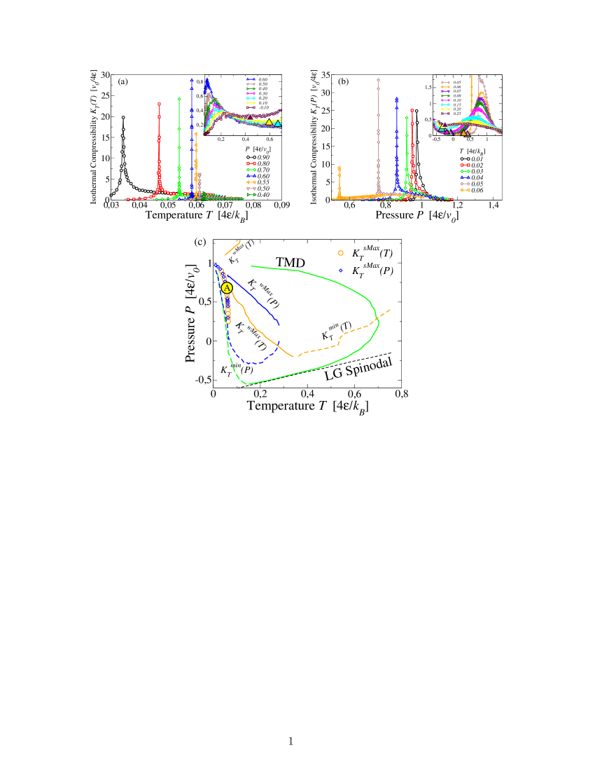
Figure 3: (a) Loci of strong maxima ($K_{T}^{\rm sMax}(T)$), weak maxima ($K_{T}^{\rm wMax}(T)$ in the inset) and minima ($K_{T}^{\rm min}(T)$ marked with large triangles in the inset) along isobars for $K_{T}(T)$. (b) Loci of strong maxima ($K_{T}^{\rm sMax}(P)$), weak maxima ($K_{T}^{\rm wMax}(P)$ in the inset) and minima ($K_{T}^{\rm min}(P)$ marked with large triangles in the inset) along isotherms. The weak maxima merge with minima. (c) Projection of extrema of $K_{T}$ in $T-P$ plane. The strong maxima (symbols), weak maxima (solid lines) and minima (dashed lines) of $K_{T}(T)$ (orange) and $K_{T}(P)$ (blue) form loci in $T-P$ plane that relate to each other and intersect with the TMD line following the thermodynamic relations discussed in the text. The large yellow circle with label A identifies the region where $K_{T}^{\rm sMax}(T)$ and $K_{T}^{\rm sMax}(P)$ converge and display the largest maxima, consistent with the occurrence of a critical point in a finite-size system. Symbols not explained here are as in Fig. 2.

We calculate the isothermal compressibility by its definition $K_{T}\equiv-(1/\langle V\rangle)\left(\partial\langle V\rangle/\partial P\right)_{T}$ and by the fluctuation-dissipation theorem $K_{T}=\langle\Delta V^{2}\rangle/k_{B}TV$ along isobars, $K_{T}(T)$, and along isotherms, $K_{T}(P)$ (Fig. 3), where $\langle V\rangle\equiv V$ is the average volume and $\langle\Delta V^{2}\rangle$ the volume fluctuations. We find two loci of extrema for each quantity $K_{T}(T)$ and $K_{T}(P)$: one of strong maxima and one of weak maxima. The loci of strong maxima in $K_{T}(T)$ and $K_{T}(P)$, respectively $K_{T}^{\rm sMax}(T)$ and $K_{T}^{\rm sMax}(P)$, overlap within the error bar with the LL spinodal. The maxima $K_{T}^{\rm sMax}(T)$ and $K_{T}^{\rm sMax}(P)$ increase in the range of $Pv_{0}/(4\epsilon)\in[0.55;0.6]$ and $Tk_{B}/(4\epsilon)\in[0.05;0.06]$ (Fig. 3), consistent with the existence of a critical region. The stronger maxima disappear for $Pv_{0}/(4\epsilon)<0.4$.

We find also loci of weak maxima, $K_{T}^{\rm wMax}(T)$ and $K_{T}^{\rm wMax}(P)$ and minima $K_{T}^{\rm min}(T)$ and $K_{T}^{\rm min}(P)$. The loci of weak extrema and minima of $K_{T}(T)$ and $K_{T}(P)$ do not coincide in the $T-P$ plane. The locus of weak maxima along isotherms $K_{T}^{\rm wMax}(P)$ merges with the locus of minima $K_{T}^{\rm min}(P)$ at the point where the slope of both loci is $\partial P/\partial T\rightarrow\infty$. Furthermore, both loci approach to the LL spinodal at high $P$. The locus of weak maxima along isobars $K_{T}^{\rm wMax}(T)$ approaches the LL spinodal where $K_{T}$ exhibits the strongest maxima, and merges with the locus of minima $K_{T}^{\rm min}(T)$ where the slope of both loci is $\partial P/\partial T\rightarrow 0$ (data at high $P$ and $T$ not shown in Fig 3). This locus intersects the TMD at its turning point. Indeed, as reported in Ref. sf and in the Methods section, the temperature derivative of isobaric $K_{T}$ along the TMD line is related to the slope of TMD line

$$\left(\dfrac{\partial K_{T}}{\partial T}\right)_{P,~{}\rm TMD}=\dfrac{1}{V}\dfrac{(\partial^{2}V/\partial T^{2})_{\rm TMD}}{(\partial P/\partial T)_{\rm TMD}}$$ (1)

where all the quantities are calculated along the TMD line. Hence the locus of extrema in $K_{T}(T)$, where $(\partial K_{T}/\partial T)_{P}=0$, crosses the TMD line where the slope $(\partial P/\partial T)_{\rm TMD}$ is infinite. We observe also that the weak maxima of $K_{T}(T)$ and $K_{T}(P)$ increase as they approach the LL spinodal. All loci of extrema in $K_{T}$ are summarized in Fig. 3.

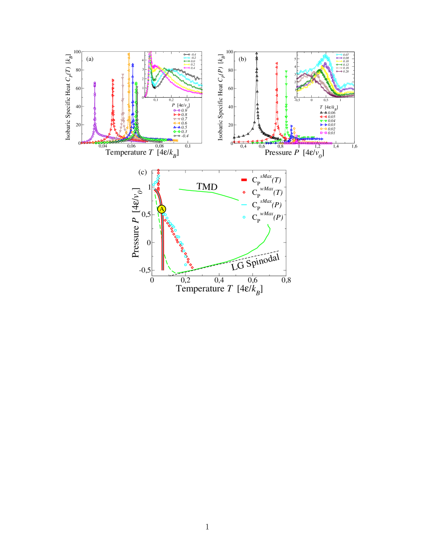
Figure 4: (a) Loci of strong maxima ($C_{P}^{\rm sMax}(T)$) and weak maxima ($C_{P}^{\rm wMax}(T)$ in the inset) along isobars for $C_{P}$. (b) Loci of strong maxima ($C_{P}^{\rm sMax}(P)$) and weak maxima ($C_{P}^{\rm wMax}(P)$ in the inset) along isotherms. (c) Projection of $C_{P}$ maxima in $T-P$ plane. The large circle with A identifies the region where $C_{P}$ shows the strongest maximum. Symbols not explained here are as in Fig. 2.

Next we calculate the isobaric specific heat $C_{P}\equiv\left(\partial\langle H\rangle/\partial T\right)_{P}=\langle\Delta H^{2}\rangle/k_{B}T$ along isotherms and isobars, where $\langle H\rangle\equiv\langle\mathscr{H}\rangle+P\langle V\rangle$ is the average enthalpy, $\mathscr{H}$ is the Hamiltonian as defined in the Methods section, $\langle\Delta H^{2}\rangle$ is the enthalpy fluctuations (Fig. 4). We find two maxima at low $P$ separated by a minimum. At high-$T$ the maxima are broader and weaker than those at low-$T$. As discussed in Ref. Mazza , the maxima at high $T$ are related to maxima in fluctuation of the HB number $N_{\rm HB}$, while the maxima at low $T$ are a consequence of maxima in fluctuations of the number $N_{\rm coop}$ of cooperative HBs. The lines of strong maxima at constant $P$ and constant $T$, respectively $C_{P}^{\rm sMax}(T)$ and $C_{P}^{\rm sMax}(P)$, overlap for all the considered pressures, and both maxima are more pronounced in the range $Pv_{0}/(4\epsilon)\in[0.5,0.6]$ and $Tk_{B}/(4\epsilon)\in[0.06,0.07]$. The weak maxima $C_{P}^{\rm wMax}(P)$ and $C_{P}^{\rm wMax}(T)$ increase approaching the LL spinodal and have their larger maxima at the state point where they converg to the strong maxima, consistent with the occurrence of a critical point for a finite system (Fig. 4). The lines of weak maxima overlap for all positive pressures, branching off at negative pressures. At negative pressures, the locus $C_{P}^{\rm wMax}(P)$ bends toward the turning point of the TMD line, as discussed in Methods section and in Ref. Poole2005 . Indeed, according to the relation

$$\left(\frac{\partial C_{P}}{\partial P}\right)_{T,~{}\rm TMD}=T\left(\frac{\partial P}{\partial T}\right)_{\rm TMD}\left(\frac{\partial^{2}V}{\partial P\partial T}\right)_{\rm TMD},$$ (2)

in case of intersection between the locus of extrema $(\partial C_{P}/\partial P)_{T}=0$ and the TMD line, it results that $(\partial P/\partial T)_{\rm TMD}=0$. Note that, as we explain in the Methods section, the relation (2) does not imply any change in the slope of the TminD line at the intersection with the locus of $(\partial C_{P}/\partial P)_{T}=0$.

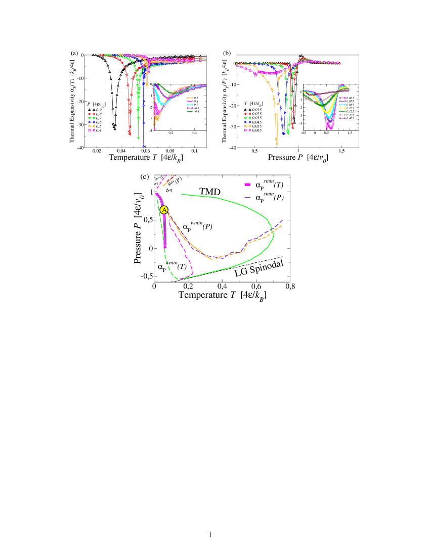
Figure 5: (a) Loci of strong minima of ($\alpha_{P}^{\rm smin}(T)$) and weak minima ($\alpha_{P}^{\rm wmin}(T)$ in the inset) along isobars for $\alpha_{P}$. (b) Loci of strong minima ($\alpha_{P}^{\rm smin}(P)$) and weak extrema ($\alpha_{P}^{\rm Max}(P)$ and $\alpha_{P}^{\rm wmin}(P)$ in the inset) along isotherms. (c) Projection of $\alpha_{P}$ extrema in $T-P$ plane. Orange lines are the loci of weaker extrema $K_{T}^{\rm wMax}$ and $K_{T}^{\rm min}$. The large circle with A identifies the region where the divergent minimum in $\alpha_{P}$ is observed. Symbols not explained here are as in Fig. 2.

We calculate also the thermal expansivity $\alpha_{P}\equiv(1/\langle V\rangle)\left(\partial\langle V\rangle/\partial T\right)_{P}$ along isotherms and isobars (Fig. 5). As for the other response functions, we find two loci of strong extrema, minima in this case, $\alpha_{P}^{\rm smin}(P)$ and $\alpha_{P}^{\rm smin}(T)$, along isotherms and isobars, respectively showing a divergent behavior in the same region where we find the strong maxima of $K_{T}$ and $C_{P}$. From this region two loci of weaker minima depart. We find that the locus of weak minima along isobars $\alpha_{P}^{\rm wmin}(T)$ bends toward the turning point of the TMD. Although our calculations for $\alpha_{P}$ do not allow us to observe the crossing with the TMD line, based on the relation (see Methods)

$$\left(\frac{\partial\alpha_{P}}{\partial T}\right)_{P,~{}\rm TMD}=-\frac{1}{V}\left(\frac{\partial P}{\partial T}\right)_{\rm TMD}\left(\frac{\partial^{2}V}{\partial P\partial T}\right)_{\rm TMD}$$ (3)

that holds at the TMD line, we can conclude that $\alpha_{P}^{\rm wmin}(T)$ should have zero $T$-derivative if it crosses the point where the TMD turns into the TminD line, because in this point the TMD slope approaches zero.

The locus of weaker minima along isotherms $\alpha_{P}^{\rm wmin}(P)$, merges with the locus of maxima $\alpha_{P}^{\rm Max}(P)$ at the state point where the slope of both loci is $\partial P/\partial T\rightarrow\infty$ (not shown in Fig. 5). According to the thermodynamic relation, discussed in Methods section,

$$\left(\dfrac{\partial\alpha_{P}}{\partial P}\right)_{T}=-\left(\dfrac{\partial K_{T}}{\partial T}\right)_{P},$$ (4)

we find that the locus of extrema in thermal expansivity along isotherms coincides, within the error bars, with the locus of extrema of isothermal compressibility along isobars (Fig. 5c).

All the loci of extrema of response functions that converge toward the same region $A$ in Fig. 3, 4 and 5 increase in their absolute values. Because the increase of response functions is related to the increase of fluctuations and this is, in turn, related to the increase of correlation length $\xi$, to estimate $\xi$ we calculate the spatial correlation function

$$G(r)\equiv\dfrac{1}{4N}\sum_{|\vec{r_{i}}-\vec{r_{l}}|=r}\left[\langle\sigma_{ij}(\vec{r_{i}})\sigma_{lk}(\vec{r_{l}})\rangle-\langle\sigma_{ij}\rangle^{2}\right]$$ (5)

where $\vec{r_{i}}$ is the position of the molecule $i$, $|\vec{r_{i}}-\vec{r_{l}}|=r$ the distance between molecule $i$ and molecule $l$ and $\langle\cdot\rangle$ the thermodynamic average. The states of the water molecule, as well as the density $\rho$, the energy $E$ and the entropy $S$ of the system, are completely described by the bonding variables $\sigma_{ij}$. Therefore, the function $G(r)$ accounts for the fluctuations in $\rho$, $E$ and $S$ and allows us to evaluate the correlation length because the order parameter of the LLPT, as we discuss in the following, is related to a linear combination of $\rho$ and $E$. Note that, instead, the density-density correlation function would give only an approximate estimate of $\xi$.

We observe an exponential decay of $G(r)\sim e^{-r/\xi}$ at high temperatures in a broad range of pressures. Approaching the region $A$, the correlation function can be written as $G(r)\sim e^{-r/\xi}/r^{d-2+\eta}$ where $d$ is the dimension of the system and $\eta$ a (critical) positive exponent. When $\xi$ is of the order of the system size, the exponential factor approaches a constant leaving the power-law as the dominant contribution for the decay.

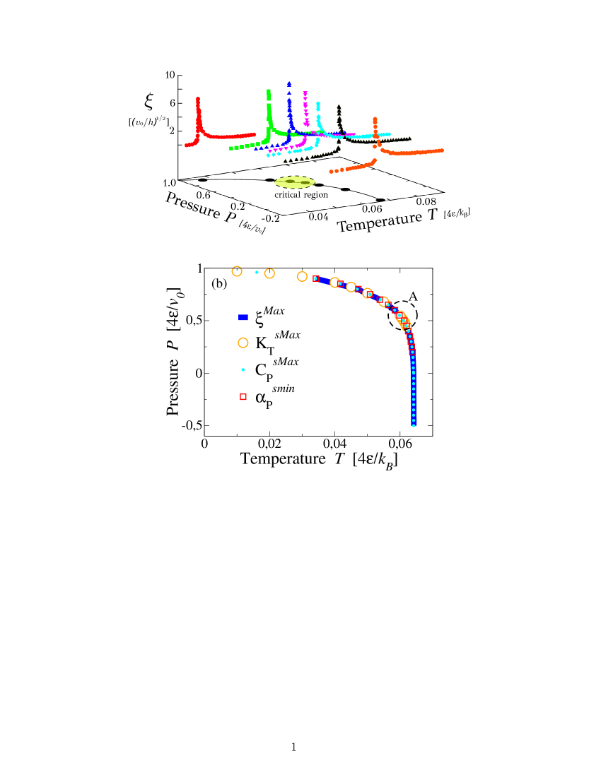
Figure 6: (a) The correlation length $\xi$ along isobars for $N=10^{4}$ water molecules has maxima that increase for $P$ approaching the critical region A. (b) The locus of $\xi$ maxima coincides with the loci of strong extrema of $K_{T}$, $C_{P}$ and $\alpha_{P}$. The Widom line is by definition the locus of $\xi$ maxima at high $T$ departing from the LLCP, that we locate within the critical region A, as discussed in the text.

At $P$ below the region $A$, we find that $\xi$ has a maximum, $\xi^{\rm Max}$, along isobars and that $\xi^{\rm Max}$ increases approaching $A$ (Fig. 6). The $\xi^{\rm Max}$ locus coincides with the locus of strong extrema of $C_{P}$, $K_{T}$ and $\alpha_{P}$ (Fig. 6b). We observe that this common locus converges to $A$ and that all the extrema increase approaching $A$. This behavior is consistent with the identification of $A$ with the critical region of the LLCP. Furthermore, we identify the common locus with the Widom line that, by definition, is the $\xi^{\rm Max}$ locus departing from the LLCP in the one-phase region xu ; FS2007 . Our calculations allow us to locate the Widom line at any $P$ down to the liquid-to-gas spinodal.

At $P$ above the region $A$, we find the continuation of the $\xi^{\rm Max}$ line, but with maxima that decrease for increasing $P$, as expected at the LL spinodal that ends in the LLCP (Fig. 6). Therefore, we identify the high-$P$ part of the $\xi^{\rm Max}$ locus with the LL spinodal. Along this line the density, the energy and the entropy of the liquid are discontinuous, as discussed in previous works FMS2003 ; Stokely2010 ; KFS2008 ; dls ; MSSSF2009 ; bb ; bbb ; Mazza .

To better locate and characterize the LLCP in $A$ we need to define the correct order parameter (o.p.) describing the LLPT. According to mixed-field finite-size scaling theory Wilding , a density-driven fluid–fluid phase transition is described by an o.p. $M\equiv\rho^{*}+su^{*}$, where $\rho*=\rho v_{0}$ represents the leading term (number density), $u\equiv E/(\epsilon N)$ is the energy density (both quantities are dimensionless) and $s$ is the mixed-field parameter. Such linear combination is necessary in order to get the rigth simmetry of the o.p. distribution $Q_{N}(M)$ at the critical point where $Q_{N}(M)\propto\tilde{p}_{d}(x)$. Here is $x\equiv B(M-M_{c})$, $B\equiv a_{M}^{-1}N^{\beta/d\nu}$, $\beta$ is the critical exponent that governs $M$, $\nu$ is the critical exponent that governs $\xi$, with $\nu$ and $\beta$ defined by the universality class, $a_{M}$ is a non-universal system-dependent parameter and $\tilde{p}_{d}$ is an universal function characteristic of the Ising fixed–point in $d$ dimensions. We adjust $B$ and $M_{c}$ so that $Q_{N}(M)$ has zero mean and unit variance.

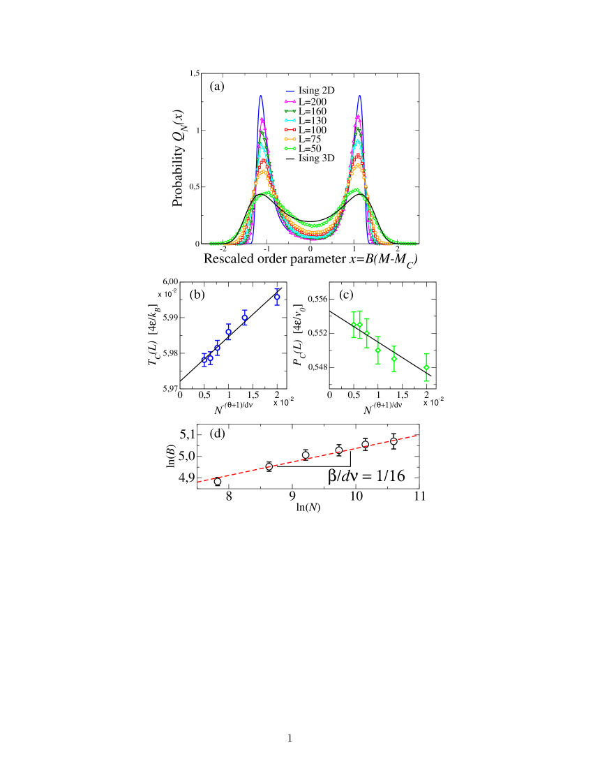
Figure 7: (a) The size-dependent probability distribution $Q_{N}$ for the rescaled o.p. $x$, calculated for $T_{c}(N)$, $P_{c}(N)$ and $B(N)$, has a symmetric shape that approaches continuously (from $N=2500$, symbols at the top at $x=0$, to $N=40000$, symbols at the bottom) the limiting form for the 2D Ising universality class (full blue line) and differs from the 3D Ising universality class case (full black line). Error bars are smaller than the symbols size. (b) The size-dependent LLCP temperature $T_{c}(N)$ and (c) pressure $P_{c}(N)$ (symbols), resulting from our best-fit of $Q_{N}$, extrapolate to $T_{c}k_{B}/(4\epsilon)\simeq 0.0597$ and $P_{c}v_{0}/(4\epsilon)\simeq 0.555$, respectively, following the expected linear behaviors (lines). (d) The normalization factor $B(N)$ (symbols) follows the power law function (dashed line) $\varpropto N^{\beta/d\nu}$. We use the $d=2$ Ising critical exponents: $\theta=2$ (correction to scaling), $\nu=1$ and $\beta=1/8$ (both defined in the text).

We combine, using the multiple histogram reweighting method hr1 described in the Methods section, a set of $3\times 10^{4}$ MC independent configurations for $\sim 300$ state points with $0.040\leq Tk_{B}/(4\epsilon)\leq 0.065$ and $0.40\leq Pv_{0}/(4\epsilon)\leq 0.75$. We verify, by tuning $s$, $T$ and $P$, that there is a point within the region $A$ where the calculated $Q_{N}(x)$ has a symmetric shape with respect to $x=0$ (Fig. 7). We find $s=0.25\pm 0.03$ for our range of $N$. The resulting critical parameters $T_{c}(N)$, $P_{c}(N)$ and the normalization factor $B(N)$ follow the expected finite-size behaviors with 2D Ising critical exponents Wilding . From the finite-size analysis we extract the asymptotic values $T_{c}k_{B}/(4\epsilon)=0.0597\pm 0.0001$ and $P_{c}v_{0}/(4\epsilon)=0.555\pm 0.002$.

The presence of a first order phase transition ending in a critical point, associated to the o.p. $M$, is confirmed by the finite size analysis of the Challa-Landau-Binder parameter cumulant of $M$

$$U_{M}\equiv 1-\dfrac{\langle M^{4}\rangle_{N}}{3\langle M^{2}\rangle^{2}_{N}}\qquad$$ (6)

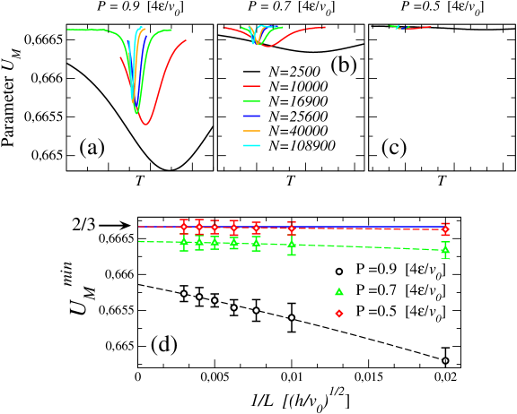
Figure 8: Challa-Landau-Binder parameter $U_{M}$ (defined in the text) of the o.p. $M$ for different system sizes, calculated for three pressures: (a) $Pv_{0}/(4\epsilon)=0.9$, (b) $Pv_{0}/(4\epsilon)=0.7$, and (c) $Pv_{0}/(4\epsilon)=0.5$ slightly below $P_{c}v_{0}/(4\epsilon)\simeq 0.555$ . The curves are calculated with the histogram reweighting method. (d) Scaling of the minima of $U_{M}$ for different $P$. The arrow points to value $2/3$ corresponding to the absence of a first-order phase transition in the thermodynamic limit. Error bars are calculated propagating the statistical error from histogram reweighting method.

where the symbol $\langle\cdotp\rangle_{N}$ refers to the thermodynamic average for a system with $N$ water molecules. $U_{M}$ quantifies the bimodality in $Q_{N}(M)$. The isobaric value of $U_{M}$ shows a minimum at the temperature where $Q_{N}(M)$ mostly deviates with respect to a symmetric distribution (Fig. 8). Minimum of $U_{M}$ converges to $2/3$ in the thermodynamic limit away from a first order phase transition, while it approaches to a value $<2/3$ where the bimodality of $Q_{N}(M)$ indicates the presence of phase coexistence.

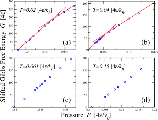
Figure 9: Gibbs free energy $G$ along isotherms, as function of $P$. Points are shifted in such a way that $G=0$ at the lowest $P$. Lines are guides for the eyes. (a) For $T=0.02(4\epsilon/k_{B})<T_{c}$ there is a discontinuity in the $P$-derivative of $G$ at $P\simeq 0.952(4\epsilon/v_{0})>P_{c}$ as expected at the LLPT, consistent with the behavior of the response functions at this state point (e.g., in Fig. 3b, 4b). (b) For $T=0.04(4\epsilon/k_{B})<T_{c}$ we observe the discontinuity in the $P$-derivative at $P\simeq 0.865(4\epsilon/v_{0})>P_{c}$, again consistent with the LLPT. The LDL has a lower chemical potential ($\mu\equiv G/N$) than the HDL, $\mu_{LDL}<\mu_{HDL}$, due to the HB energy gain in the LDL. For $T=0.061(4\epsilon/k_{B})$ (c) and for $T=0.15(4\epsilon/k_{B})$ (d), both larger than $T_{c}$, we instead do not observe any discontinuity in the $P$-derivative of $G$ by crossing the locus of $C_{P}(P)^{\rm wMax}$ and the locus of $K_{T}(T)^{\rm wMax}$, respectively, as expected in the one-phase region.

These results are consistent with the behavior of the Gibbs free energy $G$ calculated with the histogram reweighting method (Fig. 9). In particular, we calculate $G$ along isotherms, for $P$ crossing the LLPT and the loci of weak maxima in $K_{T}(T)$ and $C_{P}(P)$. We find that the behavior of $G$ for $T<T_{c}$ is consistent with the occurrence of a discontinuity in volume $V=\partial G/\partial P$, in the thermodynamic limit, with a decrease of $V$ corresponding to the transition from LDL to HDL for increasing $P$. Crossing the loci $K_{T}(T)^{\rm wMax}$ and $C_{P}(P)^{\rm wMax}$ the volume decreases with pressure without any discontinuity as expected in the one-phase region.

The distribution $Q_{N}(N)$ adjust well to the data only for large $N$. We, therefore, perform a more systematic analysis. For each $N$, we quantify the deviation of the calculated $\tilde{p}(N)$ from the expected $\tilde{p}_{2}$ for the 2D Ising. Furthermore, due to the behavior of data for small $N$ (Fig. 7a), we calculate the deviation from the 3D Ising $\tilde{p}_{3}$ Wilding . We estimate the Kullback-Leibler divergence kullback-leibler ,

$$D^{\rm KL}_{d}(N)\equiv\sum_{i=1}^{n}\ln\left(\dfrac{\tilde{p}_{d,i}}{\tilde{p}_{i}(N)}\right)\tilde{p}_{d,i}$$ (7)

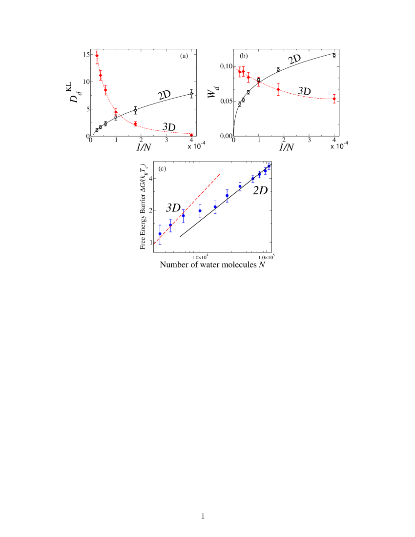
Figure 10: (a) Kullback-Leibler divergence $D^{\rm KL}_{d}(N)$ and (b) Liu et al. deviations $W_{d}$ of the calculated $\tilde{p}(N)$ from the Ising universal function $\tilde{p}_{d}$ in $d=2$ (open symbols) and $d=3$ (closed symbols), as a function of $1/N$, with $N$ water molecules, at constant $\rho\simeq\rho_{c}$. In both panels lines are power-law fits and we observe a crossover between 2D and 3D behavior at $N\simeq 10^{4}$. (c) The free-energy cost to form an interface between the two liquids coexisting at the LLCP scales as $\Delta G\propto N^{\frac{d-1}{d}}$ with $d=3$ for $N<10^{4}$ and $d=2$ for $N>10^{4}$.

of the probability distribution $\tilde{p}_{i}(N)$ of $x_{i}$ from the theoretical value $\tilde{p}_{d,i}$ of $x_{i}$ ($i=1,\dots,n$) in $d$ dimensions (Fig. 10a), and the Liu et al. deviation Liu2010 ,

$$W_{d}(N)\equiv\dfrac{1}{n}\dfrac{\sum_{i=1}^{n}\sqrt{\tilde{p}_{i}(N)}|\tilde{p}_{i}(N)-\tilde{p}_{d,i}|}{\tilde{p}_{d,{\rm peak}}-\tilde{p}_{d,x=0}}$$ (8)

with $\tilde{p}_{d,{\rm peak}}-\tilde{p}_{d,x=0}$ difference between the distribution peak and its value at $x=0$ (Fig. 10b).

We confirm $s\simeq 0.25$ for $\tilde{p}_{2}$ and find $s=0.10\pm 0.02$ for $\tilde{p}_{3}$ for our range of $N$. For both $D^{\rm KL}_{d}$ and $W_{d}$, with $d=2$ and $d=3$, we find minima at $T_{c}k_{B}/(4\epsilon)\simeq 0.06$ and $P_{c}v_{0}/(4\epsilon)\simeq 0.55$ that become stronger for increasing $N$. We find that $D^{\rm KL}_{2}$ and $W_{2}$ decrease with increasing $N$, vanishing for $N\rightarrow\infty$ (Fig. 10). Therefore, for an infinite monolayer between hydrophobic walls separated by $h\approx 0.5$ nm, the system has a LLCP that belongs to the 2D Ising universality class, as expected from our representation of the system as the 2D projection of the monolayer.

However, by increasing the confinement, i.e. reducing $N$ and $L$ at constant $\rho$, $D^{\rm KL}_{2}$ and $W_{2}$ become larger than $D^{\rm KL}_{3}$ and $W_{3}$, respectively. Therefore, the calculated $\tilde{p}(N)$ deviates from the 3D probability distribution less than from the 2D probability distribution. For $N=2500$ we find that both $D^{\rm KL}_{3}$ and $W_{3}$ have values approximately equal to those for $D^{\rm KL}_{2}$ and $W_{2}$ calculated for a system ten times larger. In particular we find $D^{\rm KL}_{3}\simeq 0$ for $N=2500$. Hence, by increasing the confinement of the monolayer at constant $\rho$, the LLCP has a behavior that approximates better the bulk LLCPnew ; llcp1 ; llcp2 ; llcp3 ; llcp4 ; llcp4_bis ; llcp5 , with a crossover between 2D and 3D-behavior occurring at $N\simeq 10^{4}$.

This dimensional crossover is confirmed by the finite-size analysis of the Gibbs free energy cost $\Delta G/(k_{B}T_{c})$ to form an interface between the two liquids in the vicinity of the LLCP, calculated as $\Delta G(N)\equiv-k_{B}T_{c}(N)[\ln\mathscr{P}_{N}^{\rm min}(\mathscr{H},V)-\ln\mathscr{P}_{N}^{\rm Max}(\mathscr{H},V)]$, where $\mathscr{P}_{N}^{\rm min}$ and $\mathscr{P}_{N}^{\rm Max}$ are the minimum and maximum values of the probability distribution $\mathscr{P}_{N}(\mathscr{H},V)$ of configurations of $N$ water molecules with energy $\mathscr{H}$ and volume $V$ at the LLCP. This quantity is expected to scale as $\Delta G\propto N^{\frac{d-1}{d}}$. We find that our data can be fitted as $N^{\frac{2}{3}}$ for small sizes and as $N^{\frac{1}{2}}$ for large sizes with a crossover around $N=10^{4}$ (Fig. 10c). Considering the value of the estimated $\rho_{c}$ in real units ($\simeq 1$g/cm³) dls , the corresponding crossover wall-size is $L\simeq 25$ nm.

Discussion

Our rationale for this dimensional crossover at fixed $h$ is that, when $L/h$ decreases toward 1, the characteristic way the critical fluctuations spread over the system, i.e. the universality class of the LLCP, resembles closely the bulk because the asymmetry among the three spatial dimensions is reduced. A similar result was found recently by Liu et al. for the gas-liquid critical point of a Lennard-Jones (LJ) system confined between walls by fixing $L$ and varying $h$ Liu2010 . However, in the case considered by Liu et al. the crossover was expected because the number of layers of particles was increased from one to several, making the system more similar to the isotropic 3D case. Here, instead, we consider always one single layer, changing the proportion $L/h$ by varying $L$. Therefore, it could be expected that the system belongs to the 2D universality class for any $L$.

Furthermore, the extrapolation of the results for the LJ liquid to our case of a monolayer with $h/r_{0}\simeq 1.7$, where $r_{0}$ is the water van der Waals diameter, would predict a dimensional crossover at $L/h\simeq 5$ Liu2010 . Here, instead, we find the crossover at $L/h\simeq 50$, i.e. one order of magnitude larger than the LJ case. We ascribe this enhancement of the crossover to (i) the presence of a cooperative HB network and (ii) the low coordination number that water has in both the monolayer and the bulk. These are the main differences between water and a LJ fluid. The cooperativity intensifies drastically the spreading of the critical fluctuations along a network, contributing to the effective dimensionality increase of the confined monolayer. Moreover, the HB network has in 3D a coordination number ($z=4$) as low as in 2D, making the first coordination shell similar in both dimensions.

Our findings are consistent with recent atomistic simulations of water nanoconfined between surfaces. zhang ; Ballenegger ; Bonthuis . Zhang et al. found that water dipolar fluctuations are enhanced in the direction parallel to the confining surfaces (hydrophobic graphene sheets) within a distance of 0.5 nm zhang . Ballenegger and Hansen found similar results for confined polar fluids, including water, within $\approx 0.5$ nm distance from the hydrophobic surface Ballenegger . Bonthuis et al. extended these results to both hydrophilic and hydrophobic confining surfaces. All these findings are consistent with our result showing the enhancement of the fluctuations of the o.p. in the direction parallel to the confining walls separated by $h\approx 0.5$ nm. Furthermore, Zhang et al. observed that the effect does not depend on the details of the water-surface interaction but stems from the very presence of interfaces zhang . This is confirmed by our study, where the water-interface interaction is purely due to excluded volume. Following the authors of Ref. zhang , this observation allows us to relate our finding for rigid surfaces to experimental results for water hydrating membranes Tielrooij , reporting new types of water dynamics in thin interfacial layers, and water nanoconfined in different types of reverse micelles Moilanen , showing that the water dynamics is governed by the presence of the interface rather than the details (e.g., the presence charged groups) of the interface.

In conclusion, we analyze the low-$T$ phase diagram of a water monolayer confined between hydrophobic parallel walls of size $L$ separated by $h\approx 0.5$ nm. We study water fluctuations associated to the thermodynamic response functions and their relations to the loci of TMD, TminD. For each response function we find two loci of extrema, one stronger at lower-$T$ and one weaker and broader at higher-$T$. These loci converge toward a critical region where the fluctuations diverge in the thermodynamic limit, defining the LLCP. We calculate the Widom line departing from the LLCP based on its definition as the locus of maxima of $\xi$ and show that it coincides with the locus of strong maxima of the response functions. We find that the LLCP belongs to the 2D Ising universality class for $L\rightarrow\infty$, with strong finite-size effects for small $L$. Surprisingly, the finite-size effects induce the LLCP universality class to converge toward the bulk case (3D Ising universality class) already for a system with a very pronounced plane asymmetry, i.e. a water monolayer of height $h\approx 0.5$ nm and $L/h\approx 50$. For normal liquid, instead, this is expected only for much smaller relative values of $L$ ($L/h\leq 5$). We rationalize this result as a consequence of two properties of the HB network: (i) its high cooperativity, that enhances the fluctuations, and (ii) its low coordination number, that makes the first coordination shell for the monolayer and the bulk similar.

Methods

The Model. We consider a monolayer formed by $N$ water molecules confined in a volume $V\equiv hL^{2}$ between two hydrophobic flat surfaces separated by a distance $h$, with $V/N\geq v_{0}\simeq 42$ ų, where $v_{0}$ is the water excluded volume. Each water molecule has four next-neighbours shr . We partition the volume into $N$ equivalent cells of height $h\backsimeq 0.5$nm and square section with size $r\equiv\sqrt{L^{2}/N}$, equal to the average distance between water molecules. By coarse-graining the molecules distance from the surfaces, we reduce our monolayer representation to a 2D system. We use periodic boundary conditions parallel to the walls to reduce finite-size effects. We simulate constant $N$, $P$, $T$, allowing $V(T,P)$ to change, with each cell $i=1,\dots,N$ having number density $\rho_{i}\equiv\rho(T,P)\equiv N/V\leq\rho_{0}\equiv 1/v_{0}$ corresponding to a mass density $\backsimeq 1$ g/cm³. To each cell we associate a variable $n_{i}=0$ ($n_{i}=1$) depending if the cell $i$ has $\rho_{i}/\rho_{0}\leq 0.5$ ($\rho_{i}/\rho_{0}>0.5$). Hence, $n_{i}$ is a discretized density field replacing the water translational degrees of freedom. The water-water interaction is given by

$$\mathscr{H}\equiv\sum_{ij}U(r_{ij})-JN_{\rm HB}-J_{\sigma}N_{\rm coop}.$$ (9)

The first term, summed over all the water molecules $i$ and $j$ at O–O distance $r_{ij}$, has $U(r)\equiv\infty$ for $r<r_{0}\equiv\sqrt{v_{0}/h}=2.9$ Å (water van der Waals diameter), $U(r)\equiv 4\epsilon[(r_{0}/r)^{12}-(r_{0}/r)^{6}]$ for $r\geq r_{0}$ with $\epsilon\equiv 5.8$ kJ/mol, and $U(r)\equiv 0$ for $r>r_{c}\equiv 25r_{0}$ (cutoff).

The second term represents the directional (covalent) component of the hydrogen bond (HB), with $J/4\epsilon\equiv 0.5$, $N_{\rm HB}\equiv\sum_{\langle ij\rangle}n_{i}n_{j}\delta_{\sigma_{ij},\sigma_{ji}}$ number of HBs, with the sum over n.n., where $\sigma_{ij}=1,\dots,q$ is the bonding index of molecule $i$ to the n.n. molecule $j$, with $\delta_{ab}=1$ if $a=b$, 0 otherwise. Each water molecule can form up to four HBs. We adopt a geometrical definition of the HB, based on the ${\widehat{\rm OOH}}$ angle and the OH—O distance. A HB breaks if ${\widehat{\rm OOH}}>30^{o}$. Hence, only $1/6$ of the entire range of values $[0,360^{\circ}]$ for the ${\widehat{\rm OOH}}$ angle is associated to a bonded state. Therefore, we choose $q=6$ to account correctly for the entropy variation due to the HB formation and breaking. Moreover, a HB breaks when the OH—O distance $>r_{\rm max}-r_{\rm OH}=3.14$ Å, where $r_{\rm OH}=0.96$ Å and $r_{\rm max}=4.1$ Å. The value of $r_{\rm max}$ is a consequence of our choice $n_{i}=0$ for $\rho_{i}/\rho_{0}\leq 0.5$, i.e. $r_{i}^{2}/2\geq r_{0}^{2}$, implying that $n_{i}n_{j}=0$ when $r_{ij}\geq r_{0}\sqrt{2}=4.10$ Å $\equiv r_{\rm max}$.

The third term of the Eq.(9) accounts for the HB cooperativity due to the quantum many-body interaction Hernandez , with $J_{\sigma}/4\epsilon\equiv 0.05$ and $N_{\rm coop}\equiv\sum_{i}n_{i}\sum_{(l,k)_{i}}\delta_{\sigma_{ik},\sigma_{il}}$, where $(l,k)_{i}$ indicates each of the six different pairs of the four indices $\sigma_{ij}$ of a molecule $i$. The value $J_{\sigma}\ll J$ is chosen in such a way to guarantee an asymmetry between the two components of the HB interaction. To the cooperative term is due the O–O–O correlation that locally leads the molecules toward an ordered configuration. In bulk water this term would lead to a tetrahedral structure at low $P$ up to the second shell, as observed in the experiments SoperRicci2000 . An increase of $T$ or $P$ partially disrupts the HB network and induces a more compact local structure, with smaller average volume per molecule. Therefore, for each HB we include an enthalpy increase $Pv_{\rm HB}$, where $v_{\rm HB}/v_{0}=0.5$ is the average volume increase between high-$\rho$ ices VI and VIII and low-$\rho$ (tetrahedral) ice Ih. Hence, the total volume is $V\equiv V_{0}+N_{\rm HB}v_{\rm HB}$, where $V_{0}\geq Nv_{0}$ is a stochastic continuous variable changing with Monte Carlo (MC) acceptance rule MSSSF2009 . Because the HBs do not affect the n.n. distance SoperRicci2000 , we ignore their negligible effect on the $U(r)$ term. Finally, we model the water-wall interaction by excluded volume.

The Observables. The LLCP is identified by the mixed-field order parameter $M$ and not by the magnetization of the Potts variables $\sigma_{i,j}$ as in normal Potts model. $M$ is related to the configuration of the system by the relation

$$M\equiv\dfrac{N}{Nv+\sum_{\langle ij\rangle}n_{i}n_{j}\delta_{\sigma_{ij},\sigma_{ji}}}+s\left(U(r)-J\sum_{\langle ij\rangle}n_{i}n_{j}\delta_{\sigma_{ij},\sigma_{ji}}-J_{\sigma}\sum_{i}n_{i}\sum_{(l,k)_{i}}\delta_{\sigma_{ik},\sigma_{il}}\right)$$ (10)

where $v\equiv V_{0}/N$ and $s$ is the mixed-field parameter. $M$ is therefore a linear combination of the density and energy.

Thermodynamic response functions are calculated from

$$K_{T}\equiv-\frac{1}{\langle V\rangle}\left(\frac{\partial\langle V\rangle}{\partial P}\right)_{T}=\frac{\langle\Delta V^{2}\rangle}{k_{B}TV}$$ (11)

and

$$C_{P}\equiv\left(\frac{\partial\langle H\rangle}{\partial T}\right)_{P}=\frac{\langle\Delta H^{2}\rangle}{k_{B}T}$$ (12)

as long as the volume and energy distributions are not clearly bimodal, i.e. excluding the values of $T$ and $P$ where the phase coexistence is observed, based on the definition of $M$. Here $\Delta O\equiv O-\langle O\rangle$, for $O=V,H$ and, $H$ is the enthalpy of the system.

The Monte Carlo Method. The system is equilibrated via Monte Carlo simulation with Wolff algorithm MSSSF2009 , following an annealing procedure: starting with random initial condition at high $T$, the temperature is slowly decreased and the system is re-equilibrated and sampled with $10^{4}\div 10^{5}$ independent configurations for each state point. The thermodynamic equilibrium is checked probing that the fluctuation-dissipation relations, Eq. (11) and (12), hold within the error bar.

The Histogram Reweighting Method. The probability $Q_{N}(M)$ is calculated in a continuous range of $T$ and $P$ across the $\xi^{\rm Max}$ line. We consider an initial set of $m\in[10:20]$ independent simulations within a temperature range $\Delta Tk_{B}/(4\epsilon)\sim 10^{-4}$ and a pressure range $\Delta Pv_{0}/(4\epsilon)\sim 10^{-3}$. For each simulation $i=1,...,m$ we calculate the histograms $h_{i}(u,\rho)$ in the energy density–density plane. The histograms $h_{i}(u,\rho)$ provide an estimate of the equilibrium probability distribution for $u$ and $\rho$; this estimate becomes correct in the thermodynamic limit. For the $NPT$ ensemble, the new histogram $h(u,\rho,P^{\prime},\beta^{\prime})$ for new values of $\beta^{\prime}=1/k_{B}T^{\prime}$ and $P^{\prime}$ close the simulated ones, is given by the relation hr1

$$h(u,\rho,P^{\prime},\beta^{\prime})=\dfrac{\sum_{i=1}^{m}h_{i}(u,\rho)e^{-\beta^{\prime}(u+P^{\prime}/\rho)N}}{\sum_{i=1}^{m}N_{i}e^{-\beta_{i}(u+P_{i}/\rho)N-C_{i}}}$$ (13)

where $N_{i}$ is the number of independent configurations of the run $i$. The constants $C_{i}$, related to the Gibbs free energy value at $T_{i}$ and $P_{i}$, are self-consistently calculated from the equation hr1

$$e^{C_{i}}=\sum_{u}\sum_{\rho}h(u,\rho,P_{i},\beta_{i})\simeq Z(P_{i},\beta_{i})\qquad\Rightarrow\qquad C_{i}=-G(P_{i},\beta_{i})/k_{B}T\text{ }.$$ (14)

We choose as initial set of parameters $C_{i}=0$. The parameters $C_{i}$ are recursively calculated by means of Eq. (13) and (14) until the difference between the values at iteration $k$ and $k+1$ is less then the desired numerical resolution ($10^{-3}$ in our calculations). Once the new histogram is calculated, $Q_{N}(M)$ at $T_{i}$ and $P_{i}$ is calculated integrating $h(u,\rho,P_{i},\beta_{i})$ along a direction perpendicular to the line $\rho+su$.

Thermodynamic relations. We report here the calculations for the thermodynamic relations in Eq. (1), (2), (3) and (4) sf . To verify the relation (4) we calculate the derivative of $K_{T}$ along isobars

$$\begin{array}[]{ll}\left(\dfrac{\partial K_{T}}{\partial T}\right)_{P}=\dfrac{\partial}{\partial T}\left(-\dfrac{1}{V}\left(\dfrac{\partial V}{\partial P}\right)_{T}\right)_{P}=\dfrac{1}{V^{2}}\left(\dfrac{\partial V}{\partial T}\right)_{P}\left(\dfrac{\partial V}{\partial P}\right)_{T}-\dfrac{1}{V}\dfrac{\partial^{2}V}{\partial P\partial T}=-\alpha_{P}K_{T}-\dfrac{1}{V}\dfrac{\partial^{2}V}{\partial P\partial T}\end{array}$$ (15)

and the derivative of $\alpha_{P}$ along isotherms

$$\begin{array}[]{ll}\left(\dfrac{\partial\alpha_{P}}{\partial P}\right)_{T}&=\dfrac{\partial}{\partial P}\left(\dfrac{1}{V}\left(\dfrac{\partial V}{\partial T}\right)_{P}\right)_{T}=-\dfrac{1}{V^{2}}\left(\dfrac{\partial V}{\partial P}\right)_{T}\left(\dfrac{\partial V}{\partial T}\right)_{P}+\dfrac{1}{V}\dfrac{\partial^{2}V}{\partial T\partial P}=\\ \\ &=\alpha_{P}K_{T}+\dfrac{1}{V}\dfrac{\partial^{2}V}{\partial P\partial T}=-\left(\dfrac{\partial K_{T}}{\partial T}\right)_{P}\end{array}$$ (16)

Following sf ; rebelo the line of extrema in density (TMD and TminD lines) is characterized by $\alpha_{P}=0$, hence, $d\alpha_{P}=0$ along the TMD line. Therefore,

$$\begin{array}[]{ll}0=d\alpha_{P}\equiv\left(\dfrac{\partial\alpha_{P}}{\partial T}\right)_{P,~{}\rm ED}dT+\left(\dfrac{\partial\alpha_{P}}{\partial P}\right)_{T,~{}\rm ED}dP=\left(\dfrac{1}{V}\dfrac{\partial^{2}V}{\partial T^{2}}\right)_{P,~{}\rm ED}dT+\left(\dfrac{1}{V}\dfrac{\partial^{2}V}{\partial P\partial T}\right)_{\rm ED}dP\end{array}$$ (17)

where the index “ED” denotes that the derivatives are taken along the locus of extrema in density. So, the slope $\partial P/\partial T$ of TMD is given by

$$\left(\frac{\partial P}{\partial T}\right)_{\rm TMD}=-\dfrac{\left(\dfrac{\partial^{2}V}{\partial T^{2}}\right)_{P,~{}\rm TMD}}{\left(\dfrac{\partial^{2}V}{\partial P\partial T}\right)_{\rm TMD}}$$ (18)

from which, using Eq. (15) with $\alpha_{P}=0$, we get Eq. (1). The Eq. (18) holds as long as both $(\partial\alpha_{P}/\partial P)_{T}$ and $(\partial\alpha_{P}/\partial T)_{P}$ do not vanish contemporary, as it occurs along the Widom line, where the loci of strong minima of $\alpha_{P}$ overlap. For this reason the intersection between the Widom line and TminD line does not imply any change in the slope $(\partial P/\partial T)_{\rm TminD}$.

To calculate Eq. (2) we start from $C_{P}$ and $\alpha_{P}$ written in terms of Gibbs free energy

$$\frac{C_{P}}{T}=-\frac{\partial^{2}G}{\partial T^{2}}\qquad,\qquad V\alpha_{P}=\frac{\partial^{2}G}{\partial P\partial T}$$ (19)

from which results

$$\begin{array}[]{ll}\dfrac{\partial}{\partial P}\left(\dfrac{C_{P}}{T}\right)_{T}=\dfrac{1}{T}\left(\dfrac{\partial C_{P}}{\partial P}\right)_{T}=-\left[\dfrac{\partial}{\partial T}\left(V\alpha_{P}\right)\right]_{P}=-\left(\dfrac{\partial V}{\partial T}\right)_{P}\alpha_{P}-V\left(\dfrac{\partial\alpha_{P}}{\partial T}\right)_{P}=-\left(\dfrac{\partial^{2}V}{\partial T^{2}}\right)_{P}\qquad,\end{array}$$ (20)

$$\left(\dfrac{\partial C_{P}}{\partial P}\right)_{T}=-T\left(\dfrac{\partial^{2}V}{\partial T^{2}}\right)_{P}\qquad.$$ (21)

Substituting in Eq. (18) we get the Eq. (2) at the TMD. Moreover, because of $\alpha_{P}=0$ at the TMD line, from the last equivalence of Eq. (20) we get

$$\left(\dfrac{\partial\alpha_{P}}{\partial T}\right)_{P,~{}\rm TMD}=\dfrac{1}{V}\left(\dfrac{\partial^{2}V}{\partial T^{2}}\right)_{P,~{}\rm TMD}$$ (22)

from which, using Eq. (18), we get the Eq. (3).

REFERENCES

ACKNOWLEDGEMENTS

We acknowledge the support of Spanish MEC grant FIS2012-31025 and the EU FP7 grant NMP4-SL-2011-266737.

AUTHOR CONTRIBUTION STATEMENT

V. B. and G. F. designed the research. V. B. made the simulations. G. F. supervised the work. Both authors analyzed the data, prepared the figures, wrote the text and reviewed the manuscript.

ADDITIONAL INFORMATION

The authors declare no competing financial interests.

REFERENCES

- (1) Paul, D. R. Creating New Types of Carbon-Based Membranes., Science 335, 413 (2012).
- (2) Zhang, Y. et al., Density hysteresis of heavy water confined in a nanoporous silica matrix., Proc. Natl. Acad. Sci. USA 108, 12206 (2011).
- (3) Soper, A. Density minimum in supercooled confined water., Proc. Natl. Acad. Sci. USA 47, E1192 (2011).
- (4) Whitby, M. & Quirke, N. Fluid flow in carbon nanotubes and nanopipes., Nat. Nanotechnol 2, 87 (2007).
- (5) Han, S., Choi, M. Y., Kumar, P. & Stanley, H. E. Phase transitions in confined water nanofilms., Nat. Phys. 6, 685-689 (2010).
- (6) Faraudo J. & Bresme, F. Anomalous Dielectric Behavior of Water in Ionic Newton Black Films., Phys. Rev. Lett. 92, 236102 (2004).
- (7) Zangi, R., Mark, A. E. Monolayer Ice., Phys. Rev. Lett. 91, 025502 (2003).
- (8) Mishima, O. & Stanley, H. E. The relationship between liquid, supercooled and glassy water., Nature 396, 329 (1998).
- (9) Nilsson, A. et al. Resonant inelastic X-ray scattering of liquid water., J. Electron. Spectrosc. 188, 84–10 (2013).
- (10) Taschin, A., Bartolini, P., Eramo, R., Righini, R., & Torre, R. Evidence of two distinct local structures of water from ambient to supercooled conditions., Nature Comm. 4, 2401 (2013).
- (11) Poole, P. H., Sciortino, F., Essmann, U. & Stanley, H. E. Phase-Behavior Of Metastable Water., Nature 360, 324 (1992).
- (12) Katayama, Y. et al. A first-order liquid-liquid phase transition in phosphorus., Nature 403, 170 (2000).
- (13) Katayama, Y. et al. Macroscopic Separation of Dense Fluid Phase and Liquid Phase of Phosphorus., Science 306, 848 (2004).
- (14) Monaco, G., Falconi, S., Crichton, W. A. & Mezouar, M. Nature of the First-Order Phase Transition in Fluid Phosphorus at High Temperature and Pressure., Phys. Rev. Lett. 90, 255701 (2003).
- (15) Tanaka, H., Kurita, R. & Mataki, H. Liquid-Liquid Transition in the Molecular Liquid Triphenyl Phosphite., Phys. Rev. Lett. 92, 025701 (2004).
- (16) Kurita, R. & Tanaka, H. Critical-Like Phenomena Associated with Liquid-Liquid Transition in a Molecular Liquid., Science 306, 845 (2004).
- (17) Greaves, G. N. et al. Detection of First-Order Liquid/Liquid Phase Transitions in Yttrium Oxide-Aluminum Oxide Melts., Science 322, 566 (2008).
- (18) Murata, K.-i. & Tanaka, H. Liquid–liquid transition without macroscopic phase separation in a water–glycerol mixture., Nature Mater. 11, 436 (2012).
- (19) Tanaka, H. Bond orientational order in liquids: Towards a unified description of water-like anomalies, liquid-liquid transition, glass transition, and crystallization - Bond orientational order in liquids., Eur. Phys. J. E 35, 113 (2012).
- (20) Murata, K-i. & Tanaka, H. General nature of liquid–liquid transition in aqueous organic solutions., Nature Comm. 4, 2844 (2013).
- (21) Machon, D., Meersman, F., Wilding, M.C., Wilson, M. & McMillan, P. F. Pressure-induced amorphization and polyamorphism: Inorganic and biochemical systems., Prog. Mater. Sci. 61, 216-282 (2014).
- (22) Bertrand, C. E. & Anisimov, M. A. Peculiar Thermodynamics of the Second Critical Point in Supercooled Water., J. Phys. Chem. B 115, 14099 (2011).
- (23) Holten, V. & Anisimov, M. A. Entropy-driven liquid-liquid separation in supercooled water., Sci. Rep. 2, 713 (2012).
- (24) Nilsson, A., Huang, C., Pettersson, L. G. M. Fluctuations in ambient water., J. Mol. Liq. 176, 2–16 (2012).
- (25) Tanaka, H. A self-consistent phase diagram for supercooled water., Nature 380, 328 (1996).
- (26) Abascal, J. L. F. & Vega, C. Widom line and the liquid-liquid critical point for the TIP4P/2005 water model., J. Chem. Phys. 133, 234502 (2010).
- (27) Sciortino, F., Saika-Voivod, I. & Poole, P. H. Study of the ST2 model of water close to the liquid-liquid critical point., Phys. Chem. Chem. Phys., 13, 19759 (2011).
- (28) Kesselring, T., Franzese, G., Buldyrev, S., Herrmann, H. & Stanley, H. E. Nanoscale Dynamics of Phase Flipping in Water near its Hypothesized Liquid-Liquid Critical Point., Sci. Rep. 2, 474 (2012).
- (29) Kesselring, T. A. et al. Finite-size scaling investigation of the liquid-liquid critical point in ST2 water and its stability with respect to crystallization., J. Chem. Phys. 138 , 244506 (2013)
- (30) Poole, P. H., Bowles, R. K., Saika-Voivod, I. & Sciortino, F. Free energy surface of ST2 water near the liquid-liquid phase transition., J. Chem. Phys. 138, 034505 (2013).
- (31) Franzese, G., Marques, M. I. & Stanley, H. E. Intramolecular coupling as a mechanism for a liquid-liquid phase transition., Phys. Rev. E 67, 011103 (2003).
- (32) Franzese, G., Malescio, G., Skibinsky, A., Buldyrev, S. V. & Stanley, H. E. Generic mechanism for generating a liquid-liquid phase transition., Nature 409, 692 (2001).
- (33) Sastry, S. & Angell, C. A. Liquid-liquid phase transition in supercooled silicon., Nature Mater. 2, 739 (2003).
- (34) Scandolo, S. Liquid–liquid phase transition in compressed hydrogen from first-principles simulations., Proc. Natl. Acad. Sci. USA 100 3051 (2003).
- (35) Ganesh, P. & Widom, M. Liquid-Liquid Transition in Supercooled Silicon Determined by First-Principles Simulation., Phys. Rev. Lett. 102, 075701 (2009).
- (36) Vilaseca, P. & Franzese, G. Isotropic soft-core potentials with two characteristic length scales and anomalous behaviour., J. Non-Cryst. Sol. 357, 419 (2011).
- (37) Gallo, P. & Sciortino, F. Ising Universality Class for the Liquid-Liquid Critical Point of a One Component Fluid: A Finite-Size Scaling Test., Phys. Rev. Lett. 109, 77801 (2012).
- (38) Liu, Y., Palmer, J. C., Panagiotopoulos, A. Z. & Debenedetti, P. G. Liquid-liquid transition in ST2 water., J. Chem. Phys. 137, 214505 (2012).
- (39) Sastry, S., Debenedetti, P. G., Sciortino, F. & Stanley, H. E. Singularity-free interpretation of the thermodynamics of supercooled water., Phys. Rev. E 53, 6144 (1996).
- (40) Stokely, K., Mazza, M. G., Stanley, H. E., Franzese, G. Effect of hydrogen bond cooperativity on the behavior of water., Proc. Natl. Acad. Sci. USA 107, 1301 (2010).
- (41) Limmer, D. T. & Chandler, D. The putative liquid–liquid transition is a liquid–solid transition in atomistic models of water., J. Chem. Phys. 135, 134503 (2011).
- (42) Palmer, J. C., Car, R. & Debenedetti, P. G. The Liquid-Liquid Transition in Supercooled ST2 Water: a Comparison Between Umbrella Sampling and Well-Tempered Metadynamics., Faraday Discuss. 167, (2013).
- (43) Gallo, P. & Rovere, M. Special section on water at interfaces, J. Phys.: Cond. Matt. 22, 280301 (2010).
- (44) Strekalova, E. G., Mazza, M. G., Stanley, H. E. & Franzese, G. Large Decrease of Fluctuations for Supercooled Water in Hydrophobic Nanoconfinement. Phys. Rev. Lett. 106, 145701 (2011).
- (45) de los Santos, F. & Franzese, G. Understanding Diffusion and Density Anomaly in a Coarse-Grained Model for Water Confined between Hydrophobic Walls. J. Phys. Chem. B 115, 14311 (2011).
- (46) Mazza, M. G., Stokely, K., Strekalova, E. G., Stanley, H. E. & Franzese, G. Cluster Monte Carlo and numerical mean field analysis for the water liquid-liquid phase transition. Comp. Phys. Comm. 180, 497 (2009).
- (47) Franzese, G., Bianco, V. & Iskrov, S. Water at Interface with Proteins. Food Biophys. 6, 186 (2011).
- (48) Bianco, V., Iskrov, S. & Franzese, G. Understanding the role of hydrogen bonds in water dynamics and protein stability. J. Biol. Phys. 38, 27 (2012).
- (49) Mazza, M. G., Stokely, K., Pagnotta, S. E., Bruni, F., Stanley, H. E. & Franzese, G. More than one dynamic crossover in protein hydration water. Proc. Natl. Acad. Sci. USA 108, 19873 (2011).
- (50) Franzese, G., Bianco, V. Water at Biological and Inorganic Interfaces. Food Biophys. 8, 153 (2013).
- (51) Mallamace, F., Branca, C., Broccio, M., Corsaro, C., Mou, C.-Y. & Chen, S.-H. The anomalous behavior of the density of water in the range 30 K T 373 K. Proc. Natl. Acad. Sci. USA 104, 18387 (2007).
- (52) Poole, P. H., Saika-Voivod, S. & Sciortino, F. Density minimum and liquid-liquid phase transition. J. Phys.: Cond. Matt. 17, L431 (2005).
- (53) Xu, L. et al. Relation between the Widom line and the dynamic crossover in systems with a liquid-liquid phase transition. Proc. Natl. Acad. Sci. USA 46, 16558 (2005).
- (54) Franzese, G. Stanley, H. E. The Widom line of supercooled water., J. Phys.: Cond. Matt. 20, 205126 (2007).
- (55) Wilding, N. B. & Binder, K. Finite-size scaling for near-critical continuum fluids at constant pressure., Phys. A 1, 439 (1996).
- (56) Panagiotopoulos, A. Z. Monte Carlo methods for phase equilibria of fluids., J. Phys.: Cond. Matt. 12, R25 (2000) for a review.
- (57) Franzese, G. Coniglio, A. Phase transitions in the Potts spin-glass model., Phys. Rev. E 58, 2753 (1998).
- (58) Kullback, S. & Leibler, R. A. On Information and Sufficiency., Ann. Math. Statist. 22, 79-86 (1951).
- (59) Liu, Y., Panagiotopoulos, A. Z. & Debenedetti, P. G. Finite-size scaling study of the vapor-liquid critical properties of confined fluids: Crossover from three dimensions to two dimensions. J. Chem. Phys. 132, 144107 (2010).
- (60) Zhang, C., Gygi, F. & Galli, G. Strongly Anisotropic Dielectric Relaxation of Water at the Nanoscale., J. Phys. Chem. Lett. 4, 2477–2481 (2013).
- (61) Ballenegger, V. & Hansen, J.-P. Dielectric permittivity profiles of confined polar fluids., J. Chem. Phys. 122, 114711 (2011).
- (62) Bonthuis, D. J., Gekle, S. & Netz, R. R. Dielectric Profile of Interfacial Water and its Effect on Double-Layer Capacitance., Phys. Rev. Lett. 107, 166102 (2011).
- (63) Tielrooij, K. J., Paparo, D., Piatkowski, L., Bakker, H. J. & Bonn, M. Dielectric Relaxation Dynamics of Water in Model Membranes Probed by Terahertz Spectroscopy., Biophys. J. 97, 2484–2492 (2009).
- (64) Moilanen, D. E., Levinger, N. E., Spry, D. B. & Fayer, M. D. Confinement or the Nature of the Interface? Dynamics of Nanoscopic Water., J. Am. Chem. Soc. 129, 14311–14318 (2007).
- (65) Hernández de la Peña, L. & Kusalik, P. G. Temperature Dependence of Quantum Effects in Liquid Water., J. Am. Chem. Soc. 127, 5246 (2005).
- (66) Soper, A. K. & Ricci, M. A. Structures of high-density and low-density water., Phys. Rev. Lett. 84, 2881 (2000).
- (67) Rebelo, L. P. N., Debenedetti, P. G. & Sastry, S. Singularity-free interpretation of the thermodynamics of supercooled water. II. Thermal and volumetric behavior., J. Chem. Phys. 109, 626 (1998).