Move-by-move dynamics of the advantage in chess matches reveals population-level learning of the game

Abstract

The complexity of chess matches has attracted broad interest since its invention. This complexity and the availability of large number of recorded matches make chess an ideal model systems for the study of population-level learning of a complex system. We systematically investigate the move-by-move dynamics of the white player’s advantage from over seventy thousand high level chess matches spanning over 150 years. We find that the average advantage of the white player is positive and that it has been increasing over time. Currently, the average advantage of the white player is $\sim$0.17 pawns but it is exponentially approaching a value of 0.23 pawns with a characteristic time scale of 67 years. We also study the diffusion of the move dependence of the white player’s advantage and find that it is non-Gaussian, has long-ranged anti-correlations and that after an initial period with no diffusion it becomes super-diffusive. We find that the duration of the non-diffusive period, corresponding to the opening stage of a match, is increasing in length and exponentially approaching a value of 15.6 moves with a characteristic time scale of 130 years. We interpret these two trends as a resulting from learning of the features of the game. Additionally, we find that the exponent $\alpha$ characterizing the super-diffusive regime is increasing toward a value of 1.9, close to the ballistic regime. We suggest that this trend is due to the increased broadening of the range of abilities of chess players participating in major tournaments.

Introduction

The study of biological and social complex systems has been the focus of intense interest for at least three decades Amaral . Elections Fortunato , popularity Ratkiewicz , population growth Rozenfeld , collective motion of birds Bialek and bacteria Peruani are just some examples of complex systems that physicists have tackled in these pages. An aspect rarely studied due to the lack of enough data over a long enough period is the manner in which agents learn the best strategies to deal with the complexity of the system. For example, as the number of scientific publication increases, researchers must learn how to choose which papers to read in depth Stringer ; while in earlier times word-of-mouth or listening to a colleague’s talk were reliable strategies, nowadays the journal in which the study was published or the number of citations have become, in spite of their many caveats, indicators that seem to be gaining in popularity.

In order to understand how population-level learning occurs in the “real-word,” we study it here in a model system. Chess is a board game that has fascinated humans ever since its invention in sixth-century India OBrien . Chess is an extraordinary complex game with $10^{43}$ legal positions and $10^{120}$ distinct matches, as roughly estimated by Shannon Shannon . Recently, Blasius and Tönjes Blasius have showed that scale-free distributions naturally emerge in the branching process in the game tree of the first game moves in chess. Remarkably, this breadth of possibilities emerges from a small set of well-defined rules. This marriage of simple rules and complex outcomes has made chess an excellent test bed for studying cognitive processes such as learning Gobet ; Saarilouma and also for testing artificial intelligence algorithms such as evolutionary algorithms Fogel .

The very best chess players can foresee the development of a match 10–15 moves into the future, thus making appropriate decisions based on his/her expectations of what his opponent will do. Even though super computers can execute many more calculations and hold much more information in a quickly accessible mode, it was not until heuristic rules were developed to prune the set of possibilities that computers became able to consistently beat human players. Nowadays, even mobile chess programs such as Pocket Fritz™ (http://chessbase-shop.com/en/products/pocket_fritz_4) have a Elo rating Elo of $2938$ which is higher than the current best chess player (Magnus Carlsen with a Elo rating of 2835 — http://fide.com).

The ability of many chess engines to accurately evaluate the strength of a position enables us to numerically evaluate the move-by-move white player advantage $A(m)$ and to determine the evolution of the advantage during the course of a chess match. In this way, we can probe the patterns of the game to a degree not before possible and can attempt to uncover population-level learning in the historical evolution of chess match dynamics. Here, we focus on the dynamical aspects of the game by studying the move-by-move dynamics of the white player’s advantage $A(m)$ from over seventy thousand high level chess matches.

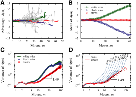
We have accessed the portable game notation (PGN) files of 73,444 high level chess matches made free available by PGN Mentor™ (http://www.pgnmentor.com). These data span the last two centuries of the chess history and cover the most important worldwide chess tournaments, including the World Championships, Candidate Tournaments, and the Linares Tournaments (see supplementary Table 1). White won $33\%$ of these matches, black won $24\%$ and $43\%$ ended up with in a draw. For each of these 73,444 matches, we estimated $A(m)$ using the Crafty™ Crafty chess engine which has an Elo rating of 2950 (see Methods Section A). The white player advantage $A(m)$ takes into account the differences in the number and the value of pieces, as well as the advantage related to the placement of pieces. It is usually measured in units of pawns, meaning that in the absence of other factors, it varies by one unit when a pawn (the pieces with lowest value) is captured. A positive value indicates that the white player has the advantage and a negative one indicates that the black player has the advantage. Figure 1A illustrates the move dependence of $A$ for 50 matches selected at random from the data base. Intriguingly, $A(m)$ visually resembles the “erratic” movement of diffusive particles.

Figure 1: Diffusive dynamics of white player’s advantage. (A) Evolution of the advantage $A(m)$ for $50$ matches selected at random. We highlight the trajectories from three World Chess Championship matches: the $6^{\text{th}}$ match between Anand (playing white) and Kramnik in 2008 (green line), the $2^{\text{nd}}$ match between Karpov (playing white) and Kasparov in 1985 (red line), and the $1^{\text{st}}$ match between Spassky (playing white) and Petrosian in 1969 (blue line). (B) Mean value of the advantage as a function of move number for matches ending in draws (squares), white wins (circles) and black wins (triangles). Note the systematically alternating values and the initial positive values of these means for all outcomes. For white wins, the mean advantage increases with $m$, while for black wins it decreases. For draws, the mean advantage is approximately a positive constant. We estimated the advantage of playing white to be $0.14\pm 0.01$ and horizontal dashed line represents this value. (C) Variance of the advantage as a function of move number for matches ending in draws (squares) and white wins (circles) and black wins (triangles). Note the very similar profile of the variance for white and black wins. Note also that there is practically no diffusion for the initial $7-10$ moves, corresponding to the opening period, a very well studied stage of the game. After the opening stage, the trajectories exhibit a faster than diffusive spreading. For draws, we find this second regime ($10<m<100$) to be superdiffusive and characterized by an exponent $\alpha=1.49\pm 0.01$, as shown by the dashed line. For wins, the variance presents a more complex behavior. For $10\lesssim m\lesssim 40$ the variance increases faster than ballistic (hyper-diffusion), but for later stages it displays a behavior similar to that found for draws. (D) Variance of advantage evaluated after grouping the matches by length and outcome. For draws (continuous lines), the different match lengths do not change the power-law dependence of the variance. For wins (dashed lines), the variance systematically approaches the profile obtained for draws as the matches becomes longer. We further note the existence of a very fast diffusive regime for the latest moves of each grouping.

Results

We first determined how the mean value of the advantage depends on the move number $m$ across all matches with the same outcome (Fig. 1B). We observed an oscillatory behavior around a positive value with a period of $1$ move for both match outcomes. This oscillatory behavior reflects the natural progression of a match, that is, the fact that the players alternate moves. Not surprisingly, for matches ending in a draw the average oscillates around an almost stable value, while for white wins it increases systematically and for black wins it decreases systematically.

Figure 1B suggests an answer to an historical debate among chess players: Does playing white yield an advantage? Some players and theorists argue that because the white player starts the game, white has the “initiative,” and that black must endeavor to equalize the situation. Others argue that playing black is advantageous because white has to reveal the first move. Chess experts usually mention that white wins more matches as evidence of this advantage. However, the winning percentage does not indicate the magnitude of this advantage. In our analysis, we not only confirm the existence of an advantage in playing white, but also estimate its value as $0.14\pm 0.01$ by averaging the values of the mean for matches ending in draws.

We next investigated the diffusive behavior by evaluating the dependence of the variance of $A$ on the move number $m$ (Fig. 1C). After grouping the matches by match outcome, we observed for all outcomes that there is practically no diffusion during the initial moves. These moves correspond to the opening period of the match, a stage very well studied and for which there are recognized sequences of moves that result in balanced positions. After this initial stage, the variance exhibits an anomalous diffusive spreading. For matches ending in a draw, we found a super-diffusive regime ($10<m<100$) that is described by a power law with an exponent $\alpha=1.49\pm 0.01$. We note the very similar profile of the variance of matches ending in white or black wins.

Matches ending in a win display an hyper-diffusive regime ($\alpha>2$) — a signature of nonlinearity and out-of-equilibrium systems Siegle . In fact, the behavior for matches ending in wins is quite complex and dependent on the match length (Fig. 1D). While grouping the matches by length does not change the variance profile of draws, for wins it reveals a very interesting pattern: As the match length increases the variance profile become similar to the profile of draws, with the only differences occurring in the last moves. This result thus suggests that the behavior of the advantage of matches ending in a win is very similar to a draw. The main difference occurs in last few moves where an avalanche-like effect makes the advantage undergo large fluctuations.

Historical Trends

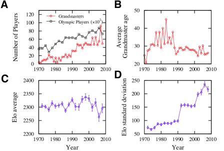
Chess rules have been stable since the 19th century. This stability increased the game popularity (Fig. 2A) and enabled players to work toward improving their skill. A consequence of these efforts is the increasing number of Grandmasters — the highest title that a player can attain — and the decreasing average player’s age for receiving this honor (Figs. 2A and 2B). Intriguingly, the average player’s fitness (measured as the Elo rating Elo ) in Olympic tournaments has remained almost constant, while the standard deviation of the player’s fitness has increased fivefold (Figs. 2C and 2D). These historical trends prompt the question of whether there has been a change in the diffusive behavior of the match dynamics over the last 150 years.

Figure 2: Historical changes in chess player demographics. (A) Number of new Chess Grandmaster awarded annually by the world chess organization (http://fide.com) and the number of players who have participated in the Chess Olympiad (http://www.olimpbase.org) since 1970. Note the increasing trends in these quantities. (B) Average players’ age when receiving the Grandmaster title. (C) Average Elo rating and (D) standard deviation of the of Elo rating of players who have participated in the Chess Olympiad. Note the nearly constant value of the average, while the standard deviation has increased dramatically.

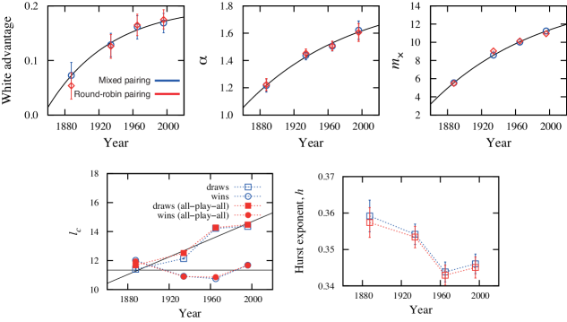
To answer this question, we investigated the evolution of the profile of the mean advantage for different periods (Fig. 3A). For easier visualization, we applied a moving averaging with window size two to the mean values of $A(m)$. The horizontal lines show the average values of the means for $20<m<40$ and the shaded areas are $95\%$ confidence intervals obtained via bootstrapping. The average values are significantly different, showing that the baseline white player advantage has increased over the last 150 years. We found that this increase is well described by an exponential approach with a characteristic time of $67.0\pm 0.1$ years to an asymptotic value of $0.23\pm 0.01$ pawns (Fig. 3C). Our results thus suggest that chess players are learning how to maximize the advantage of playing white and that this advantage is bounded.

Figure 3: Historical trends in the dynamics of highest level chess matches. (A) Mean value of the advantage of matches ending a draw for three time periods. These curves were smoothed by using moving averaging over windows of size 2. The horizontal lines are the averaged values of the mean for $20<m<40$ and the shaded regions are $95\%$ confidence intervals for these averaged values. (B) Variance of the advantage of matches ending a draw for three time periods. The shaded regions are $95\%$ confidence intervals for the variance and the colored dashed lines indicate power law fits to each data set. The horizontal dashed line represents the average variance for the most recent data set and for $1<m<10$. Note the systematic increase of $\alpha$ and of the number of moves in the opening. The symbols on this line indicate the values of $m_{\times}$, the number of moves at which the diffusion of the advantage changes behavior. The rightmost symbol represent the extrapolated maximum value $m_{\times}=15.6\pm 0.6$. (C) Time evolution of the white player advantage for matches ending in draws. The solid line represents an exponential approach to an asymptotic value. The estimated plateau value is $0.23\pm 0.01$ pawns and the characteristic time is $67.0\pm 0.1$ years. Time evolution of (D) the exponent $\alpha$ and (E) the crossover move $m_{\times}$. The solid lines are fits to exponential approaches to the asymptotic values $\alpha=1.9\pm 0.1$ and $m_{\times}=15.6\pm 0.6$. The estimated characteristic times for convergence are $128\pm 9$ years for the diffusive exponent and $130\pm 12$ years for the crossover move. Based on the conjecture that $\alpha$ and $m_{\times}$ are approaching limiting values, we plotted a continuous line in Fig 3B to represent this limiting regime.

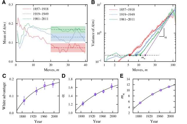
Next, we considered the time evolution of the variance for matches ending in draws (Fig. 3B). Surprisingly, $\alpha$ seems to be approaching a value close to that for a ballistic regime. We found that the exponent $\alpha$ follows an exponential approach with a characteristic time of $128\pm 9$ years to the asymptote $\alpha=1.9\pm 0.1$ (Fig. 3D). We surmise that this trend is directly connected to an increase in the typical difference in fitness among players. Specifically, the presence of fitness in a diffusive process has been shown to give rise to ballistic diffusion Skalski . For an illustration of how differences in fitness are related to a ballistic regime ($\alpha=2$), assume that

$$A_{i}(m+0.5)=A_{i}(m)+\Phi_{i}+\eta(m)$$ (1)

describes the advantage of the white player in a match $i$, where the difference in fitness between two players is $\Phi_{i}$ and $\eta(m)$ is a Gaussian variable. $\Phi_{i}>0$ yields a positive drift in $A_{i}(m)$ thus modeling a match where the white player is better. Assuming that the fitness $\Phi_{i}$ is drawn from a distribution with finite variance $\sigma^{2}_{\Phi}$, it follows that

$$\sigma^{2}(m)\sim\sigma^{2}_{\Phi}\,m^{2}\,.$$ (2)

Thus, $\alpha=2$. In the case of chess, the diffusive scenario is not determined purely by the fitness of players. However, differences in fitness are certainly an essential ingredient and thus Eq.(1) can provide insight into the data of Fig. 3D by suggesting that the typical difference in skill between players has been increasing.

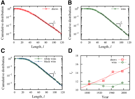
A striking feature of the results of Fig. 3B is the drift of the crossover move $m_{\times}$ at which the power-law regime begins. We observe that $m_{\times}$ is exponentially approaching an asymptote at $15.6\pm 0.6$ moves with a characteristic time of $130\pm 12$ years (Fig. 3E). Based on the existence of limiting values for $\alpha$ and $m_{\times}$, we plot in Figure 3B an extrapolated power law to represent the limiting diffusive regime (continuous line). We have also found that the distributions of the match lengths for wins and draws display exponential decays with characteristics lengths of $13.22\pm 0.02$ moves for draws and $11.20\pm 0.02$ moves for wins. Moreover, we find that these characteristic lengths have changed over the history of chess. For matches ending in draws, we observed a statistically significant growth of approximately $3.0\pm 0.7$ moves per century. For wins, we find no statistical evidence of growth and the characteristic length can be approximated by a constant mean of $11.3\pm 0.6$ moves (supplementary Fig. 1).

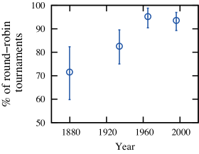
A question posed by the time evolution of these quantities is whether the observed changes are due to learning by chess players over time or due to a secondary factor such as changes in the organization of chess tournaments. In order to determine the answer to this question, we analyze the type of tournaments included in the database. We find that 88$\%$ of the tournaments in the database use “round-robin” pairing (all-play-all) and that there has been an increasing tendency to employ this pairing scheme (supplementary Fig. 2). In order to further strengthen our conclusions, we analyze the matches in the database obtained by excluding tournaments that do not use round-robin pairing. This procedure has the advantage that it reduces the effect of non-randomness sampling. As shown in supplementary Fig. 3, this procedure does not change the results of our analyses.

We next studied the distribution profile of the advantage. We use the normalized advantage

$$\xi(m)=\frac{A(m)-\langle A(m)\rangle}{\sigma(m)}\,,$$ (3)

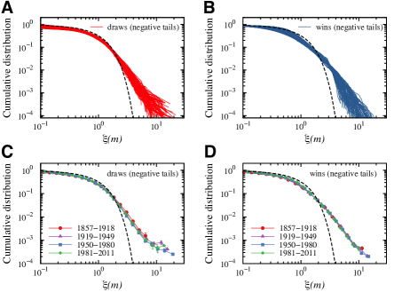
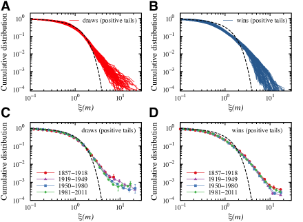
where $\langle A(m)\rangle$ is the mean value of advantage after $m$ moves and $\sigma(m)$ is the standard-deviation. Figures 4A and 4B show the positive tails of the cumulative distribution of $\xi(m)$ for draws and wins for $10\leq m\leq 70$. We observe the good data collapse, which indicates that the advantages are statistically self-similar, since after scaling they follow the same universal distribution. Moreover, Figs. 4D and 4E show that the distribution profile of the normalized advantage is quite stable over the last 150 years. These distributions obey a functional form that is significantly different from a Gaussian distribution (dashed line in the previous plots). In particular, we observe a more slowly decaying tail, showing the existence of large fluctuations even for matches ending in draws.

Figure 4: Scale invariance and non-Gaussian properties of the white player’s advantage. Positive tails of the cumulative distribution function for the normalized advantage $\xi(m)$ for matches ending in (A) draws and (B) wins. Each line in these plots represents a distribution for a different value of $m$ in the range 10 to 70. By match outcome, the distributions for different values of $m$ exhibit a good data collapse with tails that decay slower than a Gaussian distribution (dashed line). Average cumulative distribution for matches ending in (C) draws and (D) wins for four time periods. We estimated the error bars using bootstrapping. These data support the hypothesis of scaling, that is, the distributions follow a universal non-Gaussian functional form. The negative tails present a very similar shape (see supplementary Fig. 4).

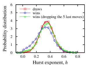
Another intriguing question is whether there is memory in the evolution of the white player’s advantage. To investigate this hypothesis, we consider the time series of advantage increments $\Delta A(m)=A(m+0.5)-A(m)$ for all 5,154 matches ending in a draw that are longer than $50$ moves. We used detrended fluctuation analysis (DFA, see Methods Section B) to obtain the Hurst exponent for each match (Fig. 5A). We find $h$ distributed around $0.35$ (Fig. 5B) which indicates the presence of long-range anti-correlations in the evolution of $A(m)$. A value of $h<0.5$ indicates the presence of an anti-persistent behavior, that is, the alternation between large and small values of $\Delta A(m)$ occurs much more frequently than by chance. This result also agrees with the oscillating behavior of the mean advantage (Fig. 1B). We also find that the Hurst exponent $h$ has evolved over time (Fig. 5C). In particular, we note that the anti-persistent behavior has statistically increased for the recent two periods, indicating that the alternating behavior has intensified in this period. We have found a very similar behavior for matches ending in wins after removing the last few moves in the match (supplementary Fig. 5).

Figure 5: Long-range correlations in white player’s advantage. (A) Detrended fluctuation analysis (DFA, see Methods Section B) of white player’s advantage increments, that is, $\Delta A(m)=A(m+0.5)-A(m)$, for a match ended in a draw and selected at random from the database. For series with long-range correlations, the relationship between the fluctuation function $F(s)$ and the scale $s$ is a power-law where the exponent is the Hurst exponent $h$. Thus, in this log-log plot the relationship is approximated by a straight line with slope equal to $h=0.345$. In general, we find all these relationships to be well approximated by straight lines with an average Pearson correlation coefficient of $0.892\pm 0.002$. (B) Distribution of the estimated Hurst exponent $h$ obtained using DFA for matches longer than 50 moves that ended in a draw (squares). The continuous line is a Gaussian fit to the distribution with mean $0.35$ and standard-deviation $0.1$. Since $h<0.5$, it implies an anti-persistent behavior (see Fig. 1B). We have also evaluated the distribution of $h$ using the shuffled version of these series (circles). For this case, the dashed line is a Gaussian fit to the data with mean $0.54$ and standard-deviation $0.09$. Note that the shuffled procedure removed the correlations, confirming the existence of long-range correlations in $A(m)$. (C) Historical changes in the mean Hurst exponent $h$. Note the significantly small values of $h$ in recent periods, showing that the anti-persistent behavior has increased for more recent matches.

Discussion

We have characterized the advantage dynamics of chess matches as a self-similar, super-diffusive and long-ranged-memory process. Our investigation provides insights into the complex process of creating and disseminating knowledge of a complex system at the population-level. By studying 150 years of high level chess, we presented evidence that the dynamics of a chess have evolved over time in such a way that it appears to be approaching a steady-state. The baseline advantage of the white player, the cross-over move $m_{\times}$, and the diffusive exponent $\alpha$ are exponentially approaching asymptotes with different characteristic times. We hypothesized that the evolution of $\alpha$ are closely related to an increase in the difference of fitness among players, while the evolution of the baseline advantage of white player indicates that players are learning better ways to explore this advantage. The increase in the cross-over move $m_{\times}$ suggest that the opening stage of a match is becoming longer which may also be related to a collective learning process. As discussed earlier, hypothesized historical changes in pairing scheme during tournaments cannot explain these findings.

Methods

Estimating $A(m)$

The core of a chess program is called the chess engine. The chess engine is responsible for finding the best moves given a particular arrangement of pieces on the board. In order to find the best moves, the chess engine enumerates and evaluates a huge number of possible sequences of moves. The evaluation of these possible moves is made by optimizing a function that usually defines the white player’s advantage. The way that the function is defined varies from engine to engine, but some key aspects, such as the difference of pondered number of pieces, are always present. Other theoretical aspects of chess such as mobility, king safety, and center control are also typically considered in a heuristic manner. A simple example is the definition used for the GNU Chess program in 1987 (see http://alumni.imsa.edu/$\sim$stendahl/comp/txt/gnuchess.txt). There are tournaments between these programs aiming to compare the strength of different engines. The results we present were all obtained using the Crafty™  engine Crafty . This is a free program that is ranked 24th in the Computer Chess Rating Lists (CCRL - http://www.computerchess.org.uk/ccrl). We have also compared the results of subsets of our database with other engines, and the estimate of the white player advantage proved robust against those changes.

DFA

DFA consists of four steps Peng ; Kantelhardt :

1. We define the profile

   $$Y(i)=\sum_{k=1}^{i}\Delta A(m)-\langle\Delta A(m)\rangle\,;$$

2. We cut $Y(i)$ into $N_{s}=N/s$ non-overlapping segments of size $s$, where $N$ is the length of the series;

3. For each segment a local polynomial trend (here, we have used linear function) is calculated and subtracted from $Y(i)$, defining $Y_{s}(i)=Y(i)-p_{\nu}(i)$, where $p_{\nu}(i)$ represents the local trend in the $\nu$-th segment;

4. We evaluate the fluctuation function

   $$F(s)=[\frac{1}{N_{s}}\sum_{\nu=1}^{N_{s}}\langle Y_{s}(i)^{2}\rangle_{\nu}]^{1/2}\,,$$

   where $\langle Y_{s}(i)^{2}\rangle_{\nu}$ is mean square value of $Y_{s}(i)$ over the data in the $\nu$-th segment.

If $A(m)$ is self-similar, the fluctuation function $F(s)$ displays a power-law dependence on the time scale $s$, that is, $F(s)\sim s^{h}$ , where $h$ is the Hurst exponent.

Supporting information

Table S1: Full description of our chess database. This table show all the tournaments that comprise our data base. The PGN files are free available at http://www.pgnmentor.com/files.html. Specifically, the files we have used are those grouped under sections “Tournaments”, “Candidates and Interzonals” and “World Championships”.

Tournament	Years
World Championships
FIDE Championship	1996,1998-2000,2002,2004-2008,2010
PCA Championship	1993,1995
World Championship	1886,1889,1890,1892,1894,1896,1907-1910,1921,1927,1929,1934,1935,
	1937,1948,1951,1954,1957,1958,1960,1961,1963,1966,1969,1972,1978,
	1981,1985,1987,1990,1993
Candidates and Interzonals
Candidates	1950,1953,1959,1962,1965,1968,1971,1974,1980,1983,1985,1990,1994
Interzonals	1948,1952,1955,1958,1962,1964,1967,1970,1973,1976,1979,1982,1985,
	1987,1990,1993
WCC Qualifier	1998,2002,2007,2009
PCA Candidates	1994
PCA Qualifier	1993
World Cup	2005
Open Tournaments
AVRO	1938
Aachen	1868
Altona	1869,1872
Amsterdam	1889,1920,1936,1976-1981,1985,1987,1988,1991,1993-1996
Bad	1977
BadElster	1937-1939
BadHarzburg	1938,1939
BadKissingen	1928,1980,1981
BadNauheim	1935-1937
BadNiendorf	1927
BadOeynhausen	1922
BadPistyan	1912,1922
Baden	1870,1925,1980
Barcelona	1929,1935,1989
Barmen	1869,1905
Belfort	1988
Belgrade	1964,1993,1997
Berlin	1881,1897,1907,1920,1926
Bermuda	2005
Bern	1932
Beverwijk	1967
Biel	1992,1997,2004,2006,2007
Bilbao	2009
Birmingham	1858
Bled	1931,1961,1979
Bournemouth	1939
Bradford	1888,1889
Breslau	1889,1912,1925
Bristol	1861
Brussels	1986-1988
Bucharest	1953
Budapest	1896,1913,1921,1926,1929,1940,1952,2003
Budva	1967
Buenos Aires	1939,1944,1960,1970,1980,1994
Bugojno	1978,1980,1982,1984,1986
Cambridge	1904
Cannes	2002
Carlsbad	1907
Carrasco	1921,1938
Chicago	1874,1982
Cleveland	1871
Coburg	1904
Cologne	1877,1898
Copenhagen	1907,1916,1924,1934
Dallas	1957
Debrecen	1925
Dortmund	1928,1973,1975-1989,1991-2007
DosHermanas	1991-1997,1999,2001,2003,2005
Dresden	1892,1926
Duisburg	1929
Dundee	1867
Dusseldorf	1862,1908
Enghien	2003
Foros	2007
Frankfurt	1878,1887,1923,1930
Geneva	1977
Giessen	1928
Gijon	1944,1945
Gothenburg	1909,1920
Groningen	1946
Hague	1928
Hamburg	1885,1910,1921
Hannover	1902
Hastings	1895,1919,1922,1923,1925-1927,1929-1938,1945,1946,1949,1950,1953,
	1954,1957,1959-1962,1964,1966,1969-2004
Havana	1913,1962,1963,1965
Heidelberg	1949
Hilversum	1973
Hollywood	1945
Homburg	1927
Hoogeveen	2003
Johannesburg	1979,1981
Karlovy	1948
Karlsbad	1911,1923,1929
Kecskemet	1927
Kemeri	1937,1939
Kiel	1893
Kiev	1903
Krakow	1940
Kuibyshev	1942
LakeHopatcong	1926
LasPalmas	1973-1978,1980-1982,1991,1993,1994,1996
Leiden	1970
Leipzig	1876,1877,1879,1894
Leningrad	1934,1937,1939
Leon	1996
Liege	1930
Linares	1981,1983,1985,1988-1995,1997-2007
Ljubljana	1938
Ljubojevic	1975,1977
Lodz	1907,1935,1938
London	1862,1866,1872,1876,1877,1883,1892,1900,1922,1927,1932,1946,1980,
	1982,1984,1986
LosAngeles	1963
Lugano	1970
Lviv	2000
Madrid	1943,1996,1997,1998
Maehrisch	1923
Magdeburg	1927
Manchester	1857,1890
Manila	1974, 1975
Mannheim	1914
MardelPlata	1928,1934,1936,1942-1957,1959-1962,1965-1972,1976,1979,1981,1982
Margate	1935,1939
Marienbad	1925
Meran	1924
Merano	1926
Merida	2000,2001
Milan	1975
MonteCarlo	1901-1904,1967
Montecatini	2000
Montevideo	1941
Montreal	1979
Moscow	1899,1901,1920,1925,1935,1947,1956,1966,1967,1971,1975,1981,1985,
	1992,2005-2007
Munich	1900,1941,1942,1993
Netanya	1968,1973
NewYork	1857,1880,1889,1893,1894,1913,1915,1916,1918,1924,1927,1931,1940,
	1951
Nice	1930
Niksic	1978,1983
Noordwijk	1938
Nottingham	1936
Novgorod	1994-1997
NoviSad	1984
Nuremberg	1883,1896,1906
Oslo	1984
Ostende	1905-1907,1937
Palma	1967,1968,1970,1971
Paris	1867,1878,1900,1924,1925,1933
Parnu	1937,1947,1996
Pasadena	1932
Philadelphia	1876
Podebrady	1936
Poikovsky	2004-2007
Polanica	1998,2000
Portoroz	1985
Prague	1908,1943
Ramsgate	1929
ReggioEmilia	1985-1989,1991,1992
Reykjavik	1987,1988,1991
Riga	1995
Rogaska	1929
Rosario	1939
Rotterdam	1989
Rovinj	1970
Salzburg	1943
SanAntonio	1972
SanRemo	1930
SanSebastian	1911,1912
SantaMonica	1966
Sarajevo	1984,1999,2000
Scarborough	1930
Semmering	1926
Skelleftea	1989
Skopje	1967
Sliac	1932
Sochi	1973,1982
Sofia	2005,2007
SovietChamp	1920,1923-1925,1927,1929,1931,1933,1934,1937,1939,1940,1944,
	1945,1947-1953,1955-1981,1983-1991
StLouis	1904
StPetersburg	1878,1895,1905,1909,1913
Stepanakert	2005
Stockholm	1930
Stuttgart	1939
Sverdlovsk	1943
Swinemunde	1930,1931
Szcawno	1950
Teeside	1975
Teplitz	1922
TerApel	1997
Tilburg	1977-1989,1991-1994,1996-1998
Titograd	1984
Trencianske	1941,1949
Triberg	1915,1921
Turin	1982
Ujpest	1934
Vienna	1873,1882,1898,1899,1903,1907,1908,1922,1923,1937,1996
Vilnius	1909,1912
Vinkovci	1968
Vrbas	1980
Waddinxveen	1979
Warsaw	1947
WijkaanZee	1968-2007
Winnipeg	1967
Zagreb	1965
Zandvoort	1936

Figure S1: Historical trends in match lengths. Cumulative distribution function for the match lengths ending in (A) draws and wins (B). Both distributions display an exponential decay with characteristic lengths $13.22\pm 0.02$ for draws and $11.20\pm 0.02$ for wins. (C) Cumulative distribution function for the match lengths ending white wins (circles) and black wins (triangles). Note that both distributions are almost indistinguishable. (D) Changes in the characteristic game length $l_{c}$ over time. For draws (squares), we observe a statistically significant growth of approximately $3.0\pm 0.7$ moves per century (red line). For wins (circles), we find that $l_{c}$ is approximately constant with mean value $11.3\pm 0.6$ (green line).

Figure S2: Percentage of tournaments that employ the round-robin (all-play-all) pairing scheme. Note the increase in the fraction of tournaments employing round-robin pairing scheme.

Figure S3: The effect of excluding tournaments using the swiss-pairing scheme on the historical trends reported in Fig. 3. It is visually apparent that excluding data from those tournaments does not significantly change our results. Thus, temporal changes in the pairing schemes used in chess tournaments can not explain our findings.

Figure S4: Scale invariance and non-Gaussian properties of the white player’s advantage. Negative tails of the cumulative distribution function for the normalized advantage $\xi(m)=\frac{A(m)-\langle A(m)\rangle}{\sigma(m)}$ for matches ending in (A) draws and (B) wins. Each line in these plots represents a distribution for a different value of $m$ in the range 10 to 70. For match outcome, the distributions for different values of $m$ exhibit a good data collapse with tails that decay slower than a Gaussian distribution (dashed line). Average cumulative distribution for matches ending in (C) draws and (D) wins for four time periods. We estimated the error bars using bootstrapping.

Figure S5: Match outcome and long-range correlations in the white player’s advantage. Distribution of the estimated Hurst exponent $h$ obtained using DFA for matches longer than 50 moves that ended in draws (squares), wins (circles) and wins after dropping the five last moves of each match. The continuous line is a Gaussian fit to the distribution for draws with mean $0.35$ and standard-deviation $0.10$. For wins, the mean value of $h$ is $0.31$ and the standard-deviation is $0.13$. Note that after dropping the five last moves the distribution of $h$ for wins becomes very close to distribution obtained for draws. The mean value in this last case is $0.35$ and the standard-deviation is $0.11$.

References

- (1) Amaral LAN, Ottino JM (2004) Augmenting the framework for the study of complex systems. Eur. Phys. J. B 38: 147-162.
- (2) Fortunato S, Castellano S (2007) Scaling and universality in proportional elections. Phys. Rev. Lett. 99: 138701.
- (3) Ratkiewicz J, Fortunato S, Flammini A, Menczer F, Vespignani A (2010) Characterizing and modeling the dynamics of online popularity. Phys. Rev. Lett. 105: 158701.
- (4) Rozenfeld HD, Rybski D, Andrade JS, Batty M, Stanley HE, Makse HA (2008) Laws of population growth. Proc. Natl. Acad. Sci. USA 105: 18702-18707.
- (5) Bialek W, Cavagna Q, Giardina I, Mora T, Silvestri E, Viale M, Walczak AM (2012) Statistical mechanics for natural flocks of birds. Proc. Natl. Acad. Sci. USA 109: 4786-4791.
- (6) Peruani F, Starruß J, Jakovljevic V, Søgaard-Andersen L, Deutsch A, Bär M (2012) Collective motion and nonequilibrium cluster formation in colonies of gliding bacteria. Phys. Rev. Lett. 108: 098102.
- (7) Stringer MJ, Sales-Pardo M, Amaral LAN (2008) Effectiveness of journal ranking schemes as a tool for locating information. PLoS ONE 3: e1683.
- (8) O’Brien C (1994) Checkmate for chess historians. Science 265: 1168-1169.
- (9) Shannon CE (1950) Programming a computer for playing chess. Philosophical Magazine 41: 314.
- (10) Blasius B, Tönjes R (2009) Zipf’s law in the popularity distribution of chess openings. Phys. Rev. Lett. 103: 218701.
- (11) Gobet F, de Voogt A, Retschitzki J (2004) Moves in Mind: The Psychology of Board Games. New York: Psychology Press.
- (12) Saariluoma P (1995) Chess Players’ Thinking: A Cognitive Psychological Approach. London: Routledge.
- (13) Fogel DB, Hays TJ, Hahn SL, Quon J (2004) A self-learning evolutionary chess program. Proceedings of the IEEE 92: 1947-1954.
- (14) Elo A (1978) The Rating of Chess Players, Past and Present. London: Batsford.
- (15) Hyatt RM, Crafty Chess v23.3, www.craftychess.com (accessed on July 2011).
- (16) Siegle P, Goychuk I, Hänggi P (2010) Origin of hyperdiffusion in generalized brownian motion. Phys. Rev. Lett. 105: 100602.
- (17) Skalski GT, Gilliam JF (2000) Modeling diffusive spread in a heterogeneous population: a movement study with stream fish. Ecology 81: 1685-1700.
- (18) Peng CK, Buldyrev SV, Havlin S, Simons M, Stanley HE, Goldberger AL (1994) Mosaic organization of DNA nucleotides. Phys Rev E 49: 1685-1689.
- (19) Kantelhardt JW, Koscielny-Bunde E, Rego HHA, Havlin S, Bunde A (2001) Detecting long-range correlations with detrended fluctuation analysis. Physica A 295: 441-454.